Abstract

We offer the parameter, interpreted as the ”chemical potential”, which is sensitive to the first order phase transition: it must decrease with number of evaporating (produced) particles (hadrons) if the (interacting hadron or/and QCD plasma) medium is boiling and it increase if no phase transition occur. The main part of the paper is devoted to the question: how one can measure the ”chemical potential” in the hadron inelastic processes. Our definition of this parameter is quite general but assumes that the hadron multiplicity is sufficiently large. The simple transparent phenomenological lattice gas model is considered for sake of clarity only.

1 Introduction

Despite the fact that the first order phase transition in the ion collisions is widely discussed both from theoretical [1] and experimental [2] points of view the feeling of some dissatisfaction nevertheless remain. To all appearance the main problem consists in absence of the single-meaning directly measurable (”order”) parameter(s) which may confirm this phenomenon in the high energy experiment. Our aim is to offer such parameter, explain its physical meaning and to show how it can be measured.

We guess that to observe first order phase transition it is necessary to consider very high multiplicity (VHM) processes. Then in this multiplicity region exist following parameter:

$$\mu(n,s)\simeq-\frac{T(n,s)}{n}\ln\sigma_{n}(s),$$ (1. 1)

Here $\sigma_{n}$ is the normalized to unite multiplicity distribution which can be considered in the VHM region as the ”partition function” of the $equilibrium$ system, see Appendix, and $T$ is the mean energy of produced particles, i.e. $T$ is associated with temperature. Continuing the analogy with thermodynamics one can say that $(-T\ln\sigma_{n})/n$ is the Gibbs free energy per one particle. Then $\mu$ can be interpreted as the ”chemical potential” measured with help of $observed$ particles in a free state.

We assume that the system obey the equilibrium condition, i.e. produced particles energy distribution can be described with high accuracy by Boltzmann exponent, or, it is the same, the inequality (b̊) must be satisfied. This assumption defines the ”VHM region” [3] . It must be underlined that existence of the ”good” parameter $T$ does not assumes that the whole system is thermally equilibrium, i.e. the energy spectrum of unobserved particles may be arbitrary in our ”inclusive” description.

The definition (1̊.1) is quiet general. It can be used both for hadron-hadron and ion-ion collisions, both for low and high energies. It is model free and operates only with ”external” directly measurable parameters. The single indispensable condition: we work in the $VHM$ region of observed particles. It is evident that such generality has definite defect: measuring $\mu$ one can not say something about details of the process.

This ”defect” have following explanation. The point is that the classical theory of phase transitions have dealing immediately with the $internal$ properties of media in which the transition occur. But in our, ”$S$-matrix”, case one can examine only the $external$ response on the phase transition in the form of created mass-shell particles.

Continuing the analogy with the boiling, we are trying to define the boiling by the number of evaporating particles. The effect is evidently seen if the number of such particles is very large, i.e. in the VHM case. The ”order parameter” is the work needed for one particle production, i.e. coincides with the ”chemical potential”. In the boiled ”two-phase” region the media is unstable against ”evaporation” of particles, i.e. the chemical potential must decrease with number of produced particles.

We offer quantitative answers on the following three question.

(A) In what case one may observe first order phase transition.
We will argue that observation of VHM states are necessary to find phase transition phenomenon. First of all the energy of produced particles are small in VHM case. This means that the kinetic degrees of freedom does not play essential role, i.e. they can not destroy, wipe out, the phase transition phenomenon. The second reason is connected with observation that in the VHM region one may use such equilibrium thermodynamics parameters as the temperature $T(n,s)$, chemical potential $\mu(n,s)$ and so on.

(B) What we can measure.
We will see that in VHM region exist the estimation (1̊.1) where all quantities in r.h.s. are measurables.

(C) What kind effect one may expect.
Chemical potential, $\mu(n,s)$, by definition is the work which is necessary to introduce, i.e. to produce, one particle into the system [4] . If the first order pase transition occurs then $\mu(n,s)$ must decrease with $n$ in the two-phase (”boiling”) region. It is our general conclusion which will be explained using lattice gas model.

2 Definitions

2.1

We will start from simple generalization of well known formulae. Let us consider the generating function

$$\rho(z,s)=\sum_{n=0}^{\infty}z^{n}\sigma_{n}(s).$$ (2. 2)

For sake of simplicity $\sigma_{n}$ is normalized so that

$$\rho(1,s)=1.$$ (2. 3)

One may use inverse Mellin transformation:

$$\sigma_{n}(s)=\frac{1}{2\pi i}\oint\frac{dz}{z^{n+1}}\rho(z,s)$$ (2. 4)

to find $\sigma_{n}$ if $\rho(z,s)$ is known. Noting that $\sigma_{n}$ have sharp maximum over $n$ near mean multiplicity $\bar{n}(s)$ one may calculate integral (m̊el) by saddle point method. The equation:

$$n=\frac{\partial}{\partial\ln z}\ln\rho(z,s)$$ (2. 5)

defines mostly essential value $z=z(n,s)$. Notice that $\sigma_{n}\equiv 0$ if the hadron multiplicity $n>n_{max}=\sqrt{s}/m$, where $m$ is the characteristic mass of hadron. Production of identical particles is considered for sake of simplicity. Therefore, only $z<z_{max}=z(n_{max},s)$ have the physical meaning.

One may write $\rho(z,s)$ in the form:

$$\rho(z,s)=\exp\left\{\sum_{l=0}^{\infty}z^{l}b_{l}(s)\right\},$$ (2. 6)

where the Mayer group coefficient $b_{l}$ can be expressed through $k$-particle correlation function (binomial moments) $c_{k}(s)$:

$$b_{l}(s)=\sum_{k=l}^{\infty}\frac{(-1)^{(k-l)}}{l!(k-l)!}c_{k}(s).$$ (2. 7)

Let us assume now that in the sum:

$$\ln\rho_{(}z,s)=\sum_{k}\frac{(z-1)^{k}}{k!}c_{k}(s)$$ (2. 8)

one may leave first term. Then it is easy to see that

$$z(n,s)=n/c_{1}(s),~{}c_{1}(s)\equiv\bar{n}(s),$$ (2. 9)

are essential and in the VHM region

$$\ln\sigma_{n}(s)=-n\ln\frac{n}{c_{1}(s)}(1+O(1/\ln n))=-n\ln z(n,s)(1+O(1/\ln n)).$$ (2. 10)

Therefore, in considered case with $c_{k}=0,~{}k>1,$ exist following asymptotic estimation for $n>>1$:

$$\ln\sigma_{n}\simeq-n\ln z(n,s),$$ (2. 11)

i.e. $\sigma_{n}$ is defined in VHM region mainly by the solution of Eq.(e̊q1) and the correction can not change this conclusion. It will be shown that this kind of estimation is hold for arbitrary asymptotics of $\sigma_{n}$.

If we understand $\sigma_{n}$ as the ”partition function” in the VHM region then $z$ is the $activity$ usually introduced in statistical physics if the number of particles is not conserved. Correspondingly the chemical potential $\mu$ is defined trough $z$:

$$\mu=T\ln z.$$ (2. 12)

Combining this definition with estimation (1̊.10) we define $\sigma_{n}$ through $\mu$. But, if this estimation does not depend from the asymptotics of $\sigma_{n}$, it can be used for definition of $\mu(n,s)$ through $\sigma_{n}(s)$ and $T(n,s)$. Just this idea is realized in (1̊.1).

2.2

Now we will make the important step. To put in a good order our intuition it is useful to consider $\rho(z,s)$ as the $nontrivial$ function of $z$. In statistical physics the thermodynamical limit is considered for this purpose. In our case the finiteness of energy $\sqrt{s}$ and of the hadron mass $m$ put obstacles on this way since the system of produced particles necessarily belongs to the energy-momentum surface. But we can continue theoretically $\sigma_{n}$ to the range $n>n_{max}$ and consider $\rho(z,s)$ as the nontrivial function of $z$.

Let us consider the analog generating function which has the first $n<n_{max}$ coefficient of expansion over $z$ equal to $\sigma_{n}$ and higher coefficients for $n\geq n_{max}$ are deduced from continuation of theoretical value of $\sigma_{n}$ to $n\geq n_{max}$. Then the inverse Mellin transformation (m̊el) gives a good estimation of $\sigma_{n}$ through this generating function if the fluctuations near $z(n,s)$ are Gaussian or, it is the same, if

$$\left.\frac{|2n-z^{3}\partial^{3}\ln\rho(z,s)/\partial z^{3}|}{|n+z^{2}\partial^{2}\ln\rho(z,s)/\partial z^{2}|^{3/2}}\right|_{z=z(n,s)}<<1.$$ (2. 13)

Notice that if the estimation (1̊.10) is generally rightful then one can easily find that l.h.s. of (z̊) is $\sim 1/n^{1/2}$. Therefore, one may consider $\rho(z,s)$ as the nontrivial function of $z$ considering $z(n,s)<z_{max}$ if $n_{max}>>n>>1$.

Then it is easily deduce that the asymptotics of $\sigma_{n}(s)$ is defined by the leftmost singularity, $z_{c}$, of in this way generalized function $\rho(z,s)$ since, as it follows from (e̊q1), the singularity ”attracts” the solution $z(n,s)$ in the VHM region. In result, we may classify asymptotics of $\sigma_{n}$ in the VHM region if (z̊) is hold.

Thus our problem is reduced to the definition of possible location of leftmost singularity of $\rho(z,s)$ over $z>0$. It must be stressed that the character of singularity is not important for definition of $\mu(n,s)$ in the VHM region at least with $O(1/\ln n)$ accuracy. One may consider only three possibility: at $n\to\infty$

(A) $z(n,s)\to z_{c}=1$,

(B) $z(n,s)\to z_{c},~{}~{}1<z_{c}<\infty$,

(C) $z(n,s)\to z_{c}=\infty$.

Other possibilities are nonphysical or extremely rear. Correspondingly one may consider only three type of asymptotics in the VHM region:

(A) $\sigma_{n}>O(e^{-n})$. We will see that in this case the isotropic momentum distribution must be observed, i.e. the energy, $\varepsilon$, distribution in this case is Boltzmann-like, $\sim e^{-\beta\epsilon}$;

(B) $\sigma_{n}=O(e^{-n})$. Such asymptotics is typical for hard processes with large transverse momenta, like for jets [5] ;

(C) $\sigma_{n}<O(e^{-n})$. This asymptotic behavior is typical for multiperipheral-like kinematics, where the longitudinal momenta of produced particles are noticeably higher than the transverse ones [6] .

We are forced to assume that the energy is sufficiently large, i.e. $z_{max}$ is sufficiently close to $z_{c}$. In opposite case the singularity would not be ”seen” on experiment.

Our aim is to give physical interpretation of this three asymptotics. The idea, as it follows from previous discussion, is simple: one must explain the nature of singularity $z_{c}$. It must be noted at the same time that in the equilibrium thermodynamics exist only two possibility, (A) and (C) [13] and just the case (A) corresponds to the first order phase transition.

Summarizing the results we conclude: if the energy is sufficiently large, i.e. if $z_{max}$ is sufficiently close to $z_{c}$, if the multiplicity is sufficiently large, so that (b̊) is satisfied and $z(n,s)$ can be sufficiently close to $z_{c}$, then one may have confident answer on the question: exist or not first order phase transition in hadron collisions.

It must be noted here that the heavy ion collisions are the most candidates since $z_{c}$ is easer distinguishable in this case.

2.3

The temperature $T$ is the another problem. The temperature is introduced usually using Kubo-Martin-Schwinger (KMS) periodic boundary conditions [7] . But this way assumes from the very beginning that the system (a) is equilibrium [8] and (b) is surrounded by thermostat through which the temperature is determined. The first condition (a) we take as the simplification which gives the equilibrium state where the time ordering in the particle production process is not important and therefore the time may be excluded from consideration.

The second one (b) is the problem since there is no thermostat in particle physics. For this reason we introduce the temperature as the Lagrange multiplier $\beta=1/T$ of energy conservation law [3] . In such approach the condition that the system is in equilibrium with thermostat replaced by the condition that the fluctuations in vicinity of $\beta$ are Gaussian.

The interesting for us $\rho(z,{s})$ we define through inverse Laplace transform of $\rho(z,\beta)$:

$$\rho(z,s)=\int\frac{d\beta}{2\pi i\sqrt{s}}e^{\beta\sqrt{s}}\rho(z,\beta).$$ (2. 14)

It is known [8] that if the interaction radii is finite then the equation (of state):

$$\sqrt{s}=-\frac{\partial}{\partial\beta}\rho(z,\beta)$$ (2. 15)

have real positive solution $\beta(n,s)$ at $z=z(n,s)$. We will assume that the fluctuations near $\beta(n,{s})$ are Gaussian. This means that the inequality [3] :

$$\left.\frac{|\partial^{3}\ln\rho(z,\beta)/\partial\beta^{3}|}{|\partial^{2}\ln\rho(z,\beta)/\partial\beta^{2}|^{3/2}}\right|_{z=z(n,s),\beta=\beta(n,s)}<<1$$ (2. 16)

is satisfied. Therefore, we prepare the formalism to find thermodynamic description of the processes of particle production assuming that this $S$-matrix conditions of equilibrium (z̊) and (b̊) are hold.

We want to underline that our thermal equilibrium condition (b̊) have absolute meaning: if it is not satisfied then $\beta(n,s)$ loses every sense since the expansion in vicinity of $\beta(n,s)$ leads to the asymptotic series. In this case only the dynamical description of $S$-matrix can be used.

It is not hard to see [3] that

$$\frac{\partial^{l}}{\partial\beta^{l}}\ln R(z,\beta)|_{z=z(n,s),\beta=\beta(n,s)}=<\prod_{i=1}^{l}(\epsilon_{i}-<\epsilon>)>_{n,s}$$ (2. 17)

is the $l$-point energy correlator, where $<...>_{n,s}$ means averaging over all events with given multiplicity and energy. Therefore (b̊) means ”relaxation of $l$-point correlations”, $l>2$, measured in units of the dispersion of energy fluctuations, $l=2$. One can note here the difference of our definition of thermal equilibrium from thermodynamical one [9] .

2.4

Let us consider now the estimation (1̊.1). It follows from (m̊el) that, up to the preexponential factor,

$$\ln\sigma(n,s)\approx-n\ln z(n,s)+\ln\rho(z(n,s),s).$$ (2. 18)

We want to show that, in a vide range of n from VHM area,

$$n\ln z(n,s)\gtrsim\ln\rho(z(n,s),s).$$ (2. 19)

Let as consider now the mostly characteristic examples.

(A) Singularity at $z=1$.
This case will be considered in Sec.3. In the used lattice gas approximation $\ln{z}(n)\sim n^{-5}$ and

$$\ln\sigma_{n}\approx n^{-4}=n\ln z(n)(1+O(1/n)).$$ (2. 20)

(B) Singularity at $z=1+1/\bar{n}_{j}(s)<\infty$:
$\ln\rho(z,s)=-\gamma\ln(1-\bar{n}_{j}(s)(z-1))$. In this case $z(n)=1+1/\bar{n}_{j}(s)-1/n\bar{n}_{j}(s)$ and

$$\ln\sigma_{n}\approx-n/\bar{n}_{j}(s)+\gamma\ln n=$$

$$=-n/\bar{n}_{j}(s)(1+O(\ln n/n)).$$ (2. 21)

(C) Singularity at $z=\infty$: $\ln\rho(z,s)=c_{k}(s)(z-1)^{k},~{}k\geq 1$.
In this case $z(n)=(n/kc_{k})^{1/k}>>1$ and

$$\ln\sigma_{n}\approx-n\ln z(n)(1+O(1/\ln n)).$$ (2. 22)

One can conclude:

(i) The definition (1̊.1) in the VHM region is rightful since the correction falls down with $n$. On this stage we can give only the estimation of correction but (1̊.1) gives the correct $n$ dependence.

(ii) Activity $z(n,s)$ tends to $z_{c}$ from the right in the case (A) and from the left if we have the case(B) or (C).

(iii) The accuracy of estimation of the ”chemical potential” (1̊.1) increase from (C) to (A).

3 Ising model: phase transition

The physical meaning of singularity over $z$ [10] may be illustrated by following simple model. As was mentioned above the singularity at $z=1$ is interpreted as the first order phase transition. Therefore, let us assume [11] that $\beta$ is so large that interacting particles strike together into clusters (drops). Then the Mayer’s group coefficient for the cluster from $l$ particle is

$$b_{l}(\beta)\sim e^{-\beta\tau l^{(d-1)/d}},$$

where $\tau l^{(d-1)/d}$, $l>>1$, is the surface tension energy, $d$ is the dimension. Therefore, if $d>1$ the series over $l$ in (2̊.4) diverges at al $z>1$. At the same time, the sum (2̊.4) converge for $z<1$.

We consider following analog model to describe condensation phenomenon in the particle production processes. Let us cover the space around interaction point by the net assuming that if the particle hit the knot we have $(-1)$ and $(+1)$ in opposite case. This ”lattice gas” model [4] has a good description in terms of Ising model [12] . We may regulate number of down oriented ”spins”, i.e. the number of produced particles, by external magnetic field $\mathcal{H}$. Therefore the ”activity” $z=e^{-\beta\mathcal{H}}$, i.e. $-\mathcal{H}$ is the ”chemical potential” [13] .

Calculation of the partition function means summation over all spin configurations with constraint $\sigma^{2}=1$. Here the ergodic hypothesis is used. It allows to exclude the time from consideration.

To have the continuum model we may spread normally the $\delta$-function of this constraint [16] :

$$\delta(\sigma^{2}-1)\sim e^{-(1-\sigma^{2})^{2}/\Delta}.$$

Therefore, the grand partition function of the model in the continuum limit looks as follows [13, 17] :

$$\rho(\beta,z)=\int D\sigma e^{-S(\sigma,\mathcal{H})},$$ (3. 23)

where the action

$$S(\sigma,\mathcal{H})=\int d^{3}x\left\{\frac{1}{2}(\nabla\sigma)^{2}-\varepsilon\sigma^{2}+\alpha\sigma^{4}-\lambda\sigma\right\}.$$ (3. 24)

The structure of contributions in (2̊.6) essentially depends on the sign of constant $\varepsilon$, see Fig.1 where the case $\varepsilon>0$ is shown. Following notations was used:

$$\varepsilon\sim(1-\frac{\beta_{c}}{\beta}),~{}\alpha\sim\frac{\beta_{c}}{\beta}>0,~{}\lambda\sim(\beta\beta_{c})^{1/2}\mathcal{H},$$ (3. 25)

where $1/\beta_{c}$ is the phase transition temperature. Phase transition takes place if $\beta>\beta_{c}$ ($T<T_{C}$), i.e. we will consider in present section $\varepsilon>0$. In this case the mean spin $<\sigma>\neq 0$. We will assume that $\beta>>\beta_{c}$ since in this case the fluctuation around $<\sigma>$ are small and calculations in this case became simpler. Considered model describes decay of unstable vacuum [18] .

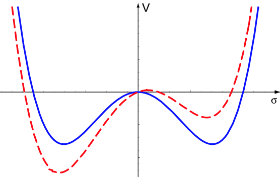
Figure 1: Solid line: undisturbed by $\mathcal{H}$ potential and dotted line includes $\mathcal{H}$.

The singularity over $\mathcal{H}$ appears by following reason. At $\mathcal{H}=0$ the potential

$$v=-\varepsilon\sigma^{2}+\alpha\sigma^{4}$$ (3. 26)

have two degenerate minima at $\sigma=\pm\sqrt{\varepsilon/2\alpha}$. The external field $\mathcal{H}<0$ we destroy this degeneracy. But in this case the system in the right-hand minimum (with the up-oriented spins) becomes unstable.

The branch point in the complex plane corresponds to this instability. The discontinuity gives [19] :

$$\rho(\beta,z)=\frac{a_{1}(\beta)}{\mathcal{H}^{4}}e^{-a_{2}(\beta)/\mathcal{H}^{2}},$$ (3. 27)

where ($\beta>\beta_{c}$)

$$a_{1}(\beta)=\frac{\pi^{2}}{2}\left(\frac{8\beta R^{4}}{9\beta_{c}A}\right)^{7/2}\left(\frac{1-\beta_{c}/\beta}{R^{2}}\right)^{3/4}\frac{R^{4}}{(\beta\beta_{c})^{2}},$$

$$a_{2}(\beta)=\frac{8\pi}{81\sqrt{2}}\frac{\beta}{\beta_{c}}\left(1-\frac{\beta_{c}}{\beta}\right)^{7/2}\frac{R^{4}}{(A\beta_{c}^{2})^{2}}.$$ (3. 28)

It must be noted that the eqs. (e̊q1) and (e̊q) have only one solution:

$$\beta(n,s)\to\beta_{c},~{}~{}\ln z(n,s)\equiv l(n,s)\to 0.$$

at increasing $n$. This means that the singularities at $T=T_{c}$ and $z=1$ attracts the solution:

$$l(n,\beta)\sim n^{-1/3}(\beta-\beta_{c})^{7/6},~{}~{}\beta(n,s)=\beta_{c}(1+\gamma/{n^{4}}),$$ (3. 29)

where $\gamma$ is the positive constant.

In result,

$$\ln\rho_{n}(s)\sim-n^{2/3}(1/n^{2/3})^{7}\sim-1/n^{4}~{}~{}~{}(\sim-n\ln z(n,s))$$ (3. 30)

decrees with $n$ and the chemical potential

$$\mu(n,s)\sim\frac{T_{c}}{n^{5}}(1+\gamma/n^{4})^{-1}$$ (3. 31)

also decrees with $n$.

Some comments will be useful to this Section:

1. One may note that $\sigma_{n}$ is defined by the discontinuity the the branch point in complex plane of $\ln z$ and decay of the meta-stable states does not play any role.

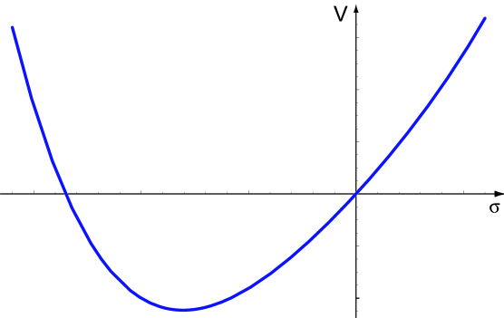
Figure 2: Stable ground state disturbed by $\mathcal{H}$.

2. It follows from (2̊.12) that, at fixed $\beta$,

$$\ln z_{c}\sim(1/n)^{1/3}<<1.$$ (3. 32)

This means that for large $n$ our calculations are correct. At the same time, in VHM region $z$ near unite is essential and it $decrees$ with $n$.

3. The work which is needed for production of one particle is $\sim\ln z(n,s)/\beta(n,s)$. Therefore production of large number of particles needs less work per one particle.

This conclusion have simple physical meaning (see beginning of present section). Let us consider decay of nonstable phase. The decay happens through production of clusters (domains with down oriented spins). The volume energy of cluster is $\propto R_{0}^{3}$, where $R_{0}$ is radius of cluster. It burst the dimension of cluster. If $R_{0}<R_{c}$, where $R_{c}$ is critical dimension of cluster, then the formation of such cluster is improbable. But if $R_{0}>R_{c}$ then the probability grows with radii of cluster. Latter explains why the chemical potential falls down with multiplicity.

4. In the VHM region the temperature, $T(n.s)$, tends to its critical value, $T_{c}$, and slowly depends on $n$.

4 Ising model: stable minimum

Let as consider the system with stable vacuum, $\beta<\beta_{c}$ ($T>T_{c}$) in (2̊.8). In this case, see Fig.2, the potential $v(\sigma)$ has unique minimum at $\sigma=0$. Switching on external field $\mathcal{H}$ the minimum move and the average spin appears, $\bar{\sigma}(\mathcal{H})\neq 0$. One can find it from the equation:

$$-\triangle\sigma+2\varepsilon\sigma+4\alpha\sigma^{3}=\lambda,~{}\varepsilon>0.$$

Having $\bar{\sigma}\neq 0$ we must expand the integral (2̊.6) near $\bar{\sigma}$:

$$\rho(\beta,z)=e^{\int dx\lambda\bar{\sigma}}e^{-W(\bar{\sigma})},$$ (4. 33)

where $W(\bar{\sigma})$ expandable over $\bar{\sigma}$:

$$W(\bar{\sigma})=\sum_{l=1}^{\infty}\frac{1}{l}\int\prod_{i=1}^{l}\{dx_{i}\bar{\sigma}(x_{i};\mathcal{H})\}B_{l}(x_{1},...,x_{l}),$$ (4. 34)

where $B_{l}$ is the $l$-point one particle irreducible vertex function. In another wards, $B_{l}$ play the role of virial coefficient. Comparing (3̊.2) with (2̊.4) one may consider $\bar{\sigma}$ as the affective activity of group of $l$ particles.

The representation (3̊.2) is useful since in the VHM region the density of particles is large and the particles momentum is small. Then, remembering that the virial decomposition is equivalent of decomposition over specific volume, calculating $B_{l}$ one may not go beyond the one-loop approximation, i.e. we may restricted by the semiclassical approximation.

Therefore, having large density one may neglect the spacial fluctuations. In this case the integral (2̊.6) is reduced down to the the usual Cauchy integral:

$$\rho(\beta,z)=\int_{-\infty}^{+\infty}d\sigma e^{-(\epsilon\sigma^{2}+\alpha\sigma^{4}+\lambda\sigma)}.$$ (4. 35)

In the VHM region $\lambda\sim\mathcal{H}\sim\ln z>>1$ is essential. It is easy to see that

$$\bar{\sigma}\simeq-(\lambda/4\alpha)^{1/3}$$ (4. 36)

is the extremum. The estimation of integral near this $\bar{\sigma}$ looks as follows:

$$\rho(\beta,z)\propto\left\{12\alpha\left(\frac{\lambda}{4\alpha}\right)^{2/3}\right\}^{-1/2}e^{3\lambda^{4/3}/4(4\alpha)^{1/3}}.$$ (4. 37)

This leads to increasing with $n$ activity:

$$l(n,s)\sim n^{8/3}$$ (4. 38)

and

$$\beta(n,s)\sim n^{2/3}.$$ (4. 39)

In result,

$$\ln\rho_{n}(s)\sim-n^{11/3}~{}(\sim-n\ln{z(n,s)}).$$ (4. 40)

A few comments at the end of this section:

(i) Cross section falls dawn in considered case faster then $O(e^{-n})$. The estimation:

$$\rho_{n}(s)\sim e^{-n\ln\bar{z}(n,s)}$$

gives the right expression in the VHM region.

(ii) The chemical potential increase with $n$:

$$\mu(n,s)=-(T(n,s)/n)\ln\sigma_{n}(s)\sim n^{2}.$$ (4. 41)

5 Conclusions

We may conclude that:

(i) We found definition of chemical potential (1̊.1). This important observable can be measured on the experiment directly where $T(n,s)$ is the mean energy of produced particles at given multiplicity $n$ and energy $\sqrt{s}$.

((ii) Being in the VHM region one may consider that $\mu(n,s)=O(1/n)$ at comparatively high multiplicities and it rise, $\mu(n,s)=O(n)$ with rising multiplicity, Fig.3, at comparatively low multiplicities. The transition region is defines the critical temperature $T_{c}$. But it is quiet possible that the condition (b̊) allows to see only one branch of the curve shown on Fig.3.

iv) The simplest example of finite $z_{c}$ presents the jet considered in the case (B), Fig.1. Hence case (C) has pure dynamical basis and can not be explained by equilibrium thermodynamics.

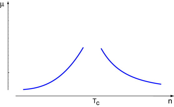
Figure 3: Chemical potential $\mu(n,s)$ as the function of multiplicity $n$. $T_{c}$ is the critical temperature. Breakthrough is the ”two-phase” region.

References

- [1] M. Creutz, Phys. Rev. D,15 1128 (1977); M. Gazdzicki and M. I. Gorenstein, Acta Physica Polonica B, 30 2705 (1999); A. N. Sissakian, A. S. Sorin, V. D. Toneev (Dubna, JINR) in Proceedings of 33rd International Conference on High Energy Physics (ICHEP 06), Moscow, Russia, 26 Jul - 2 Aug 2006 e-Print: nucl-th/0608032
- [2] BNL Report, Hunting the Quark Gluon Plasma, BNL-73847-2005; C. Alt et al. arXiv: nucl-ex/0710.0118
- [3] J. Manjavidze and A. Sissakian, Phys. Rep., 346 1 (2001).
- [4] A. Isikhara, Statistical physics, Mir, Moscow (1973).
- [5] I. C. Taylor, Phys.Lett. B, 73 85 (1978); A. J. MacFarlane and C. Woo, Nucl.Phys. B, 77 91 (1974).
- [6] E. Kuraev, L. Lipatov and V. Fadin, Sov. Phys. JETP, 44 443 (1976); Zh. Eksp. Teor. Fiz., 71 840 (1976); L. Lipatov, Sov. J. Nucl. Phys., 20 94 (1975); V. Gribov and L. Lipatov, Sov. J. Nucl. Phys., 15 438, 675 (1972); G. Altarelli and G. Parisi, Nucl. Phys. B, 126 298 (1977); I. V. Andreev, Chromodynamics and Hard Processes at High Energies (Nauka, Moscow, 1981).
- [7] A. J. Niemi and G. Semenoff, Ann.Phys. (NY), 152 105 (1984); N. P. Landsman and Ch. G. vanWeert, Phys.Rep., 145 141 (1987).
- [8] M. Martin and J. Schwinger, Phys.Rev., 115 342 (1959).
- [9] N. N. Bogolyubov, Studies in Statistical Mechanics, (North-Holland Publ. Co., Amsterdam, 1962).
- [10] T. D. Lee and C. N. Yang, Phys.Rev., 87 404,410 (1952); S. Katsura, Adv. Phys., 12 391 (1963); H. N. Y. Temperley, Proc.Phys.Soc. (London) A, 67 233 (1954).
- [11] A. F. Andreev, Sov.Phys. JETP 45 2064 (1963).
- [12] C. F. Newell and E. W. Montroll, Rev.Mod.Phys., 25 353 (1953); M. E. Fisher, Rep. Prog.Phys., 30 731 (1967).
- [13] J. S. Langer, Ann.Phys., 41 108 (1967).
- [14] J. Schwinger, J. Math. Phys. A, 9 2363 (1994); L. Keldysh, Sov.Phys. JETP, 20 1018 (1964); P. M. Bakshi and K. T. Mahanthappa, J. Math. Phys., 4 1 (1961); ibid., 4 12 (1961).
- [15] J. Manjavidze and A. Sissakian, Field-Theoretical Description of Restricted by Constrains Energy Dissipation Processes, Preprint JINR P2-2001-117 (2001).
- [16] K. Wilson and J. Kogut, Sov.Phys. NFF, 5 (1975).
- [17] M. Kac, Statistical mechanics of some one-dimensional systems, Stanford Pub. (1962).
- [18] M. V. Voloshin, I. Yu. Kobzarev and L. B. Okun, Sov.Phys. Nucl.Phys., 20 1229 (1974); S. Coleman, Phys.Rev. D, 15 2929 (1977); H. J. Katz, Phys.Rev. D, 17 1056 (1978).
- [19] J. Manjavidze and A. Sissakian, JINR Rap. Comm., 5(31) 5 (1988).