Effects of a localized beam on the dynamics of excitable cavity solitons

Abstract

We study the dynamical behavior of dissipative solitons in an optical cavity filled with a Kerr medium when a localized beam is applied on top of the homogeneous pumping. In particular, we report on the excitability regime that cavity solitons exhibits which is emergent property since the system is not locally excitable. The resulting scenario differs in an important way from the case of a purely homogeneous pump and now two different excitable regimes, both Class I, are shown. The whole scenario is presented and discussed, showing that it is organized by three codimension-$2$ points. Moreover, the localized beam can be used to control important features, such as the excitable threshold, improving the possibilities for the experimental observation of this phenomenon.

I Introduction

Dissipative solitons (also known as localized structures) are states in extended media that consist of one (or more) regions in one state surrounded by a region in a qualitatively different state (in the following this surrounding state is an area in a stable stationary state). These structures were first suggested in Refs. Koga and Kuramoto (1980); Kerner and Osipov (1994) and then described in a variety of systems, such as chemical reactions Vanag and Epstein (2007), semiconductors Niedernostheide et al. (1992), granular media Umbanhowar et al. (1996), binary-fluid convection Niemela et al. (1990); Batiste and Knobloch (2005), vegetation patterns Lejeune et al. (2002), and also in nonlinear optical cavities where they are usually referred as Cavity Solitons (CS) Firth and Weiss (2002); Lugiato (2003); Rosanov (2002); Barland and et al. (2002); Tanguy et al. (2008) (see Ref. Akhmediev and Ankiewicz (2005); Tlidi et al. (2007); Akhmediev and Ankiewicz (2008) for recent surveys). Their potential in optical storage and processing of information has been stressed Coullet et al. (2004). In this work we shall consider solitons that appear in a subcritical bifurcation Fauve and Thual (1990); Tlidi et al. (1994); Rosanov (2002).

In general, dissipative solitons may develop a number of instabilities like start moving, breathing, or oscillating. In the latter case, they would oscillate in time while remaining stationary in space, like the oscillons (oscillating localized structures) found in a vibrated layer of sand Umbanhowar et al. (1996). The occurrence of these oscillons in autonomous systems has been reported both in optical Firth et al. (1996, 2002) and chemical systems Vanag and Epstein (2004). It has been shown that they can become unstable leading to excitable solitons in systems for which the local dynamics is not excitable Gomila et al. (2005, 2007). In this case excitability appears as an emergent property arising from the spatial dependence, which allows for the formation of these structures. In particular, for solitons arising in uniformly pumped Kerr cavities, excitability is mediated by a saddle-loop (homoclinic) (SL) bifurcation, and it is characterized by a large excitability threshold and by occurring at any point of space that is properly excited Gomila et al. (2005, 2007).

Since CS excitability emerges from the spatial dependence it is interesting to study the effect of breaking the translational symmetry on the excitable dynamics. In optical systems this can be easily done by applying a (small amplitude) localized beam on top of the homogeneous pump. Addressing beams are typically used already to create CS by applying a transient perturbation. Here we analyze the dynamics of CS in a Kerr cavity where we apply a permanent addressing beam. On one hand, this pump allows to control the place where a CS appears. On the other hand, the system remains excitable and a new route, mediated by a Saddle-Node on an Invariant Circle (SNIC) bifurcation, appears. It is characterized by the fact that the excitable threshold is fully tunable, as it scales with the proximity to the bifurcation.

This paper is organized as follows. The model and overall dynamical behavior exhibited by the system in parameter space are described in Sect. II and III. Sect. IV addresses the instability exhibited by CS through a SNIC bifurcation. Sect. V discusses the excitable routes found in this system. Sect. VI and VII discuss the codimension-$2$ points that organize the overall scenario. Finally, concluding remarks are given in Sect. VIII.

II Model

A prototype model describing an optical cavity filled with a nonlinear Kerr medium is the one introduced by Lugiato and Lefever Lugiato and Lefever (1987) with the goal of studying pattern formation in this optical system. Later studies showed that this equation also exhibits CS in some parameter regimes Firth et al. (1996); Firth and Lord (1996). The model describes the dynamics of the slowly varying amplitude of the electromagnetic field $E(\vec{x},t)$ in the paraxial and mean field approximations ($\vec{x}=(x,y)$ is the plane transverse to the propagation direction $z$ on which the slow dynamics takes place). The dynamics of the field is given by:

$$\frac{\partial E}{\partial t}=-(1+i\theta)E+i\nabla^{2}E+E_{I}(\vec{x})+i|E^{2}|E$$ (1)

where $\nabla^{2}=\partial^{2}/\partial x^{2}+\partial^{2}/\partial y^{2}$.

The first term in the right hand side describes cavity losses, $E_{I}(\vec{x})$ is the input field (pump), $\theta$ is the cavity detuning with respect to $E_{I}$, and the sign of the cubic term represents the self-focusing case. Notice that in the absence of losses and of an input field, the field can be rescaled to $E\rightarrow Ee^{i\theta t}$ to remove the detuning term and Eq. (1) becomes the Nonlinear Schrödinger Equation (NLSE). It is well documented that in this case, and in two spatial dimensions, the NLSE exhibits the so called collapse regime Rasmussen and Rypdal (1986), in which energy accumulates at a point of space. Collapse is prevented in Eq. (1) by the cavity losses leading to stable CS.

For spatially homogeneous pump $E_{I}(\vec{x})=E_{0}$, Eq. (1) has a homogeneous steady state solution given implicitly by $E_{0}=E_{s}[1+i(\theta-I_{s})]$, where $I_{s}=|E_{s}|^{2}$ Lugiato and Lefever (1987). This solution is stable for low pump strength, that is for $I_{s}<1$. At $I_{s}=1$, the so-called modulation instability (MI) point, the homogeneous solution becomes unstable and extended patterns appear subcritically. The patterns arising at MI are typically oscillatory and increasing the pump they undergo further instabilities which eventually lead to optical turbulence Gomila and Colet (2003, 2007). Static hexagonal patterns can be found subcritically, that is, decreasing the pump value below the MI point. CS appear in the region of bistability between the homogeneous solution and the pattern. In fact there are two CS that appear through a saddle-node (fold) bifurcation, the one with larger amplitude (upper-branch CS) is stable at least for some parameter range, while the one with smaller amplitude (middle-branch CS) is always unstable. Early studies already identified that the upper branch CS may undergo a Hopf bifurcation leading to a oscillatory behavior Firth et al. (1996). The oscillatory instabilities, as well as azimuthal instabilities, were fully characterized later Firth et al. (2002). As one moves in parameter space away from the Hopf bifurcation, the CS oscillation amplitude grows, and finally the limit cycle touches the middle-branch CS in a saddle-loop bifurcation which leads to a regime of excitable dissipative structures Gomila et al. (2005, 2007).

Here, we consider a pump beam of the form

$$E_{I}(r)=E_{0}+H\,\exp(-r^{2}/r_{0}^{2})$$ (2)

where $E_{0}$ is a homogeneous field, assumed real, $H$ the height of the localized Gaussian perturbation, $r^{2}=x^{2}+y^{2}$, while $r_{0}=1$. For convenience, we write the height of the Gaussian beam as,

$$H=\sqrt{(I_{s}+I_{sh})\,[1+(\theta-I_{s}-I_{sh})^{2}]}-E_{0},$$ (3)

where $I_{s}$ is the background intracavity intensity (due to $E_{0}$) and $I_{s}+I_{sh}$ corresponds to the intracavity field intensity of a cavity driven by an homogeneous field with a amplitude equal to one at the top of the Gaussian beam, $E_{I}=E_{0}+H$. This directly relates the height of the Gaussian beam $H$ with the equivalent intracavity intensity for a homogeneous pump. Notice that for $I_{sh}=0$ the pump beam becomes homogeneous, $H(I_{sh}=0)=0$, With the inclusion of the localized pump beam the system has now three independent control parameters which for convenience take as the background intensity, $I_{s}$, the detuning $\theta$ and $I_{sh}$.

The numerical methods used to study this system are detailed in the Appendix of Ref. Gomila et al. (2007). Eq. (1), with the applied pump (2), has been solved numerically using a pseudospectral method, where the linear terms are integrated exactly in Fourier space, while the nonlinear ones are integrated using a second order in time approximation. Periodic boundary conditions in a square lattice of size $512\times 512$ points were used. The stability of steady CS has been studied using the semi-analytical method discussed in the above mentioned Appendix, using the radial version of Eq. (1), that simplifies the study taking into account the axisymmetric nature of the solutions.

III Overview of the behavior of the system

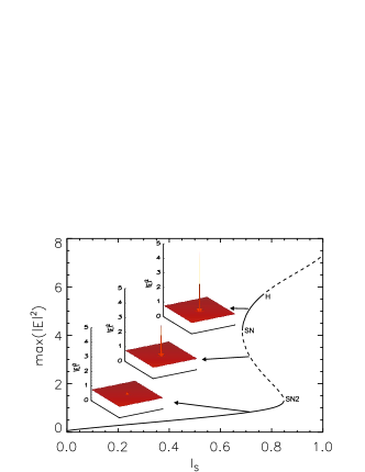
Figure 1: (Color online) Bifurcation diagram, $max(I)$ vs $I_{s}$, for a CS for $I_{sh}=0.3$, $\theta=1.25$. Solid lines represent stable solutions and dashed lines unstable ones. The insets show the transverse profile of the solutions.

One of the main consequences of the application of a localized pump is the breaking of the translational symmetry of Eq. (1). Solutions are now pinned in the region in which the Gaussian pump is applied. This also affects the transverse profile of the solutions, in particular the fundamental solution is no longer spatially homogeneous but it exhibits a bump as illustrated by the lower inset in Fig. 1.

To understand better the effects of the application of a localized pump, a diagram like the one shown in Fig. 2 of Ref. Gomila et al. (2007), that represents the maximum intensity of the transverse field as a function of $I_{s}$ is shown in Fig. 1, namely for $I_{sh}=0.3$ and $\theta=1.25$. The diagram, with three branches, looks qualitatively equivalent to the case of a homogeneous pump and operations such as switching on and off the CS can be performed in a similar way. For example, with the system at the fundamental solution, the upper branch CS can be switched on by applying an additional transient localized beam or equivalently by temporarily increasing $I_{sh}$

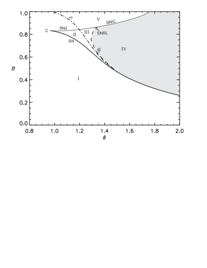
Figure 2: Two-parameter $I_{s}$ vs. $\theta$ phase diagram for $I_{sh}=0.3$. Bifurcation lines are: SN (Saddle-Node); H (Hopf); SL (Saddle-Loop); SNIC (Saddle-Node on the Invariant Circle); SN2 (Saddle-Node off invariant cycle). Regions delimited by bifurcation lines are as follows. I: only the fundamental solution is stable; II: stationary stable CS coexisting with the fundamental one; III: oscillating CS (or oscillons), coexisting with the fundamental solution; IV: excitable region; V: oscillating CS (with no other coexisting solution).

A relevant difference is that for an homogeneous pump the lowest branch (homogeneous solution) extends until the MI at $I_{s}=1$, while in the case considered here the fundamental solution merges with the middle branch CS before the MI, in a saddle-node bifurcation (that happens at $I_{s}=0.8479$, SN point in Fig. 1). To understand qualitatively this phenomenon one has to take into account that the homogeneous pump case has many symmetries, some of which are broken when a localized pump is applied. In technical parlance one says that the bifurcation has become imperfect (see, e.g., Strogatz (1994), with the consequence that a gap in $I_{s}$ appears making the lower branch disconnected in two branches (the right part of the branch is not plotted in Fig. 1 and correspond to solutions unstable to extended patterns).

Exploring now the upper branches, in Fig. 1 past the saddle-node bifurcation at $I_{s}=0.6857$ (SN point), a pair of stationary (stable, upper branch, and unstable, middle branch) localized solutions in the form of CS are found. In this parameter region, these structures are not essentially different to the solutions found in the homogeneous case Gomila et al. (2007). Increasing $I_{s}$ the stable high-amplitude CS undergoes a Hopf bifurcation.

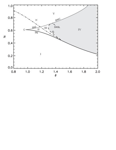
Figure 3: Two-parameter $I_{s}$ vs. $\theta$ phase diagram for $I_{sh}=0.7$. Line and region labeling as in Fig. 2.

Overall, the scenario found for a localized pump is much more involved than in the case of the homogeneous case, and more types of behavior are found in this case. Fig. 2 shows a phase diagram for a fixed value of the localized pump $I_{sh}=0.3$. One can compare this figure with Fig. 1 in Ref. Gomila et al. (2007), corresponding to $I_{sh}=0$. The effect of breaking the translational symmetry would be to unfold some of the lines at $I_{s}=1$ (not visible in Fig. 1 of Ref. Gomila et al. (2007)), that are degenerate with the MI line, and also make the SN line end at $I_{s}<1$ (point C in Fig. 2). Thus, the effect of a localized pump is to push down the SN2-SNIC line (to be explained later), as is clear from Fig. 3, that provides a similar plot for $I_{sh}=0.7$.

Some of the most prominent features of these figures, comparing with the homogeneous pump case, associated to the appearance of the SNIC line (to be discussed in more detail in Sec. IV) are that the excitable region, IV in Figs. 2-3, can have two types of excitable behavior (see Sec. V), both of Class I, as two different transitions to oscillatory behavior are possible, saddle-loop (SL) and SNIC. In addition, one has a new region, V, in which one has a single attractor in the system, that is oscillatory, to be distinguished from region III, in which the system exhibits bistability , between the (stationary) fundamental solution and an oscillatory upper branch CS. These behaviors, and how they are organized by three codimension-$2$ points will the subject of Sections VI-VII.

IV Saddle-node on the invariant circle bifurcation

A saddle-node on the invariant circle bifurcation (SNIC), also known as saddle-node infinite-period (SNIPER) and as saddle-node central homoclinic bifurcation, is a special case of a saddle-node bifurcation that occurs inside a limit cycle. Although this bifurcation is local in (one-dimensional) flows on the circle, it has global features in higher-dimensional dynamical systems Strogatz (1994), so it is also termed local-global or semilocal. In particular, the (stable) manifolds of the saddle and node fixed points transverse to the center manifold are organized by an unstable focus inside the limit cycle. At one side of the bifurcation the system exhibits oscillatory behavior, while at the other side the dynamics of the system is excitable. This mechanism leading to excitability has been found in several (zero dimensional) optical systems Coullet et al. (1998); Giudici et al. (1997); Goulding et al. (2007).

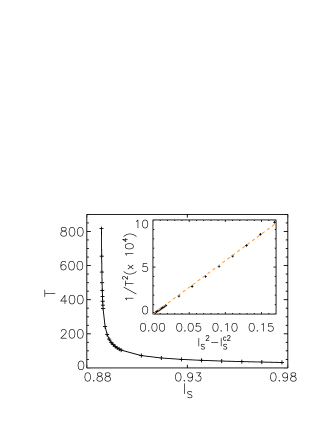
Figure 4: Period of the limit cycle $T$ as a function of $I_{s}$ for $I_{sh}=0.3$ and $\theta=1.45$. Inset: $1/T^{2}$ vs. $I_{s}$ close to the bifurcation point.

When approaching the bifurcation from the oscillatory side the period lengthens and becomes infinite. Quantitatively the period as a function of a parameter exhibits a inverse square root singular law Strogatz (1994),

$$T \propto [I_{s}^{2}-(I^{c}_{s})^{2}]^{-1/2}\ .$$ (4)

This can be used to distinguish the SNIC from other bifurcations leading to oscillatory behavior (e.g. from the saddle-loop bifurcation with a logarithmic singular law Gomila et al. (2005, 2007); Strogatz (1994)). Fig. 4 shows the period of the oscillations as a function of $I_{s}$ obtained by numerical simulations of Eq. (1). In the inset of Fig. 4 we plot $1/T^{2}$ vs. $I_{s}^{2}$ close to the bifurcation point. The linear dependence obtained corroborates the scaling law and that the transition takes place through a SNIC bifurcation.

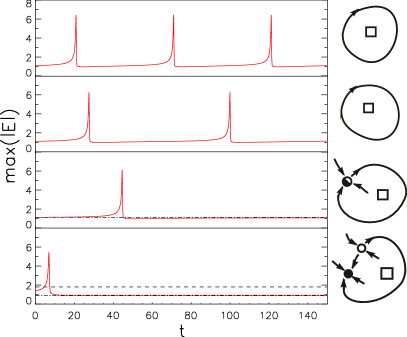
Figure 5: (Color Online) Time evolution of the CS amplitude for $I_{sh}=0.3$, $\theta=1.45$ and decreasing values of $I_{s}$ . From top to bottom, $I_{s}=0.927,0.907,0.8871,0.8$. In the bottom panel the dashed line corresponds to the amplitude of the unstable CS (saddle) while dot-dashed line corresponds to the stable fundamental solution. These two solutions coincide when the SNIC bifurcation takes place (third panel). The sketches on the right illustrate the phase space dynamics.

The overall route exhibited by the system along a vertical cut in Fig. 2 at $\theta=1.45$ is illustrated in Fig. 5, as the parameter $I_{s}$ is decreased from the top to the bottom of the Figure. Thus, the figure shows the transition from oscillatory behavior (top panel) to stationary (fourth panel) through the occurrence of a SNIC bifurcation (third panel). Lengthening of the period can be seen in the second panel. The sketches shown in the right column of Fig. 5 illustrate the structure of the phase space. The validity of this scenario is further reinforced with the quantitative analysis presented in Section VII.

V Excitability

An interesting aspect of this scenario is that in region IV one can have excitable behavior through two different mechanisms. On the one hand, and similarly to the behavior analyzed in Refs. Gomila et al. (2005, 2007), close enough to the SL line one has excitability if the fundamental solution is appropriately excited such that the oscillatory behavior existing beyond the SL is transiently recreated. The second mechanism takes place close to the SNIC line, where the oscillatory behavior that is transiently recreated is that of the oscillations in region V. Both excitable behaviors exhibit a response starting at zero frequency (or infinite period), as both bifurcations are mediated by a saddle, whose stable manifold is the threshold beyond which perturbations must be applied to excite the system. In neuroscience terminology, both excitable behaviors are class (or type) I Izhikevich (2000, 2007), although there are important differences between them. The SNIC mediated excitability is easier to observe than the one associated to a saddle-loop bifurcation for two reasons. First, it occurs in a broader parameter range due to its square-root scaling law (4), with respect to the SL excitability . Second the excitable threshold can be controlled by the intensity of the localized Gaussian beam, that effectively approaches the fixed point and the saddle in phase space, allowing to reduce the threshold as much as desired (by approaching the SNIC line). Within region IV one can find a typical crossover behavior for the threshold, as it increases from zero (at the SNIC line) to the (finite) value characteristic of the SL bifurcation as one approaches this line.

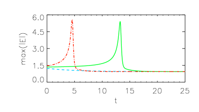
Figure 6: (Color online) Evolution of the maximum of the field amplitude after applying a localized perturbation to the fundamental solution. The perturbation has the shape of the unstable stationary CS (saddle), that is scaled by $0.95$ (blue dashed line); $1.01$ green solid line) and $1.1$ (red dotted line). Here $I_{sh}=0.3$, $I_{s}=0.8$, and $\theta=1.45$.

Fig. 6 shows the dynamics of the excitable fundamental solution in region IV, namely for the parameters corresponding to the fourth panel in Fig. 5, upon the application of different localized perturbations, one below the excitable threshold and two above. As expected, the perturbation below threshold relaxes directly to the fundamental solution while the above threshold perturbations elicit first a large response of the system in the form of an excitable soliton which finally relaxes to the fundamental solution. The excitable excursion takes place at a later time as the smaller is the distance to the threshold (a signature of Class I excitability). Finally, the shape of an excitable excursion in two-dimensional space is shown in Fig. 7.

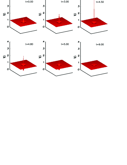
Figure 7: (Color online) Transverse profile of $|E|$ at different times of the dotted line in Fig. 6.

VI Cusp codimension-$2$ point

In the two-parameter phase diagrams in Figs. 2-3 one can see a point marked with a ’C’ that was not found in the homogeneous case . This point represents a Cusp codimension-$2$ bifurcation point Kuznetsov (2004), namely a point in which two saddle-node curves merge. This cusp point, that involves only stationary (saddle-node) bifurcations, is also known as the Cusp Catastrophe Poston and Stewart (1979). For parameter values just at the left of the Cusp the bump of the fundamental solution exhibits a rapid increase. Fig. 8 shows the sharp, but smooth, change in the shape of the fundamental solution for three parameter values around the cusp point within region I. Instead, if one is to the right of the ’C’ point this increase cannot be accommodated smoothly and a double fold occurs, such that three branches appear: two stable, upper and lower branches, and one unstable, middle branch, and thus bistability makes its appearance. The two folds, codim-$1$, merge critically at the cusp point, codim-$2$. Decreasing $I_{sh}$ the Cusp moves up towards $I_{s}=1$, so in the limit of homogeneous pump it can not be seen due to the presence of the MI instability. The smooth connection between the fundamental branch and the upper branch exhibiting CS is an outcome of the symmetry breaking induced by the localized pump which has made the MI bifurcation to become imperfect.

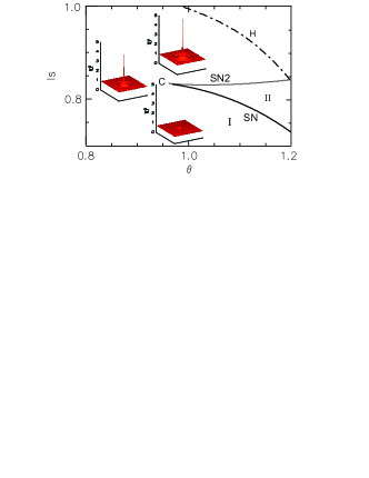
Figure 8: (Color online) The fundamental solution for three points in the $(I_{s},\theta)$ parameter space, for $I_{sh}=0.3$, around the Cusp codimension-$2$ point. The coordinates are (bottom to top): $I_{sh}=0.7,\theta=0.9$; $I_{sh}=0.85,\theta=0.85$, $I_{sh}=0.95,\theta=0.95$.

VII Saddle-node separatrix-loop codimension-$2$ point

The subject of the present section is to discuss the point designated with ’SNSL’ (that stands for Saddle-Node Separatrix Loop Schecter (1987); Izhikevich (2000) (also called Saddle-Node noncentral Homoclinic bifurcation and saddle-node homoclinic orbit bifurcation Izhikevich (2007)) in Figs. 2-3. A SNSL is a local-global codimension-$2$ point in which a saddle-node bifurcation takes place simultaneously to a saddle-loop, such that the orbit enters through the noncentral (stable) manifold. The unfolding of a SNSL point leads to the scenario depicted in Fig. 9. There is a line of saddle-node bifurcations (in which a pair of stable/unstable fixed points are created) that at one side of the SNSL is a saddle-node bifurcation off limit cycle (SN2) while at the other side is a SNIC bifurcation (the saddle-node occurs inside the limit cycle). A saddle-loop (SL) bifurcation also unfolds from the SNSL point, tangent to the SN2 line. From the other side, a special curve depicted with a dotted line in Fig. 9 should appear (cf. Fig. 22 in Ref. Izhikevich (2000)). It is not a bifurcation line, but instead it is a special line in which the approach to the node point is through the most stable direction, namely the direction transverse to the central manifold at the SNIC/SN2 (and SNSL) bifurcations (for these reasons we also call this dotted line the ’pseudo-bifurcation’ line). This, in principle nongeneric, curve, that emerges in the unfolding of the SNSL point, is necessary for consistency on the excursions around the SNSL codimension-$2$ point. At the pseudo-bifurcation the topological cycle is reconstructed, namely the stable fundamental solution and the middle branch CS (saddle), become points belonging to the circle that latter will become the limit cycle. Before the pseudo-bifurcation the unstable manifold of the saddle enters towards the stable solution from the same side than the saddle, while after the pseudo-bifurcation it enters from the opposite side.

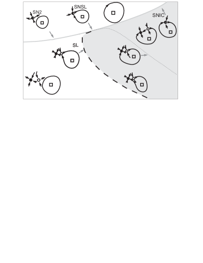
Figure 9: Sketch of the parameter space near the SNSL point, showing the unfolding of bifurcation lines, and adapted to the geometry in Figs. 2-3.

The SNSL point separates two possible ways in which the system can go from oscillatory region III (where the limit cycle coexists with the stable fundamental solution) to oscillatory region V (where the fundamental solution does not exist).

Figure 10: Spectrum of the fundamental solution at the SNIC bifurcation for $I_{sh}=0.7$, $I_{s}=0.707$, and $\theta=1.34$ (close to the SNSL).

Figure 11: Transverse cut of the most stable (left) and unstable (right) eigenmodes of the linear spectrum shown in Fig.10. The solid (dashed) line indicates the real (imaginary) part of the eigenmode.

For $\theta>\theta_{\rm SNSL}$ the scenario is as described in Section IV, namely the middle and lower branches coalesce in a SNIC bifurcation. The main feature of this bifurcation is that it occurs on the limit cycle, leading to the excitable behavior of region IV. This scenario can be confirmed using the mode projection technique described in the Appendix of Ref. Gomila et al. (2007), that allows to obtain in quantitative form the phase space of an extended system (described, e.g., by a PDE), that strictly has an infinite dimension, but whose relevant dynamics is low-dimensional. In this case, like in the case of a saddle-loop bifurcation studied in Ref. Gomila et al. (2007), we will argue that there are just two modes that are relevant, at least in the region close to the SNSL codimension-$2$ point. Fig. 10 shows the spectrum of eigenvalues (linear stability analysis for the fundamental solution) at the SNIC bifurcation and close to the SNSL. The spectrum has a continuous part with eigenvalues lying along the line ${\rm Re}(\lambda)=-1$, and also a discrete part which is symmetric with the respect to this line. It turns out that there are only two eigenmodes which are localized in space, while all the other eigenmodes are spatially extended. The two localized eigenmodes correspond to the most stable mode and to the one that becomes unstable. These two modes, shown in Fig. 11, are the only relevant for the dynamics of the CS close to the stable fixed point, since the projection of a localized solution onto any of the extended modes is negligible.

Fig. 12 shows a quantitative reconstruction of the phase space. $\beta_{1}$ ($\beta_{2}$) corresponds to the amplitude of the projection of the trajectory along the unstable (most stable) eigenmode. Panel a) represents a trajectory in the excitable region IV, close to the SNSL and below the pseudo-bifurcation line. Panel b) shows a zoom of the trajectory close to the saddle (open circle) and the stable fundamental solution (filled circle). The excitable trajectory departs form the saddle and after long excursion in phase space arrives to the fundamental solution from below (that is, from the side of the saddle). Notice that while close to the fixed points the dynamics fits very well in a 2-dimensional picture, away from them the lines crosses, indicating that the full CS dynamics in phase space is not confined to a plane. Panel c) corresponds to the pseudo-bifurcation, so that the trajectory arrives at the fundamental solution along the most stable direction. Panel d) is just after the pseudo-bifurcation with the trajectory arriving from the other side. Finally panel e) corresponds to parameters in the oscillatory region V just after the SNIC bifurcation. Notice that the pseudo-bifurcation line is very close to the SNIC bifurcation since we have taken parameters close to the SNSL and at the SNSL both lines originate tangentially. As expected, the quantitative picture agrees with the qualitatively picture as one crosses the SNIC bifurcation in the right panels of Fig. 5.

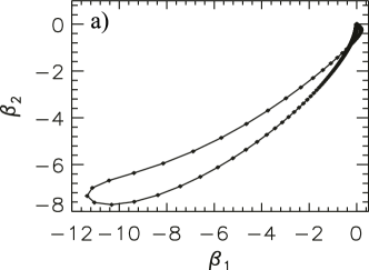
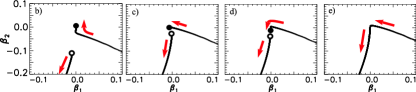
Figure 12: a) Full trajectory in the phase space close to the SNIC ($I_{s}=0.863$). The smaller panels show a zoom of the region in the phase space close to the fixed point. b) $I_{s}=0.863$, c) $I_{s}=0.8634575$, d) $I_{s}=0.8635$, and e) $I_{s}=0.864$. Here $I_{sh}=0.3$ and $\theta=1.34$.

For $\theta<\theta_{SNSL}$ the scenario is quite different, as the middle and lower branches now coalesce off the limit cycle, SN2, what implies that the behavior of the system is oscillatory on both sides of the SN2 line, not excitable and instead one crosses the SN2 line. This means that one is in a bistable oscillatory regime, and in crossing the SN2 line a saddle-node off the invariant cycle bifurcation occurs. SN2 involves the middle and fundamental branches (while SN involves the upper and middle branches). So, in the end this nothing else that another way of entering region V, of monostable oscillatory behavior, but instead of reconstructing the limit cycle, here the fundamental stationary solution is destroyed.

Therefore, and having in mind the behavior for $\theta\rightarrow\infty$ discussed in previous work for homogeneous pump Gomila et al. (2005, 2007), the overall scenario depicted in Figs. 2-3 is organized by three codimension-2 points: a Cusp point, from which two saddle-node bifurcations emerge (SN and SN2); a SNSL point from which a SNIC line emerges, and that organizes the SN2 and SL lines around; and a Takens-Bodgdanov point, occurring apparently at infinite detuning, where the SN, Hopf and SL are tangent, and that can be seen as the birth of both the Hopf and SL lines. The Takens-Bogdanov point was numerically shown to be present in the homogeneous case Gomila et al. (2005, 2007). It is reassuring that the saddle-loop bifurcation line connects two of the codimension-$2$ points, as it is not in some sense generic, and one does not expect that it emerges out of the blue sky. The scenario composed by these three codimension-2 bifurcations has been reported in other systems Mercader (2003), and from a theoretical point of view, it can be shown that it appears in the unfolding in 2-dimensional parameter space of a codimension-3 degenerate Takens-Bogdanov point Dumortier (1991).

In the limit of homogeneous pump the SN2 and SNIC lines approach the MI line at $I_{s}=1$, which, therefore, also contains the Cusp and the SNSL codimension-2 points. At the Cusp the SN (responsible for the existence of CS) originates while at the SNSL the SL (originated at the Takens-Bogdanov and responsible of the CS excitability observed for homogeneous pump) ends. Notice that for homogeneous pump close to $I_{s}=1$ azimuthal instabilities renders the CS unstable to a pattern so it is difficult to study the SN and specially the SL lines in that region. Using a localized pump and then taking the limit to homogeneous pump circumvents these limitations.

VIII Conclusions

We have presented a detailed study of the instabilities of solitons in nonlinear Kerr cavities under the application of a localized Gaussian beam. Since experimentally CS are typically switched on by applying a transient addressing beam the situation discussed here can be realized just applying it on a permanent basis. The CS are sustained by a balance between nonlinearity and dissipation, as in the case of a homogeneous pump, although now these effects interact with the localized pump. The localized pump helps to spatially fixed the CS and to control some of its dynamical properties. After the saddle-node bifurcation that creates the CS, it starts oscillating and overall exhibit a plethora of bifurcations that are shown to be organized by three codimension-$2$ points: a Takens-Bogdanov point, (which is also present for homogeneous pump as discussed already in Gomila et al. (2005, 2007)), a Cusp, and a Saddle-Node Separatrix Loop (SNSL) points. In this scenario a saddle-loop bifurcation connects the Takens-Bogdanov and the SNSL and the Cusp is connected to the other codimension-2 bifurcations by two saddle-node lines. A line of SNIC bifurcations originates at the SNSL while at the Takens-Bogdanov a Hopf bifurcation line meets tangentially a saddle-node and the saddle-loop lines.

The simultaneously presence in the system of two bifurcations that are associated to excitable behavior (saddle-loop and SNIC) enriches and completes the picture discussed for the case of a homogeneous pump. In fact the region for which excitable behavior is reported, in which the only attractor in the system is the fundamental solution, leads to two different Class I behaviors (starting at infinite period). In the excitable region one goes smoothly from no threshold at the onset of the SNIC line to a finite threshold at the onset of the saddle-loop line. In fact, the excitable behavior mediated by a SNIC, and reported in this work, should be easier to observe both numerically and experimentally, and present some practical features that make it more suitable for practical applications. In particular, the excitable threshold can be controlled by the intensity of the localized beam. With an array of properly engineered beams, created for instance with a spatial light modulator, one could create reconfigurable arrays of coupled excitable units to all-optically process information. Work in this direction will be reported elsewhere.

- (1)
- Koga and Kuramoto (1980) S. Koga and Y. Kuramoto, Prog. Theor. Phys. 392, 106 (1980).
- Kerner and Osipov (1994) B. S. Kerner and V. V. Osipov, Autosolitons: A new approach to problems of self-organization and Turbulence (Kluwer, Dordrecht, 1994).
- Vanag and Epstein (2007) V. K. Vanag and I. R. Epstein, Chaos 17, 037110 (2007).
- Niedernostheide et al. (1992) F. J. Niedernostheide, B. S. Kerner, and H. G. Purwins, Phys. Rev. B 46, 7559 (1992).
- Umbanhowar et al. (1996) P. B. Umbanhowar, F. Melo, and H. L. Swinney, Nature 382, 793 (1996).
- Niemela et al. (1990) J. J. Niemela, G. Ahlers, and D. S. Cannell, Phys. Rev. Lett. 64, 1395 (1990).
- Batiste and Knobloch (2005) O. Batiste and E. Knobloch, Phys. Rev. Lett. 95, 244501 (2005).
- Lejeune et al. (2002) O. Lejeune, M. Tlidi, and P. Couteron, Phys. Rev. E 66, 010901(R) (2002).
- Firth and Weiss (2002) W. J. Firth and C. O. Weiss, Opt. Photon. News 13, 55 (2002).
- Lugiato (2003) Feature section on cavity solitons, L.A. Lugiato ed., IEEE J. Quant. Elect. 39, #2 (2003).
- Rosanov (2002) N. N. Rosanov, Spatial Hysteresis and Optical Patterns, Springer series in synergetics (Springer, Berlin, 2002).
- Barland and et al. (2002) S. Barland et al., Nature (London) 419, 699 (2002).
- Tanguy et al. (2008) Y. Tanguy, T. Ackemann, W. J. Firth, and R. Jäger, Phys. Rev. Lett. 100, 013907 (2008).
- Tlidi et al. (2007) M. Tlidi, M. Taki, and T. Kolokolnikov, Chaos 17, 037101 (2007).
- Akhmediev and Ankiewicz (2005) N. Akhmediev and A. Ankiewicz, eds., Dissipative Solitons, vol. 661 of Lecture Notes in Physics (Springer, Berlin, 2005).
- Akhmediev and Ankiewicz (2008) N. Akhmediev and A. Ankiewicz, eds., Dissipative Solitons: From Optics to Biology and Medicine, vol. 751 of Lecture Notes in Physics (Springer, Berlin, 2008).
- Coullet et al. (2004) P. Coullet, C. Riera, and C. Tresser, Chaos 14, 193 (2004).
- Fauve and Thual (1990) S. Fauve and O. Thual, Phys. Rev. Lett. 64, 282 (1990).
- Tlidi et al. (1994) M. Tlidi, P. Mandel, and R. Lefever, Phys. Rev. Lett. 73, 640 (1994).
- Firth et al. (1996) W. J. Firth, A. Lord, and A. J. Scroggie, Phys. Scr. T67, 12 (1996).
- Firth et al. (2002) W. J. Firth, G. K. Harkness, A. Lord, J. McSloy, D. Gomila, and P. Colet, J. Opt. Soc. Am. B 19, 747 (2002).
- Vanag and Epstein (2004) V. K. Vanag and I. R. Epstein, Phys. Rev. Lett. 92, 128301 (2004).
- Gomila et al. (2005) D. Gomila, M. A. Matías, and P. Colet, Phys. Rev. Lett. 94, 063905 (2005).
- Gomila et al. (2007) D. Gomila, A. Jacobo, M. A. Matías, and P. Colet, Phys. Rev. E 75, 026217 (2007).
- Lugiato and Lefever (1987) L. A. Lugiato and R. Lefever, Phys. Rev. Lett. 58, 2209 (1987).
- Firth and Lord (1996) W. J. Firth and A. Lord, J. Mod. Opt. 43, 1071 (1996).
- Rasmussen and Rypdal (1986) J. Rasmussen and K. Rypdal, Phys. Scr. 33, 481 (1986).
- Gomila and Colet (2003) D. Gomila and P. Colet, Phys. Rev. A 68, 011801(R) (2003).
- Gomila and Colet (2007) D. Gomila and P. Colet, Phys. Rev. E 76, 016217 (2007).
- Strogatz (1994) S. H. Strogatz, Nonlinear Dynamics And Chaos (Addison-Wesley, Reading, MA, 1994).
- Coullet et al. (1998) P. Coullet, D. Daboussy, and J. R. Tredicce, Phys. Rev. E 58, 5347 (1998).
- Giudici et al. (1997) M. Giudici, C. Green, G. Giacomelli, U. Nespolo, and J. R. Tredicce, Phys. Rev. E 55, 6414 (1997).
- Goulding et al. (2007) D. Goulding, S. P. Hegarty, O. Rasskazov, S. M. M. Hartnett, G. Greene, J. G. McInerney, D. Rachinskii, and G. Huyet, Phys. Rev. Lett. 98, 153903 (2007).
- Izhikevich (2000) E. M. Izhikevich, Int. J. Bifurcation Chaos Appl. Sci. Eng. 10, 1171 (2000).
- Izhikevich (2007) E. M. Izhikevich, Dynamical Systems in Neuroscience (MIT Press, Cambridge (MA), 2007).
- Kuznetsov (2004) Y. A. Kuznetsov, Elements of Applied Bifurcation Theory, 3rd ed. (Springer-Verlag, Berlin, 2004).
- Poston and Stewart (1979) T. Poston and I. Stewart, Catastrophe Theory and its Applications (Longman, Essex, 1979).
- Schecter (1987) S. Schecter, SIAM J. Math. Anal. 18, 1142 (1987).
- Mercader (2003) E. Meca, I. Mercader, O. Batiste, L. Ramírez-Piscina, Theoret. Comput. Fluid Dynamics 18, 231 (2004). See also references therein.
- Dumortier (1991) F. Dumortier, R. Roussarie, J. Sotomayor, H. Zoladek. Bifurcations of Planar Vector Fields. Nilpotent Singularities and Abelian Integrals, Lecture Notes in Mathematics 1480, (Springer-Verlag, Berlin, 1991).