Semi-numerical power expansion of Feynman integrals

Abstract

I present an algorithm based on sector decomposition and Mellin-Barnes techniques to power expand Feynman integrals. The coefficients of this expansion are given in terms of finite integrals that can be calculated numerically. I show in an example the benefit of this method for getting the full analytic power expansion from differential equations by providing the correct ansatz for the solution. For method of regions the presented algorithm provides a numerical check, which is independent from any power counting argument.

I Introduction

For power expanding Feynman integrals several methods exist, where all of them have their limitations. Mellin-Barnes techniques provides a very general method to obtain all powers Greub:1996tg ; Smirnov:2002pj . This method however fails if the integrals are getting too complex. On the other hand method of regions Smirnov:2002pj ; Gorishnii:1989dd ; Beneke:1997zp ; Smirnov:1990rz is a convenient way to obtain the leading power, whereas it is getting rather complicated for higher powers because of the many contributing regions and because it is difficult to automatize. Furthermore it is a very non-trivial task to make sure that one has not forgotten or counted twice any region. However in the Euclidean limit, where no collinear divergences arise, automatizations exist, which rely on graph theory Chetyrkin:1996my ; Seidensticker:1999bb . Another way to expand Feynman integrals, which has been proposed and worked out in Remiddi:1997ny ; Pilipp:2007wm ; Pilipp:2007mg ; Boughezal:2007ny , is based on differential equations. Differential equation techniques, which has been proposed first in Kotikov:1990kg , is easy to automatize in a computer algebra system. This makes it a convenient method to obtain subleading powers, whereas the leading power is in most cases needed as an input like a boundary condition. Another limitation is the fact that this method relies on a correct ansatz in terms of powers of the expansion parameter. However it is a priori not obvious which powers of the expansion parameter occur (e.g. only integer powers or also half-integer powers).

In the present paper I present a semi-numerical method, that provides the power expansion of Feynman integrals by giving explicit expressions of the expansion coefficients in form of finite integrals the can be solved numerically. In particular this method gives the contributing powers of the expansion parameter, from where one can read off the correct ansatz to solve the differential equations that determine the set of Feynman integrals.

The algorithm that is worked out in the present paper combines sector decomposition Binoth:2000ps ; Heinrich:2002rc ; Binoth:2003ak ; Heinrich:2008si with Mellin-Barnes techniques. It is completely independent from any power counting argument such that it can be used as a cross check for method of regions. This is very useful in cases, where method of regions becomes involved because of many contributing regions.

The paper is organized as follows. In Section II the algorithm is explained in detail. In Section III I apply this algorithm to a set of two Feynman integrals, that are power expanded by differential equation techniques, where the leading powers are obtained by method of regions. I will show explicitly how this algorithms gives the correct ansatz for the differential equations and provides a non-trivial check for method of regions.

II Algorithm

We follow the steps of Section 2 of Binoth:2000ps . We start with a $L$-Loop Feynman integral

$$G=\int\prod_{i=1}^{L}\frac{d^{D}k_{i}}{(2\pi)^{D}}\frac{1}{P_{1}\ldots P_{N}}$$ (1)

which using the Feynman parameterization

$$\frac{1}{P_{1}\ldots P_{N}}=\Gamma(N)\int_{0}^{1}d^{N}x\,\frac{\delta\left(1-\sum_{n=1}^{N}x_{n}\right)}{\left(x_{1}P_{1}+\ldots+x_{N}P_{N}\right)^{N}}$$ (2)

can be cast into the form:

$$G=\Gamma(N)\int d^{N}x\,\delta(1-\sum_{n=1}^{N}x_{n})\int\prod_{i=1}^{L}\frac{d^{D}k_{i}}{(2\pi)^{D}}\left[\sum_{j,l=1}^{L}k_{j}\cdot k_{l}M_{jl}-2\sum_{j=1}^{L}k_{j}\cdot Q_{j}+J\right]^{-N}.$$ (3)

We define $D=4-2\epsilon$ as usual. After performing the integration over the loop momenta we obtain:

$$G=(-1)^{N}\left(\frac{i}{(4\pi)^{D/2}}\right)^{L}\Gamma(N-LD/2)\int d^{N}x\,\delta(1-\sum_{n=1}^{N}x_{n})\frac{U^{N-(L+1)D/2}}{F^{N-LD/2}},$$ (4)

where

$$F=-\det(M)\left[J-\sum_{j,l=1}^{L}Q_{j}\cdot Q_{l}M_{jl}^{-1}\right]$$ (5)

and

$$U=\det(M).$$ (6)

Let us assume (5) contains the parameter $\lambda$, in which we want to expand (3). Using the Mellin-Barnes representation Smirnov:2002pj

$$\frac{1}{(X_{1}+X_{2})^{x}}=\frac{1}{\Gamma(x)}\frac{1}{2\pi i}\int_{-i\infty}^{i\infty}ds\,\Gamma(-s)\Gamma(s+x)X_{1}^{s}X_{2}^{-s-x},$$ (7)

where the integration contour over $s$ has to be chosen such that

$$-x<\Re(s)<0,$$

we modify (4) in the following way

$$\begin{split}G=&(-1)^{N}\left(\frac{i}{(4\pi)^{D/2}}\right)^{L}\frac{1}{2\pi i}\int_{-i\infty}^{i\infty}ds\,\lambda^{s}\Gamma(-s)\Gamma(s+N-LD/2)\\ &\times\int d^{N}x\,\delta(1-\sum_{n=1}^{N}x_{n})U^{N-(L+1)D/2}F_{1}^{s}F_{2}^{-s-N+LD/2},\end{split}$$ (8)

where

$$F=\lambda F_{1}+F_{2}.$$ (9)

The main idea behind the procedure below is the following: By closing the integration path to the right hand side of the imaginary axis we sum up all the residua on the positive real axis and obtain an expansion in $\lambda$. Powers of $\ln\lambda$ appear because of poles of order higher than one and because of terms of the form $\lambda^{A-B\epsilon}$ in the expansion in $\lambda$. These terms turn after expanding in $\epsilon$ into powers of $\ln\lambda$.

We continue with part I and II of Binoth:2000ps . First we split the integral over the Feynman parameters into

$$\int d^{N}x=\sum_{l=1}^{N}\int d^{N}x\prod_{\stackrel{{\scriptstyle j=1}}{{j\neq l}}}^{N}\theta(x_{l}-x_{j})$$ (10)

and integrate out the $\delta$-function by the substitution

$$x_{j}=\left\{\begin{array}[]{l@{\quad}l}x_{l}t_{j}&j<l\\ x_{l}&j=l\\ x_{l}t_{j-1}&j>l\end{array}\right.$$ (11)

such that we obtain

$$G=(-1)^{N}\left(\frac{i}{(4\pi)^{D/2}}\right)^{L}\frac{1}{2\pi i}\int_{-i\infty}^{i\infty}ds\,\lambda^{s}\Gamma(-s)\Gamma(s+N-LD/2)\sum_{l=1}^{N}\int_{0}^{1}d^{N-1}t\,G_{l},$$ (12)

where

$$G_{l}=U_{l}^{N-(L+1)D/2}F_{1,l}^{s}F_{2,l}^{-s-N+LD/2}$$ (13)

is obtained by the substitution (11). In (12) the integration over small $t$ leads to poles in $s$. This behavior is made explicit, if we follow the steps of Part II of Binoth:2000ps : Look for a minimal set $\{t_{\alpha_{1}},\ldots,t_{\alpha_{r}}\}$ such that $U_{l}$, $F_{1,l}$ or $F_{2,l}$ vanish, if these parameters are set to zero. We decompose the integral into $r$ subsectors

$$\int_{0}^{1}d^{N-1}t=\int_{0}^{1}d^{N-1}t\sum_{k=1}^{r}\prod_{\stackrel{{\scriptstyle j=1}}{{j\neq k}}}^{r}\theta(t_{\alpha_{k}}-t_{\alpha_{j}})$$ (14)

and substitute

$$t_{\alpha_{j}}\to\left\{\begin{array}[]{l@{\quad}l}t_{\alpha_{k}}t_{\alpha_{j}}&j\neq k\\ t_{\alpha_{k}}&j=k\end{array}\right.,$$ (15)

which leads to the Jacobian factor $t_{\alpha_{k}}^{r-1}$. Now we are able to factorize out $t_{\alpha_{k}}$ from $U_{l}$, $F_{1,l}$ or $F_{2,l}$. After repeating these steps, until $U_{l}$, $F_{1,l}$ and $F_{2,l}$ contain terms that are constant in $\vec{t}$, we end up with integrals over the Feynman parameters of the form

$$\sum_{l=1}^{N}\sum_{k}\int_{0}^{1}d^{N-1}t\left(\prod_{j=1}^{N-1}t_{j}^{A_{j}-B_{j}\epsilon-C_{j}s}\right)U_{lk}^{N-(L+1)D/2}F_{1,lk}^{s}F_{2,lk}^{-s-N+LD/2},$$ (16)

where $U_{lk}$, $F_{1,lk}$ and $F_{2,lk}$ contain terms that are constant in $\vec{t}$. The procedure above can in principal lead to infinite loops. This problem was addressed in Bogner:2007cr ; Smirnov:2008py , where algorithms are proposed that avoid these endless loops by choosing appropriate subsectors. I have not yet faced any endless loop in the problems I dealt with. However one should keep in mind that they can occur and adapt the implementation of the algorithm if needed.

From (16) we can read off that the poles in $s$ are located at:

$$s_{jn}=\frac{1+n+A_{j}-B_{j}\epsilon}{C_{j}},$$ (17)

where $n\in\mathbb{N}_{0}$. Eq. (17) becomes clear if one Taylor expands in (16) the terms outside the brackets with respect to $t_{j}$ and performs the integration.

In (12) we have to choose the contour of the integration over $s$ such that the integration over the Feynman parameters $t_{j}$ converges. This leads to the condition

$$A_{j}-B_{j}\epsilon-C_{j}\Re(s)>-1\quad\forall j.$$ (18)

The poles in (17) that have to be taken into account are those that are located on the right hand side of the integration contour, i.e.

$$\Re(s)<s_{jn}.$$ (19)

From (17) and (18) we conclude that (19) is fulfilled if and only if $C_{j}>0$.

In the next step we calculate the residue of (16) at $s_{jn}$. We write the $k$’th Feynman integral in the form

$$\int_{0}^{1}dt_{k}\,t_{k}^{A^{\prime}-B^{\prime}\epsilon-C^{\prime}(s-s_{jn})}\mathcal{I}(t_{k},s)$$ (20)

and note that this term is singular in $s-s_{jn}$ if and only if

$$B^{\prime}=0\quad\text{and}\quad A^{\prime}\leq-1.$$ (21)

So following Part III of Binoth:2000ps we expand $\mathcal{I}(t_{k},s)$ around $t_{k}=0$ and obtain

$$\mathcal{I}(t_{k},s)=\sum_{p=0}^{-A^{\prime}-1}\mathcal{I}^{(p)}(s)\frac{t_{k}^{p}}{p!}+R(t_{k},s),$$ (22)

with a rest term $R(t_{k},s)=\mathcal{O}(t^{-A^{\prime}})$, such that (20) becomes

$$\sum_{p=0}^{-A^{\prime}-1}\frac{1}{A^{\prime}+1+p-C^{\prime}(s-s_{jn})}\frac{\mathcal{I}^{(p)}(s)}{p!}+\int_{0}^{1}dt_{k}\,t_{k}^{A^{\prime}-C^{\prime}(s-s_{jn})}R(t_{k},s),$$ (23)

where we used that $B^{\prime}=0$. We repeat this procedure for all $k$ where condition (21) is fulfilled. The remaining integrals do not diverge for $s=s_{jn}$. So it is save to expand them around $s-s_{jn}$ and we can easily calculate the residue at $s=s_{jn}$.

What is left is to calculate the Laurent expansion in $\epsilon$. From the previous procedure we obtain terms of the form

$$\int_{0}^{1}d^{n}t\,\left(\prod t_{j}^{A_{j}^{\prime\prime}-B_{j}^{\prime\prime}\epsilon}(\ln t_{j})^{\alpha_{j}}\right)I(\vec{t},\epsilon)$$ (24)

The logarithms $(\ln t_{j})^{\alpha_{j}}$ arise from taking the residues of terms of the form $\frac{t_{j}^{-C^{\prime}(s-s_{jn})}}{(s-s_{jn})^{m}}$ with $m\geq 2$. In (24) we wrote these logarithms explicitly such that we can expand $I(\vec{t},\epsilon)$ around $t_{j}=0$. The poles in $\epsilon$ in (24) originate from integrals

$$\int_{0}^{1}dt_{j}\,t_{j}^{A_{j}^{\prime\prime}-B_{j}^{\prime\prime}\epsilon}(\ln t_{j})^{\alpha_{j}}\mathcal{I}(t_{j},\epsilon)$$ (25)

with $A_{j}^{\prime\prime}\leq-1$. Repeating the procedure above we expand

$$\mathcal{I}(t_{j},\epsilon)=\sum_{p=0}^{-A_{j}^{\prime\prime}-1}\mathcal{I}^{(p)}(\epsilon)\frac{t_{j}^{p}}{p!}+R(t_{j},\epsilon)$$ (26)

and obtain for (25)

$$\sum_{p=0}^{-A_{j}^{\prime\prime}-1}\frac{(-1)^{\alpha_{j}}(\alpha_{j}+1)!}{(1+p+A_{j}^{\prime\prime}-B_{j}^{\prime\prime}\epsilon)^{\alpha_{j}+1}}\frac{\mathcal{I}^{(p)}(\epsilon)}{p!}+\int_{0}^{1}dt_{j}\,t_{j}^{A_{j}^{\prime\prime}-B_{j}^{\prime\prime}\epsilon}(\ln t_{j})^{\alpha_{j}}R(t_{j},\epsilon).$$ (27)

All the remaining integrals over $t_{j}$ are finite and can in principle be calculated numerically. Finally the original integral $G$ in (3) obtains the form

$$G=\sum_{i,m,n}\epsilon^{i}\lambda^{m}(\ln\lambda)^{n}I_{i,m,n},$$ (28)

where the $I_{i,m,n}$ contain finite integrals that can be numerically evaluated. The logarithms $(\ln\lambda)^{n}$ arise both due to poles of higher order in the Mellin-Barnes parameter and to the expansion in $\epsilon$ from terms of the form $\lambda^{\epsilon}/\epsilon^{n}$. Depending on the values of $C_{j}$ in (17) the sum over $m$ does not only run over integer numbers but also over numbers of the form

$$\frac{1+n+A_{j}}{C_{j}},$$

where $n$ is integer. I stress that even if a numerical evaluation of the integrals $I_{i,m,n}$ is not possible, we can obtain non-trivial statements about the power expansion of $G$ from (28) together with (17). That is to say (17) gives us information about the possible powers of $\lambda$ e.g. we know if we only get integer powers or also powers of $\sqrt{\lambda}$. And from (28) we can read off up to which power $\ln\lambda$ appears. As we will see in the next section this information will prove to be useful to obtain the power expansion by means of differential equations.

III Example: Power expansion of Feynman integrals by differential equation techniques

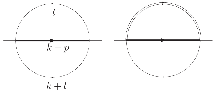
Figure 1: Sunrise diagrams. The thick line denotes a propagator of mass $M$, while the thin lines stand for mass $m$. The double line denotes that the propagator is to be taken squared.

The idea to get the expansion of Feynman integrals by differential equations has been proposed and worked out in Remiddi:1997ny ; Pilipp:2007wm ; Pilipp:2007mg ; Boughezal:2007ny . By the following example we will see that the algorithm shown in the last section will give us the correct ansatz to solve the given system of differential equations and help us with the calculation of the initial conditions. We start with the integrals given by Fig. 1, where we assume $p^{2}=M^{2}$:

$$I_{1} = \int\frac{d^{D}k}{(2\pi)^{D}}\frac{d^{D}l}{(2\pi)^{D}}\frac{1}{(k^{2}+2k\cdot p)\left((k+l)^{2}-m^{2}\right)\left(l^{2}-m^{2}\right)}$$

$$I_{2} = \int\frac{d^{D}k}{(2\pi)^{D}}\frac{d^{D}l}{(2\pi)^{D}}\frac{1}{(k^{2}+2k\cdot p)\left((k+l)^{2}-m^{2}\right)\left(l^{2}-m^{2}\right)^{2}}.$$ (29)

Let us assume that we want to expand these integrals in $\lambda=m^{2}/M^{2}$ and need the result up to order $\mathcal{\epsilon}$. For simplicity let us also set $M^{2}=1$ and $m^{2}=\lambda$. Using integration-by-parts identities Chetyrkin:1981qh ; Tkachov:1981wb ; Laporta:2001dd , we get the following differential equations for $I_{1}$ and $I_{2}$:

$$\frac{d}{d\lambda}I_{1} = h_{11}I_{1}+h_{12}I_{2}+g_{1}$$

$$\frac{d}{d\lambda}I_{2} = h_{21}I_{1}+h_{22}I_{2}+g_{2}$$ (30)

with

$$h=\left(\begin{array}[]{cc}0&2\\ \frac{1}{2\lambda(1-\lambda)}&\frac{1-3\lambda}{2\lambda(1-\lambda)}\end{array}\right)+\epsilon\left(\begin{array}[]{cc}0&0\\ -\frac{7}{4\lambda(1-\lambda)}&\frac{-2+4\lambda}{\lambda(1-\lambda)}\end{array}\right)+\epsilon^{2}\left(\begin{array}[]{cc}0&0\\ 0&\frac{3}{2\lambda(1-\lambda)}\end{array}\right)$$ (31)

and

$$g_{1} = 0$$

$$g_{2} = \frac{(1-\epsilon)^{2}}{4\lambda^{2}(1-\lambda)}\bigg{[}\int\frac{d^{D}k}{(2\pi)^{D}}\frac{d^{D}l}{(2\pi)^{D}}\frac{1}{\left((k+l)^{2}-\lambda\right)\left(l^{2}-\lambda\right)}-$$ (32)

$$\int\frac{d^{D}k}{(2\pi)^{D}}\frac{d^{D}l}{(2\pi)^{D}}\frac{1}{(k^{2}+2k\cdot p)\left(l^{2}-\lambda\right)}\bigg{]}$$

$$= \frac{1}{(4\pi)^{D}}\Gamma(\epsilon)^{2}\frac{\lambda^{1-2\epsilon}-\lambda^{-\epsilon}}{4\lambda(1-\lambda)},$$

where (31) and (32) are exact in $\lambda$ and $\epsilon$. By defining

$$I_{\alpha} = \sum_{i,j,k}I_{\alpha,i}^{(j,k)}\epsilon^{i}\lambda^{j}(\ln\lambda)^{k}$$

$$h_{\alpha\beta} = \sum_{i,j}h_{\alpha\beta,i}^{(j)}\epsilon^{i}\lambda^{j}$$

$$g_{\alpha} = \sum_{i,j,k}g_{\alpha,i}^{(j,k)}\epsilon^{i}\lambda^{j}(\ln\lambda)^{k}$$ (33)

(30) becomes

$$0=(j+1)I_{\alpha,i}^{(j+1,k)}+(k+1)I_{\alpha,i}^{(j+1,k+1)}-\sum_{\beta=1,2}\sum_{i^{\prime}=0}^{2}\sum_{j^{\prime}=-1}^{j}h_{\alpha\beta,i^{\prime}}^{(j^{\prime})}I_{\beta,i-i^{\prime}}^{(j-j^{\prime},k)}-g_{\alpha,i}^{(j,k)}.$$ (34)

In (33) we have not yet specified which values the summation index $j$ takes and up to which maximum value the finite sum over $k$ runs. By implementing the steps of the last section, which led to (17), in a computer algebra system we obtain from (17) that $I_{1}$ comes with the powers of $\lambda$

$$\lambda^{n},\quad\lambda^{n+1-\epsilon},\quad\lambda^{\frac{n+3}{2}-2\epsilon}$$ (35)

and $I_{2}$ with

$$\lambda^{n},\quad\lambda^{n-\epsilon},\quad\lambda^{\frac{n+1}{2}-2\epsilon},$$ (36)

where $n\in\mathbb{N}_{0}$. From (35) and (36) we read off that $j$ takes the values $0,1/2,1,\ldots$. In (34) integer-valued and half-integer-valued $j$ do not mix. So we would have missed powers of $\sqrt{\lambda}$, if we had made the naïve ansatz that $I_{1,2}$ only come with integer powers of $\lambda$. Now one could argue that $\sqrt{\lambda}$ is already contained in the sum over $\ln\lambda$. However in order to solve (34) we have to assume that there exists $k_{\text{max}}$ such that $I^{(j,k)}_{\alpha,i}=0$ for all $k>k_{\text{max}}$. A computer algebra analysis of the algorithm in the previous section tells us that in our special case $k_{\text{max}}=3$.

Solving (34) up to $\mathcal{O}(\epsilon)$ we note that we need $I_{1,i}^{(0,0)}$ and $I_{2,i}^{(\frac{1}{2},0)}$ as initial conditions, which can be obtained by method of regions Smirnov:2002pj ; Gorishnii:1989dd ; Beneke:1997zp ; Smirnov:1990rz . In the case of $I_{1,i}^{(0,0)}$ we note that only the region participates where both integration momenta are hard:

$$k^{\mu}=\mathcal{O}(1)\quad\text{and}\quad l^{\mu}=\mathcal{O}(1).$$ (37)

In this region we obtain

$$\int\frac{d^{D}k}{(2\pi)^{D}}\frac{d^{D}l}{(2\pi)^{D}}\frac{1}{(k^{2}+2k\cdot p)(k+l)^{2}l^{2}}=\frac{1}{(4\pi)^{D}}\frac{\Gamma(-1+2\epsilon)\Gamma(\epsilon)\Gamma(1-\epsilon)^{2}\Gamma(3-4\epsilon)}{\Gamma(2-2\epsilon)\Gamma(3-3\epsilon)},$$ (38)

which is the leading power of $I_{1}$. For $I_{2,i}^{(\frac{1}{2},0)}$ we need the region where both $k$ and $l$ are soft, i.e.

$$k^{\mu}=\mathcal{O}(\sqrt{\lambda})\quad\text{and}\quad l^{\mu}=\mathcal{O}(\sqrt{\lambda}).$$ (39)

This region starts participating at $\mathcal{O}(\sqrt{\lambda})$:

$$\begin{split}&\int\frac{d^{D}k}{(2\pi)^{D}}\frac{d^{D}l}{(2\pi)^{D}}\frac{1}{(2k\cdot p)\left((k+l)^{2}-\lambda\right)\left(l^{2}-\lambda\right)^{2}}=\\ &\quad\quad\frac{-1}{(4\pi)^{D}}\frac{2^{-2\epsilon}\pi\Gamma\left(\epsilon-\frac{1}{2}\right)\Gamma\left(2\epsilon-\frac{1}{2}\right)}{\Gamma(\epsilon)}\lambda^{\frac{1}{2}-2\epsilon}.\end{split}$$ (40)

By comparing these results to (35) and (36) we note that (38) and (40) correspond to definite poles in the Mellin-Barnes representation i.e. at $s=0$ and $s=1/2-2\epsilon$. By (17) and (23) we can calculate the coefficients of $\lambda^{0}$ and $\lambda^{\frac{1}{2}-2\epsilon}$ in the $\lambda$-expansion of $I_{1}$ and $I_{2}$ numerically. This is a non-trivial test that we have not forgotten a contributing region, which is in general a problem of method of regions.

We normalize our integrals by multiplication with $(\exp(\gamma_{\text{E}})/(4\pi))^{2\epsilon}$ and obtain from the solution of (34) the analytical expansion in $\lambda$ and $\epsilon$:

$$\begin{split}&I_{1}=\\ &\quad\quad\frac{1}{(4\pi)^{4}}\bigg{[}-\frac{1}{2\epsilon^{2}}-\frac{5}{4\epsilon}-\frac{11}{8}-\frac{5\pi^{2}}{12}+\epsilon\left(\frac{55}{16}-\frac{25\pi^{2}}{24}-\frac{11}{3}\zeta(3)\right)+\\ &\quad\quad\lambda\bigg{(}-\frac{1}{\epsilon^{2}}+\frac{-3+2\ln\lambda}{\epsilon}-5+\frac{\pi^{2}}{2}+6\ln\lambda-(\ln\lambda)^{2}+\\ &\quad\quad\quad\epsilon\left(-3+\frac{3\pi^{2}}{2}+\frac{26}{3}\zeta(3)+\left(14+\frac{\pi^{2}}{3}\right)\ln\lambda-3(\ln\lambda)^{2}+\frac{(\ln\lambda)^{3}}{3}\right)\bigg{)}+\\ &\quad\quad\lambda^{\frac{3}{2}}\epsilon\frac{-16\pi^{2}}{3}+\mathcal{O}(\lambda^{2})\bigg{]}+\mathcal{O}(\epsilon^{2})\end{split}$$

$$\begin{split}&I_{2}=\\ &\quad\quad\frac{1}{(4\pi)^{4}}\bigg{[}-\frac{1}{2\epsilon^{2}}+\frac{-1+2\ln\lambda}{2\epsilon}+\frac{1}{2}+\frac{\pi^{2}}{4}+2\ln\lambda-\frac{1}{2}(\ln\lambda)^{2}+\\ &\quad\quad\quad\epsilon\left(\frac{11}{2}+\frac{11\pi^{2}}{12}+\frac{13}{3}\zeta(3)+\left(4+\frac{\pi^{2}}{6}\right)\ln\lambda-(\ln\lambda)^{2}+\frac{1}{6}(\ln\lambda)^{3}\right)+\\ &\quad\quad\lambda^{\frac{1}{2}}(-4\epsilon\pi^{2})+\\ &\quad\quad\lambda\bigg{(}-1-\frac{\pi^{2}}{3}+\ln\lambda-\frac{1}{2}(\ln\lambda)^{2}+\\ &\quad\quad\quad\epsilon\left(11+\frac{2\pi^{2}}{3}-4\zeta(3)-3\ln\lambda-\frac{1}{2}(\ln\lambda)^{2}+\frac{1}{2}(\ln\lambda)^{3}\right)\bigg{)}+\\ &\quad\quad\lambda^{\frac{3}{2}}\epsilon\frac{4\pi^{2}}{3}+\mathcal{O}(\lambda^{2})\bigg{]}+\mathcal{O}(\epsilon^{2}).\end{split}$$ (41)

On the other hand our numeric method of Section II gives

$$\begin{split}&I_{1}=\\ &\quad\quad 10^{-4}\bigg{[}-\frac{0.20}{\epsilon^{2}}+\frac{-0.50}{\epsilon}-2.2-4.5\epsilon+\\ &\quad\quad\lambda\bigg{(}-\frac{0.40}{\epsilon^{2}}+\frac{-1.2+0.80\ln\lambda}{\epsilon}-0.026+2.4\ln\lambda-0.40(\ln\lambda)^{2}+\\ &\quad\quad\quad\epsilon\left(8.9+6.9\ln\lambda-1.2(\ln\lambda)^{2}+0.13\ln\lambda)^{3}\right)\bigg{)}-\\ &\quad\quad 21.\epsilon\lambda^{\frac{3}{2}}+\mathcal{O}(\lambda^{2})\bigg{]}+\mathcal{O}(\epsilon^{2})\end{split}$$

$$\begin{split}&I_{2}=\\ &\quad\quad 10^{-4}\bigg{[}-\frac{0.20}{\epsilon^{2}}+\frac{-0.20+0.40\ln\lambda}{\epsilon}+1.2+0.80\ln\lambda-0.20(\ln\lambda)^{2}+\\ &\quad\quad\quad\epsilon\left(7.9+2.2\ln\lambda-0.40(\ln\lambda)^{2}+0.067(\ln\lambda)^{3}\right)-\\ &\quad\quad 16.\epsilon\lambda^{\frac{1}{2}}+\\ &\quad\quad\lambda\bigg{(}-1.7+0.40\ln\lambda-0.20(\ln\lambda)^{2}+\\ &\quad\quad\quad\epsilon\left(5.1-1.2\ln\lambda-0.20(\ln\lambda)^{2}+0.20(\ln\lambda)^{3}\right)\bigg{)}+\\ &\quad\quad 5.3\epsilon\lambda^{\frac{3}{2}}+\mathcal{O}(\lambda^{2})\bigg{]}+\mathcal{O}(\epsilon^{2}),\end{split}$$ (42)

which is consistent with (41).

IV Conclusions

By combining sector decomposition with Mellin-Barnes techniques I developed an algorithm for power expanding Feynman integrals, where the coefficients in the expansion are given by finite integrals. Even if these integrals cannot be evaluated numerically, we can read off, which powers of the expansion parameter contribute and up to which power the logarithms occur. This non-trivial information provides the correct ansatz for solving the set of differential equations that determine the Feynman integrals.

Another application of the presented algorithm is testing method of regions numerically. We have seen that every region, that has a unique scaling in the expansion parameter, corresponds to a definite power in the Mellin-Barnes expansion. So it can be tested separately. For method of regions it is often an involved problem to make sure not to have missed or counted twice any region. This algorithm provides a test of method of regions that is independent of any power counting argument.

References

• (1) C. Greub, T. Hurth and D. Wyler, Phys. Rev. D54, 3350 (1996), [hep-ph/9603404].
• (2) V. A. Smirnov, Springer Tracts Mod. Phys. 177, 1 (2002).
• (3) S. G. Gorishnii, Nucl. Phys. B319, 633 (1989).
• (4) M. Beneke and V. A. Smirnov, Nucl. Phys. B522, 321 (1998), [hep-ph/9711391].
• (5) V. A. Smirnov, Commun. Math. Phys. 134, 109 (1990).
• (6) K. G. Chetyrkin, R. Harlander, J. H. Kuhn and M. Steinhauser, Nucl. Instrum. Meth. A389, 354 (1997), [hep-ph/9611354].
• (7) T. Seidensticker, [hep-ph/9905298].
• (8) E. Remiddi, Nuovo Cim. A110, 1435 (1997), [hep-th/9711188].
• (9) V. Pilipp, [arXiv:0709.0497].
• (10) V. Pilipp, Nucl. Phys. B794, 154 (2008), [arXiv:0709.3214].
• (11) R. Boughezal, M. Czakon and T. Schutzmeier, JHEP 09, 072 (2007), [arXiv:0707.3090].
• (12) A. V. Kotikov, Phys. Lett. B254, 158 (1991).
• (13) T. Binoth and G. Heinrich, Nucl. Phys. B585, 741 (2000), [hep-ph/0004013].
• (14) G. Heinrich, Nucl. Phys. Proc. Suppl. 116, 368 (2003), [hep-ph/0211144].
• (15) T. Binoth and G. Heinrich, Nucl. Phys. B680, 375 (2004), [hep-ph/0305234].
• (16) G. Heinrich, [arXiv:0803.4177].
• (17) C. Bogner and S. Weinzierl, Comput. Phys. Commun. 178, 596 (2008), [arXiv:0709.4092].
• (18) A. V. Smirnov and M. N. Tentyukov, [arXiv:0807.4129].
• (19) K. G. Chetyrkin and F. V. Tkachov, Nucl. Phys. B192, 159 (1981).
• (20) F. V. Tkachov, Phys. Lett. B100, 65 (1981).
• (21) S. Laporta, Int. J. Mod. Phys. A15, 5087 (2000), [hep-ph/0102033].