Quantum tetrahedron and its classical limit

Abstract

Classical information that is retrieved from a quantum tetrahedron is intrinsically fuzzy. We present an asymptotically optimal generalized measurement for the extraction of classical information from a quantum tetrahedron. For a single tetrahedron the optimal uncertainty in dihedral angles is shown to scale as an inverse of the surface area. Having commutative observables allows to show how the clustering of many small tetrahedra leads to a faster convergence to a classical geometry.

I Introduction

Basis states in the kinematical Hilbert space of loop quantum gravity (LQG) are represented by spin networks, which are finite, directed, labeled graphs. Their edges are labeled by SU(2) spins, and SU(2)-invariant tensors (intertwiners) label the vertices. These two families of decorations are linked to the geometric operators. A spin label attached to a link determines the area of a surface that is intersected by it, while an intertwiner is associated with the volume of a spatial region that contains the vertex. One of the major results of LQG lqg is a quantization of space: the spectrum of geometric operators representing area or volume is discrete. At present there is no rigorous proof that this result is valid in the full theory, since the geometric operators do not commute with the constraints, but there are plausible arguments that this is indeed the case. contr .

The simplest state that represents a finite volume of space involves a four-valent vertex spin network vertex. A dual picture associates vertices with tetrahedra and edges with two-dimensional surfaces, so an atom of space can be represented as a quantum tetrahedron. Its triangular areas fix the spin labels and the volume determines the intertwiner. The same mathematical structure results from a formal quantization of a classical tetrahedron tetra .

Geometry of a classical tetrahedron is determined by six parameters. This number is obtained by removing the rigid body degrees of freedom from the twelve coordinates of tetrahedron’s vertices. Six geometric variables are associated with observables on the Hilbert space ${\cal H}_{0}$ of a quantized tetrahedron. However, the maximal set of commuting observables contains only five operators, which makes a retrieved classical description intrinsically fuzzy. A coherent quantum cs tetrahedron is a useful toy model to investigate a classical limit of LQG lqg . Recently it gained importance in providing boundary states in the studies of a graviton propagator prop .

In the language of quantum information the classical limit of a quantum tetrahedron is equivalent to a faithful transmission of its shape without any knowledge of the spatial orientation. We will use quantum-informational techniques to get some insights into the classical limit.

This paper is organized as follows. In the next Section we review some properties of classical and quantum tetrahedra. Sec. III establishes an upper bound on the convergence to a sharp classical geometry. Sec. IV exhibits a generalized measurement of two parameters that correspond to the non-commuting observables. Finally, Sec. V discusses classical geometry of an aggregate of many small tetrahedra. Necessary background information about generalized measurements is given in Appendix A, while the explicit formulas are collected in Appendix B.

II Classical and quantum tetrahedra

In this Section we review some facts about classical and quantum tetra ; ct tetrahedra. There are several sets of six numbers that determine its shape. For example, one can use the six edges of a tetrahedron, or four facial areas and two independent angles between them. The latter parametrization gives a natural way to compare classical values with the estimates obtained from a quantum tetrahedron.

We label the outward normals to the faces as ${\mathbf{J}}_{i}$, and following the convention take their lengths to be twice the triangular areas, $J_{i}=2A_{i}$. Being a closed surface a tetrahedron satisfies the closure condition

$$\sum_{i=1}^{4}{\mathbf{J}}_{i}=0.$$ (1)

There is a number of useful relations between areas, angles and volume ct . Angles between the triangular faces are the (inner) dihedral angles, which are related to the outer dihedral angles $\theta_{ij}$,

$$J_{ij}\equiv{\mathbf{J}}_{i}\!\cdot{\mathbf{J}}_{j}=J_{i}J_{j}\cos\theta_{ij}$$ (2)

as $\theta_{ij}^{\mathrm{in}}=\pi-\theta_{ij}$. The volume can be expressed in terms of the area vectors,

$$V^{2}=-\frac{1}{36}\epsilon_{abc}J_{1}^{a}J_{2}^{b}J_{3}^{c}=-\frac{1}{36}{\mathbf{J}}_{1}\cdot{\mathbf{J}}_{2}\times{\mathbf{J}}_{3}.$$ (3)

and, e.g.,

$$\sin\theta_{ij}^{\mathrm{in}}=\frac{3V\,l_{ij}}{2A_{i}A_{j}},$$ (4)

where $l_{ij}$ is a length of the edge between the faces $i$ and $j$. In the following we take $J_{1}$,$J_{2}$, $J_{3}$, $J_{4}$, $\theta_{12}$ and $\theta_{23}$ to form the shape-defining set.

In the quantized problem the four normals are identified with the generators of SU(2),

$${\hat{\mathbf{J}}}^{2}_{i}|j_{i},m_{i}\rangle=j_{i}(j_{i}+1)|j_{i},m_{i}\rangle,\qquad\hat{J}_{zi}|j_{i},m_{i}\rangle=m_{i}|j_{i},m_{i}\rangle.$$ (5)

For later use we note that the Casimir operator asymptotically equals to $J\equiv\sqrt{j(j+1)}\simeq j+\mbox{$\frac{1}{2}$}{}$.

The closure constraint Eq. (1) restricts the Hilbert space to its SU(2) invariant subspace,

$${\cal H}_{0}=\bigoplus_{\{j_{k}\}}{\cal H}_{0}^{\{j_{k}\}}=\bigoplus_{\{j_{k}\}}\mathrm{Inv}\left(\bigotimes_{k=1}^{4}\mathbbm{C}^{d_{k}}\right),$$ (6)

where the dimension of a spin-$j_{k}$ representation is $d_{k}\equiv d_{j_{k}}=2j_{k}+1$. The states on ${\cal H}_{0}$ are identified with the intertwining maps

$${\cal I}_{\{j_{k}\}}:\bigotimes_{k=1}^{4}\mathbbm{C}^{d_{k}}\rightarrow\mathbbm{C}.$$ (7)

The basis can be constructed in two steps, e.g., first by coupling spins 1 with 2,

$${\hat{\mathbf{L}}}_{12}={\hat{\mathbf{J}}}_{1}+{\hat{\mathbf{J}}}_{2},\qquad\hat{J}_{12}={\hat{\mathbf{J}}}_{1}\cdot{\hat{\mathbf{J}}}_{2},$$ (8)

and 3 with 4, and then forming the singlets from the intermediate pairs

$$|l\rangle=\sum_{m}\frac{(-1)^{l-m}}{\sqrt{2j+1}}|l,m\rangle_{12}|l,-m\rangle_{34},$$ (9)

where we suppressed the labels $j_{1},\ldots,j_{4}$. The singlets are eigenvalues of ${\hat{\mathbf{L}}}_{12}^{2}$. An alternative basis is defined by the eigenvalues of ${\hat{\mathbf{L}}}_{23}^{2}$. The two sets of basis vectors are related through 6$j$-symbols,

$$\langle l|l^{\prime}\rangle=(-1)^{\sum j_{i}}\sqrt{d_{l}d_{l^{\prime}}}\left\{\begin{array}[]{ccc}j_{1}&j_{2}&l\\ j_{3}&j_{4}&l^{\prime}\end{array}\right\}.$$ (10)

The commutator of ${\hat{J}}_{12}$ and ${\hat{J}}_{23}$ is related to the volume through le

$$[{\hat{J}}_{12},{\hat{J}}_{23}]=-i\epsilon_{abc}{\hat{J}}_{1}^{a}{\hat{J}}_{2}^{b}{\hat{J}}_{3}^{c}\equiv i{\hat{U}}.$$ (11)

In agreement with LQG results its absolute value operator $|{\hat{U}}|$ is identified with the quantized classical squared volume $36V^{2}$.

There are no self-adjoint angle operators $\hat{\theta}$ on finite-dimensional representations of SU(2) hol , so a classical angular parameter $\theta$ is estimated by using a positive operator-valued measure (POVM). General properties of such measures are given in Appendix A. Following tetra ; cs we restrict ourselves to the case where four areas have well-defined values. Then the angles are easily identified through the quantum analog of Eq. (2), where the operators $\hat{J}_{ij}$ are extracted from

$${\hat{\mathbf{L}}}_{ik}^{2}={\hat{\mathbf{J}}}_{i}^{2}+{\hat{\mathbf{J}}}_{k}^{2}+2{\hat{J}}_{ik}.$$ (12)

To simplify the following formulas we consider the case of four equal areas: $j_{1}=\ldots=j_{4}=j$. Accordingly, the estimate of the classical angle $\theta_{12}$ is given by

$$z_{ik}(\rho)\equiv\cos\theta_{ik}(\rho)=\frac{\langle{\hat{J}}_{ik}\rangle}{j(j+1)}.$$ (13)

An obvious spread estimator of a classical random variable $z$ with a probability distribution $p(z)$, $\int p(z)dz=1$, is the standard deviation

$$(\Delta z)^{2}\equiv\Delta^{2}z=\langle z^{2}\rangle-\langle z\rangle^{2},$$ (14)

where the statistical moments are calculated with respect to $p(z)$.

In quantum theory a pair of non-commutative self-adjoint operators satisfies the Schrödinger-Robertson relation hol ; bgl . In the case of ${\hat{J}}_{12}$ and ${\hat{J}}_{23}$ it is

$$\Delta^{2}({\hat{J}}_{12})\Delta^{2}({\hat{J}}_{23})\geq{\small\mbox{$\frac{1}{4}$}}|\langle{\hat{U}}\rangle|^{2}+\sigma^{2}({\hat{J}}_{12},{\hat{J}}_{23}),$$ (15)

where

$$\Delta^{2}{\hat{X}}\equiv\langle{\hat{X}}^{2}\rangle-\langle{\hat{X}}\rangle^{2},$$ (16)

and

$$\sigma({\hat{X}},\hat{Y})\equiv\langle{\hat{X}}\hat{Y}+\hat{Y}{\hat{X}}\rangle/2-\langle{\hat{X}}\rangle\langle\hat{Y}\rangle.$$ (17)

A good semiclassical state that describes a tetrahedron with fixed triangular areas should have small angular and volume uncertainties,

$$\frac{\Delta z_{ik}}{\langle z_{ik}\rangle}\rightarrow 0,\qquad\frac{\Delta V}{\langle V\rangle}\rightarrow 0$$ (18)

across the range of the angle and volume expectations that correspond to the classical values.

When Eq. (13) is used to obtain the dihedral angles, then is easy to see that for such a state

$$\Delta z_{12}\Delta z_{23}=\frac{\Delta({\hat{J}}_{12})}{J^{2}}\frac{\Delta({\hat{J}}_{23})}{J^{2}}\geq\frac{|\langle{\hat{U}}\rangle|}{2J^{4}}\sim\frac{1}{J}$$ (19)

Rovelli and Speziale cs constructed a family of such states. We discuss them in Sec. IV.

III The optimal convergence rate

Minimization of $\Delta z_{12}\Delta z_{23}$ does not necessarily produce the best semiclassical states. For example, the eigenstates of either of ${\hat{J}}_{ik}$ result in $\Delta z_{12}\Delta z_{23}\equiv 0$. Moreover, fixing the expectation values $z_{12}$ and $z_{23}$ does not fix the expectation of ${\hat{U}}$. The volume can be recovered by classical calculation from the determined values of $\theta_{ik}$, but the physical significance of the states with $36V^{2}_{\rm{class}}\neq\langle{\hat{U}}\rangle$ is not clear.

To study the asymptotics let us introduce some rescaled quantities. We set $\langle{\hat{J}}_{12}\rangle=\ell_{*}K^{2}$, $\langle{\hat{J}}_{23}\rangle=k_{*}K^{2}$ and $J=j_{*}K$. Thus the shape

$$z_{12}=\frac{\ell_{*}}{j_{*}},\qquad z_{23}=\frac{k_{*}}{j_{*}},$$ (20)

is fixed even if the size goes to infinity, $K\rightarrow\infty$.

If the goal is to minimize the left hand side of Eq. (19), then not fixing the volume expectation leaves a larger parameter space, and one can expect a smaller product of variances. Appearance of the eigenvalues of ${\hat{U}}$ in pairs $\pm u$ makes it appealing to expect the optimal states to have a zero expectation of the squared volume. It is so, e.g, in $j=1$ case. Then a detailed analysis shows that for all expectations $\langle{\hat{J}}_{12}\rangle=\ell_{0}$, $\langle{\hat{J}}_{23}\rangle=k_{0}$, the minimal value of $\Delta^{2}({\hat{J}}_{12})\Delta^{2}({\hat{J}}_{23})$ is reached on the states that have $\langle{\hat{U}}\rangle=0$.

Nevertheless, even the unconstrained minimization gives $\Delta z_{12}\Delta z_{23}\propto 1/K$. This rest of this Section deals with derivation of this bound. We introduce another parametrization of a tetrahedron which allows to map the unconstrained search of the minimal uncertainty states to the problem of optimal direction transmission hol ; str .

The four vectors of equal length that satisfy the closure condition (1) can be represented as

$${\mathbf{J}}_{1,2}= \,J(\mp\sin\theta,0,\cos\theta),$$

$${\mathbf{J}}_{3,4}= \,J(\pm\sin\theta\cos\phi,\pm\sin\theta\cos\phi,-\cos\theta).$$ (21)

Using the relations for the dihedral angles we find that

$$2\theta= \,\theta_{12}=\pi-\theta_{12}^{\mathrm{in}},$$

$$\cos\phi= \,\frac{\cos\theta_{23}+\cos\theta}{\sin^{2}\theta}.$$ (22)

Since

$$V^{2}=-\frac{1}{18}J^{3}\cos\theta\sin^{2}\theta\sin\phi,$$ (23)

the admissible range of the parameters is

$$0\leq\theta\leq\pi/2,\qquad\pi/2\leq\phi\leq 3\pi/2.$$ (24)

For example, a regular tetrahedron is parameterized by $\cos\theta=1/\sqrt{3}$ and $\phi=\pi/2$.

Eq. (21) maps a problem of finding the minimum of $\Delta z_{12}\Delta z_{23}$ to the task of finding the optimal direction transmission protocol. Given a spatial direction $\mathbf{n}_{0}(\theta_{0},\phi_{0})$ there is an encoding and decoding scheme that results in the optimal estimate $\mathbf{n}(\theta,\phi)$. The protocol is optimal with respect to the fidelity and related error measures hol ; str . Fidelity is defined as

$$F=\frac{1+\langle\cos\chi\rangle}{2},$$ (25)

where $\cos\chi=\mathbf{n}_{0}\cdot\mathbf{n}$, and the average is taken over the resulting probability distribution $p(\theta_{0},\phi_{0};\theta,\phi)$. SU(2) covariance properties allow to reduce the problem to sending a single fiducial direction. A complementary quantity $D=1-F$ is the mean square error of the measurement, if the error is defined as $\sin^{2}\chi/2=|\mathbf{n}_{0}-\mathbf{n}|^{2}$.

There are many different versions of this communication task. They differ in physical systems that serve as information carriers (see hol ; str and the references therein). However, in all of them the optimal measurement is unbiased, i.e.,

$$\langle\theta\rangle=\theta_{0},\qquad\langle\phi\rangle=\phi_{0},$$ (26)

and the fidelity asymptotically approaches unity as

$$D\propto\frac{1}{d},\qquad d\rightarrow\infty,$$ (27)

where $d=\dim\,{\cal H}$ is the dimension of the available Hilbert space, and a pre-factor depends on the set-up details. If the information carrier is a single spin-$j$ particle, then $d=d_{j}=2j+1$. On the other hand, for a system that consists of $N$ two-level systems (qubits) the total Hilbert space is

$$\left.{\mathbb{C}}^{2}\right.^{\otimes N}=\sum_{j}V^{j}\otimes{\mathbb{C}}^{d_{j}},$$ (28)

where each term in the sum is a direct product of an appropriate degeneracy space and spin-$j$ irreducible representation, but the available space is much smaller. Only a single copy of each of the representation spaces can be used for the direction transmission, and $d=\sum_{j}d_{j}\simeq N^{2}/4$.

In our case the Hilbert space is the intertwiner space, and the assumption $j_{1}=\ldots=\l_{4}=j$ gives

$$d=2d_{j}.$$ (29)

To compare this result with the product of variances $\Delta z_{12}\Delta z_{23}$ we first express the deviation angle $\chi$ in terms of $\delta\theta=\theta-\theta_{0}$ and $\delta\phi=\phi-\phi_{0}$. Assuming $|\delta\theta|<\theta_{0}$, it is easy to derive the asymptotic result

$$\chi^{2}\simeq\sin^{2}\theta_{0}\delta\phi^{2}+\delta\theta^{2}.$$ (30)

From Eq. (26) it follows that

$$\Delta^{2}(z_{12}) \simeq 4\sin^{2}(2\theta_{0})\langle\delta\theta^{2}\rangle,$$ (31)

$$\Delta^{2}(z_{23}) \simeq\sin^{4}(\theta_{0}\!/2)\sin^{2}\phi_{0}\langle\delta\phi^{2}\rangle$$

$$+4\sin^{2}(2\theta_{0})\cos^{4}(\phi_{0}\!/2)\langle\delta\theta^{2}\rangle,$$ (32)

and

$$\Delta^{2}(z_{12})\Delta^{2}(z_{23}) \simeq 16\cos^{2}\theta_{0}\sin^{6}\theta_{0}\sin^{2}\phi_{0}\langle\delta\theta^{2}\rangle\langle\delta\phi^{2}\rangle$$

$$\leq 4\cos^{2}\theta_{0}\sin^{4}\theta_{0}\sin^{2}\phi_{0}\chi^{4}.$$ (33)

Taking into account that $D\simeq\chi^{2}/4$, we see that the uncertainty of the optimal shape transmission

$$\Delta(z_{12})\Delta(z_{23})=c(k_{*},l_{*})D\propto\frac{1}{d}=\frac{1}{2j_{*}K},$$ (34)

where $c(k_{*},l_{*})$ follows from Eq. (33). Hence even if we disregard the physical meaning of the resulting states, the uncertainty still behaves as $1/J$.

IV Joint POVM and its optimality

Expressions like Eq. (19) refer to an ensemble of identically prepared systems, where in half of the cases one measures ${\hat{J}}_{12}$ and in the other half ${\hat{J}}_{23}$. Since classical dihedral angle variables $J_{12}$ and $J_{23}$ are defined simultaneously, the emergence of classicality is properly described hol ; bgl by convergence of the joint probability distribution $p(J_{12},J_{23})$ to their sharp classical profiles. This is achieved by a POVM that is described in this Section.

A generic pure state on ${\cal H}_{0}^{\{j_{k}\}}$ is given by

$$|\psi\rangle=\sum_{l=0}^{2j}c_{l}|l\rangle,\qquad c_{l}\equiv|c_{l}|e^{i\phi_{l}}.$$ (35)

For example, if the sextet of the classical parameters of a tetrahedron is completed by

$$j_{12}\equiv\ell_{0}=\langle{\hat{J}}_{12}\rangle,\qquad k_{0}=\langle{\hat{J}}_{23}\rangle,$$ (36)

then the amplitude of the states proposed in cs has a Gaussian profile centered around $l_{0}$, $j_{12}=\mbox{$\frac{1}{2}$}{}l_{0}(l+1_{0})-\mbox{$\frac{1}{2}$}{}j_{1}(j_{1}+1)-\mbox{$\frac{1}{2}$}{}j_{2}(j_{2}+1)$.

The phase is determined with the help of an auxiliary tetrahedron that is made from the four edges $j_{1}+\mbox{$\frac{1}{2}$}{},\dots,l_{4}+\mbox{$\frac{1}{2}$}{}$ and $j_{0}+\mbox{$\frac{1}{2}$}{}$ and $k_{0}+\mbox{$\frac{1}{2}$}{}$. It equals to

$$\phi_{l}=\phi_{0}l,$$ (37)

where $\phi_{0}$ is dihedral angle between the two faces of an auxiliary tetrahedron that share a link $l_{0}+\mbox{$\frac{1}{2}$}{}$.

If a state $|\psi\rangle$ is is sharply peaked on some $l_{0}$, a useful asymptotic expression for the volume can be derived as follows. For any state

$$\langle\psi|{\hat{U}}|\psi\rangle =\sum_{l}c_{l+1}^{*}c_{l}{\hat{U}}_{l+1,l}+c_{l}^{*}c_{l+1}{\hat{U}}_{l,l+1}$$

$$=2\mathrm{Re}\!\left(\sum_{l}c_{l+1}^{*}c_{l}{\hat{U}}_{l+1,l}\right).$$ (38)

Hence the leading order asymptotic expression is

$$\langle\psi|{\hat{U}}|\psi\rangle \simeq 2\mathrm{Re}\sum_{l}|c_{l}|^{2}\exp[-i(\phi_{l+1}-\phi_{l})]{\hat{U}}_{l+1,l}$$

$$\simeq 2\mathrm{Re}\!\left(\exp[-i(\phi_{l_{0}+1}-\phi_{l_{0}})]{\hat{U}}_{l_{0}+1,l_{0}}\right)$$

$$=2\sin(\phi_{l_{0}+1}-\phi_{l_{0}}){\hat{U}}_{l_{0}+1,l_{0}}.$$ (39)

Partial traces of an arbitrary $|\psi\rangle\in{\cal H}_{0}^{\{j\}}$ on ${\cal H}_{12}=\mathbbm{C}^{d_{1}}\otimes\mathbbm{C}^{d_{2}}$

$$\rho_{12}=\sum_{l}\frac{|c_{l}|^{2}}{2l+1}\sum_{m=-l}^{l}|l,m\rangle\langle l,m|,$$ (40)

and on ${\cal H}_{23}$

$$\rho_{23}=\sum_{l^{\prime}}\frac{|k_{l^{\prime}}|^{2}}{2l^{\prime}+1}\sum_{m=-l^{\prime}}^{l^{\prime}}|l^{\prime},m\rangle\langle l^{\prime},m|.$$ (41)

are diagonal, a feature we use below.

To construct a joint measurement that results in $z_{12}$ and $z_{23}$ we use a “commutative spin observable”. A POVM that is used to identify the directions is built from the normalized SU(2) coherent states,

$$\hat{E}_{\theta\phi}=\frac{2j+1}{4\pi}|\theta,\phi\rangle\langle\theta,\phi|,\qquad\int\hat{E}_{\theta\phi}d\Omega_{\theta\phi}={\mathbbm{1}},$$ (42)

where

$$|\theta,\phi\rangle =\sum_{m=-j}^{j}D^{\,(j)}(\phi,\theta,\psi=0)_{mj}|j,m\rangle$$

$$=\sum_{m=-j}^{j}{{2j}\choose{j+m}}^{1/2}\cos^{j+m}\theta\!/2\sin^{j-m}\theta\!/2\,e^{-im\phi}|jm\rangle.$$ (43)

A commutative angular momentum observable is a collection of (statistical) moment operators that correspond to this POVM. The first moment operator is used to calculate the expectation values,

$$\hat{{\mathbf{M}}}^{(1)}=(j+1)\int\mathbf{n}\hat{E}_{\theta\phi}d\Omega_{\theta\phi},$$ (44)

where $\mathbf{n}=(\sin\theta\cos\phi,\sin\theta\sin\phi,\cos\theta)$ is a unit vector. The measurement is unbiased, i. e., for any state $\rho$

$$\operatorname{tr}(\hat{{\mathbf{M}}}^{(1)}\rho)=\operatorname{tr}({\hat{\mathbf{J}}}\rho),$$ (45)

but the expectation of the second moment operator is never zero.

Using $\cos\theta_{12}=\mathbf{n}_{1}\cdot\mathbf{n}_{2}$, an unsharp measurement of $J_{12}$ can be described by a POVM

$$\hat{E}_{z_{12}}dz_{12}=dz_{12}\int\delta(\cos\theta_{1}\cos\theta_{2}-\cos(\phi_{1}-\phi_{2})\sin\theta_{1}\sin\theta_{2}-z_{12})\hat{E}_{\theta_{1}\phi_{1}}\hat{E}_{\theta_{2}\phi_{2}}d\Omega_{1}d\Omega_{2}.$$ (46)

This expression is hard to manipulate and the statistical moments for ${\mathbf{J}}_{ik}$ are obtained through the integration over the original angles,

$$\hat{M}^{(1)}_{ik}=(j+1)^{2}\int(\mathbf{n}_{1}\!\cdot\!\mathbf{n}_{2})\hat{E}_{\theta_{i}\phi_{i}}\hat{E}_{\theta_{k}\phi_{k}}d\Omega_{i}d\Omega_{k}$$ (47)

and

$$\hat{M}^{(2)}_{ik}=(j+1)^{4}\int(\mathbf{n}_{1}\!\cdot\!\mathbf{n}_{2})^{2}\hat{E}_{\theta_{i}\phi_{i}}\hat{E}_{\theta_{k}\phi_{k}}d\Omega_{i}d\Omega_{k}.$$ (48)

Their matrix elements are spelled out in Appendix B. These operators have a simple overall structure. In particular, in the corresponding $(l,m)$ basis they have a form

$$\hat{M}^{(i)}_{lm,l^{\prime}m^{\prime}}=\hat{M}^{(i)}_{lm,l^{\prime}m}\delta_{mm^{\prime}}.$$ (49)

Unlike the sharp projective measurements of ${\mathbf{J}}_{12}$ and ${\mathbf{J}}_{23}$, the above construction allows a simultaneous estimate of the angles $\theta_{12}$ and $\theta_{23}$.

It follows from Eq. (40) that we are interested in the asymptotic behavior of their expectation values on the states

$$\rho_{l}=\frac{{\mathbbm{1}}_{l}}{2l+1},$$ (50)

where $j=j_{*}K$, $l=l_{*}K$, and $K$ goes to infinity. The operator $\hat{M}^{(1)}_{12}$ is not an unbiased estimator: for a generic $|\psi\rangle\in{\cal H}_{12}$ the expectation $\langle\psi|\hat{M}^{(1)}_{12}|\psi\rangle$ is different from $\langle\psi|{\hat{J}}_{12}|\psi\rangle$. However, it is possible to show that

$$\operatorname{tr}(\hat{M}^{(1)}_{12}\rho_{l})=\operatorname{tr}({\hat{J}}_{12}\rho_{l})=j_{12}=\mbox{$\frac{1}{2}$}{}l(l+1)-j(j+1).$$ (51)

The asymptotics of $\Delta z_{12}$ was investigated both analytically and numerically. It was found that for $\rho_{l}$

$$\lim_{K\rightarrow\infty}\frac{\sigma^{2}_{j_{12}}(M)}{\langle J_{12}\rangle^{2}}\equiv\frac{\langle\hat{M}^{(2)}_{12}\rangle-j_{12}^{2}}{j_{12}^{2}}\propto\frac{1}{K}.$$ (52)

In particular, if $l=0$ then $j_{12}=-j(j+1)$ and

$$\frac{\langle\hat{M}^{(2)}\rangle_{\rho_{0}}-j_{12}^{2}}{j_{12}^{2}}=\frac{2j+1}{j(2j+3)}\simeq\frac{1}{j}.$$ (53)

A simple error analysis shows that if the state is peaked on $\langle\psi|{\hat{J}}_{12}|\psi\rangle\simeq j_{12}$ the variance of the unsharply measured $J_{12}$ is the sum of the sharp variance $\Delta^{2}({\hat{J}}_{12})=\langle\psi|{\hat{J}}^{2}_{12}|\psi\rangle-\langle\psi|{\hat{J}}_{12}|\psi\rangle^{2}$ and the measurement unsharpness $\langle j_{12}|\hat{M}^{(2)}_{12}|j_{12}\rangle^{2}$,

$$\Delta^{2}(J_{12})\simeq\Delta^{2}({\hat{J}}_{12})+\sigma^{2}_{j_{12}}(M).$$ (54)

Hence the result of Eq. (52) guaranties that if a state is such that $\langle{\hat{J}}_{12}\rangle=\ell_{*}K^{2}$ , $\langle{\hat{J}}_{23}\rangle=k_{*}K^{2}$ and

$$\Delta({\hat{J}}_{12})\Delta({\hat{J}}_{23})\sim K^{3},$$ (55)

as the states of cs are, then the estimate obtained from the joint POVM asymptotically behaves as

$$\Delta z_{12}\Delta z_{23}\sim 1/K,$$ (56)

V Fast convergence to the classical limit

While we established that the uncertainties in the shape of an atom of space scale inversely with its surface area, it is interesting to investigate convergence of geometry to its classical value for more complicated structures. Our goal is to check the intuitive assumption that “many small tetrahedra approach the classicality faster than just a scaled up single tetrahedron”.

First we subdivide a single classical tetrahedron through a number of iterative steps that are described below. Subdivision is an extensively studied technique in computer aided geometric design and visualisation, as well as in numerical analysis, particularly in computational fluid dynamics (see, e.g., subtet ; subtet2 and references therein). Given this refined triangulation we set up a refined spin network as a dual of the new triangulation, and label its edges according to the triangular areas they pierce.

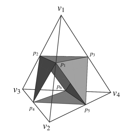
Figure 1: The first stage of the regular subdivision: four child tetrahedra and an octahedron. The faces $(p_{1}p_{4}p_{5})$ and $(p_{2}p_{4}p_{6})$ are transparent.

At every step the most direct approach results in dividing a tetrahedron into eight descendants. The four tetrahedra are obtained by cutting off the corners of the parent tetrahedron at the edge midpoints, as shown on Fig 1. They are obviously similar to their parent. Each of its faces is now composed of the outer faces of three child tetrahedra and one of the faces of an octahedron. The remaining octahedron is split into two pyramids, each of which is separated into two tetrahedra. This splitting depends on the choice of the interior diagonal, so there are three possibilities for this subdivision. In any case, the resulting tetrahedra are not similar to the parent one. There are at least three different similarity classes for the tetrahedra. Moreover, for generic initial tetrahedra a compliance with naturally defined requirements of nestedness, consistency and stability of the subdivisions is not guarantied subtet2 .

We use this scheme only at the last iteration, to produce a four-valent spin network. In all other step w use a different subdivision scheme for octahedra. This refinement rule consists in subdividing an octahedron into six child octahedra and eight tetrahedra by connecting the edge midpoints of each face (Fig. 2(a)) and by connecting all edge midpoints to the barycenter of the parent octahedron (Figs. 2, 3). Even for an arbitrary initial tetrahedron its barycenter

$$b=\frac{1}{4}(v_{1}+v_{2}+v_{3}+v_{4}),$$ (57)

coincides with the barycenter of the child octahedron, which ensures that the eighth second generation tetrahedra are similar to the initial one with the scale factor $1/4=(1/2)^{2}$.

Figure 2: All the octahedron’s edges are divided into equal halves. Connecting the points results in $4\times 8=32$ triangles. On (a) the white triangles are the faces of the second-generation tetrahedra. Each face contributes one tetrahedron, which are shown in (b), inside the outline of the parent octahedron. Each of the octahedron’s vertices contributes a child octahedron. Three of them are shown on (c), where they complete the eight tetrahedron complex to the parent octahedron. of the ch

This similarity can be established either by elementary geometry, using Fig. 3 as an aid, or by finding out the explicit transformation law. As an example, consider the secondary tetrahedron $(bt_{2}t_{3}t_{4})$. Vertices of the initial tetrahedron are mapped into its vertices according to

$$v\mapsto b+\frac{1}{4}v_{1}-\frac{1}{4}v.$$ (58)

Indeed, $v_{1}\mapsto b\equiv b+\frac{1}{4}v_{1}-\frac{1}{4}v_{1}$, and $v_{i}\mapsto t_{i}$.

If at some stage the triangulation consists of $T$ tetrahedra and $O$ octahedra, then one refitment step results in

$$T\mapsto 4T+8O,\qquad O\mapsto T+6O.$$ (59)

Consequently, after $n$ subdivisions

$$T_{n} =\frac{1}{3}\left(2^{3n}+2^{n+1}\right)\sim\frac{2^{3n}}{3},$$ (60)

$$O_{n} =\frac{1}{3}\left(2^{3n-1}-2^{n-1}\right)\sim\frac{2^{3n}}{6}.$$ (61)

Hence the volume fraction of the tetrahedra that are similar to the initial one asymptotically reaches $\frac{1}{3}$. Since the final iteration is followed by a subdivision of the octahedra into four tetrahedra, the $n$ step iterative procedure gives us $T_{n}$ tetrahedra that are similar to the original one (and their volume fraction asymptotically reaches $\frac{1}{3}$), and $T^{\prime}_{n}=4O_{n}$ tetrahedra of other classes.

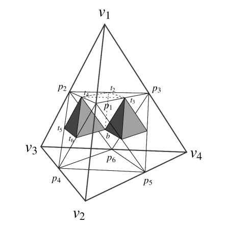
Figure 3: The barycenter $b$ is a common vertex of all the second generation tetrahedra. Two of them are shown as solid bodies, and one as a dotted outline. For a general initial tetrahedron the octahedron’s diagonals $(p_{1}p_{6})$, $(p_{2}p_{5})$, and $(p_{3}p_{4})$ do not intersect at the barycenter.

Assume that the number of steps is such that the surface areas of the small tetrahedra $T$ (and two out of four faces of the tetrahedra $T^{\prime}$) still satisfy $2A_{n}=J_{n}\approx j_{*}\gg 1$. Hence $2A=2^{2n}j_{*}\equiv Kj_{*}$. To establish our point in the simplest possible way we focus only on the tetrahedra $T$. The dimensionality of a (SU(2) invariant) Hilbert space that is associated with a single such tetrahedron is $d_{*}=2j_{*}$, and their total number is $K^{3/2}/3$. The total Hilbert space dimension is

$$d(K)=(2j_{*})^{\frac{1}{3}K^{3/2}}=(2j_{*})^{\frac{1}{3}\left(\frac{2A}{j_{*}}\right)^{3/2}}.$$ (62)

As a result, if the shape is encoded in the information-theoretical optimal way, the shape uncertainty decreases super-exponentially, as

$$\Delta(z_{12})\Delta(z_{23})\propto\frac{1}{d(K)}.$$ (63)

This result ignores the expectation of the volume operator, and its usefulness is mainly in setting the upper limit on the convergence to classicality.

We can use the same construction to show a modest improvement even when the total measured state is given by

$$|\Psi\rangle=\otimes_{a}^{\frac{1}{3}K^{3/2}}|\psi\rangle_{a},$$ (64)

and the state of each $|\psi\rangle$ is given by Eq. (35). If the (commuting!) $J_{12}$ and $J_{23}$ are estimated for all the small tetrahedra independently by separately applying a POVM of Sec. III to each tetrahedron, then the statistical averaging over the entire sample leads to

$$\Delta(z_{12})\Delta(z_{23})\simeq\frac{3c}{2j_{*}}\frac{1}{K^{3/2}},$$ (65)

where a constant $c$ is determined by the asymptotics of a single tetrahedron. As a result, the uncertainty goes to zero faster than the uncertainty of Eq. (34)

VI Conclusions

We constructed a SU(2)-invariant positive operator valued measure that simultaneously extracts two classical parameters that are associated with non-commutative observables. It provides a new method to use SU(2) coherent states to build gauge-invariant objects, thus complementing the analysis of etsi . Mapping the semiclassical problem into a quantum-informational task, we showed that for a single tetrahedron the fuzziness of geometry is reduced only as an inverse of the area. However, a judicious choice of more complicated states speeds-up the convergence. It still remains to be seen weather an exponential convergence to the classical limit is possible.

Appendix A

In elementary quantum measurement theory, a test performed on a finite-dimensional quantum system is represented by a complete set of orthogonal projection operators $\hat{P}_{m}$, where the label $m$ takes at most $d$ different values (d is the dimensionality of the Hilbert space. The probability of obtaining outcome $m$ of that test, following the preparation of a quantum ensemble in a state $\rho$, is

$$p_{m}(\rho)=\operatorname{tr}\rho\hat{P}_{m}.$$

In the infinite-dimensional case such as, e.g., the space of a single one-dimensional non-relativistic particle, the measurement outcomes are associated with spectral decomposition of self-adjoint operators. For example a projection-valued measure for finding a particle in the segment $(a,b)\in\mathbbm{R}$ is written in the improper position basis $|x\rangle$ as

$$\hat{P}((a,b))=\int_{a}^{b}dx|x\rangle\langle x|.$$ (66)

It is well known that this framework is not suitable for description of joint measurements of non-commuting observables, such as non-relativistic position and momentum. Tests of this type are not optimal for many quantum-informational tasks. Moreover, measurement of certain classical quantities (phase, time, relativistic spacetime localization) cannot be described at all in this language.

Those difficulties are overcome with the help of generalized measurements which are described by positive operator-valued measures (POVM). Those are essentially non-orthogonal decompositions of identity by positive operators. Unlike the standard (von Neumann, or projective) measurement descriptions they do not provide a spectral decomposition of some self-adjoint “observable”, while the rest of the rules are kept intact. E.g.,a finite set of outcomes $\mu$ is associated with positive operators $\hat{E}_{\mu}$ that satisfy

$$p_{\mu}(\rho)=\operatorname{tr}(\rho\hat{E}_{\mu}),\qquad\sum_{\mu}\hat{E}_{\mu}={\mathbbm{1}},$$ (67)

but there is no requirement of $\hat{E}_{\mu}\hat{E}_{\nu}=\delta_{\mu\nu}E_{\nu}$. In a finite-dimensional setting it allows to consider an arbitrary number of the measurement outcomes. Covariance considerations play an important role in constructing POVMs and finding the optimal protocols for particular quantum-informational tasks. Their theory is well-developed and is one of the cornerstones of quantum information theory.

We have to keep in mind two related features. First, compared to a corresponding projective measurement, a generalized measurement is less sharp. For example, a Heisenberg uncertainty relation reads $\Delta q\Delta p\geq\hbar/2$, where statistics is taken over an ensemble of identically prepared systems, with position and momentum measured separately on the half of systems each. The optimal POVM for a joint position and momentum measurement results in $\Delta q\Delta p\geq\hbar$ Second, statistical moments in a projective measurement

$$\hat{M}^{(1)}=\sum_{m}x_{m}\hat{P}_{m},\qquad\hat{M}^{(2)}=\sum_{m}x_{m}^{2}\hat{P}_{m},\qquad\ldots$$ (68)

have simple relations with each other, such as

$$\hat{M}^{(2)}=(\hat{M}^{(1)})^{2}.$$ (69)

This is not true for the statistical moments derived from a POVM.

A detailed exposition of POVM theory can be found, e.g., in hol ; bgl ; rmp .

Appendix B

In this Appendix we gather the explicit formulas for the matrix elements of the first two statistical operators of the POVM of Sec. IV. After the angle integration the first moment operator $\hat{M}^{\!(1)}$ of Eq. (47) becomes

$$\hat{M}^{\!(1)}=\sum_{m_{1},m_{2}}m_{1}m_{2}|m_{1}m_{2}\rangle\langle m_{1}m_{2}|+$$

$$\frac{1}{2}\left(\sum_{m_{1}=-j}^{j-1}\sum_{m_{2}=-j+1}^{j}f(m_{1},m_{2})|m_{1}m_{2}\rangle\langle m_{1}+1m_{2}-1|+\sum_{m_{1}=-j+1}^{j}\sum_{m_{2}=-j}^{j-1}f(m_{2},m_{1})|m_{1}m_{2}\rangle\langle m_{1}-1m_{2}+1|\right),$$ (70)

where

$$f(m_{1},m_{2})=\sqrt{(j-m_{1})(j+m_{2})(j+m_{1}+1)(j-m_{2}+1)}.$$ (71)

The second moment operator has a tri-diagonal form,

$$\hat{M}^{\!(2)}=A+B+C$$ (72)

where

$$A=\frac{1}{(2j+3)^{2}}\sum_{m_{1}m_{2}}\left((j+2m_{1}^{2}+1)(j+2m_{2}^{2}+1)+2[(j+1)^{2}-m_{1}^{2}][(j+1)^{2}-m_{2}^{2}]\right)(|m_{1}m_{2}\rangle\langle m_{1}m_{2}|$$ (73)

$$B=\sum_{m_{1}m_{2}}B(m_{1},m_{2})|m_{1}m_{2}\rangle\langle m_{1}+1m_{2}-1|+B({m_{2},m_{1}})|m_{1}m_{2}\rangle\langle m_{1}-1m_{2}+1|,$$ (74)

where

$$B(m_{1},m_{2})=(2m_{1}+1)(2m_{2}-1)\sqrt{(j-m_{1})(j+m_{2})(j+m_{1})(j-m_{2}+1)},$$ (75)

and, finally,

$$C=\sum_{m_{1}m_{2}}C(m_{1},m_{2})|m_{1}m_{2}\rangle\langle m_{1}+2m_{2}-2|+C({m_{2},m_{1}})|m_{1}m_{2}\rangle\langle m_{1}-2m_{2}+2|,$$ (76)

where

$$C(m_{1},m_{2})=\sqrt{(j+m_{2})(j+m_{2}-1)(j-m_{2}+1)(j-m_{2}+2)(j-m_{1})(j-m_{1}-1)(j+m_{1}+1)(j+m_{1}+m_{2})}$$ (77)

Expressions for these operators in $|l,m\rangle$ basis with the help of usual SU(2) recoupling relations. Since the moment operators result from a POVM,

$$\hat{M}^{(2)}\neq(\hat{M}^{(1)})^{2}.$$ (78)

References

- (1) C. Rovelli, Quantum Gravity (Cambridge University Press, Cambridge, 2004); T.Thiemann, Modern Canoninical Quantum General Relativity (Cambridge University Press, Cambridge, 2007).
- (2) B. Dittrich and T. Thiemann, arXiv:0708.1721; C. Rovelli, arXiv:0708.2481.
- (3) A. Barbieri, Nucl. Phys. B 518, 714 (1998); J. C. Baez and J. W. Barrett, Adv. Theor. Math. Phys. 3, 815 (1999).
- (4) C. Rovelli and S. Speziale, Class. Quant. Grav. 23, 5861 (2006).
- (5) E. Bianchi, L. Modesto, C. Rovelli, and S. Speziale Class. Quant. Grav. 23, 6989 (2006).
- (6) E. R. Livine and S. Speziale, arXiv:0711.2455.
- (7) F. Jackson and E. M. Weisstein, Tetrahedron, http://mathworld.wolfram.com/Tetrahedron.html; H. S. M. Coxeter, Regular Polytopes (Macmillan, NY, 1963).
- (8) A. Ashtekar and J. Lewandowski, J. Geom. Phys. 17, 191 (1995).
- (9) A. S. Holevo, Probabilistic and Stattistical Aspects of Quantum Theory (North-Holland, Amsterdam, 1982); A. S. Holevo, Statistical Structure of Quantum Theory (Springer, Berlin, 2001).
- (10) P. M. Busch, M. Grabowski, and P. J. Lahti, Operational Quantum Physics (Springer, Berlin, 1995).
- (11) E. Bagan, M. Baig, A. Brey, R. Muñoz-Tapia, R. Tarrach, Phys. Rev. Lett. 85 5230 (2000); S. D. Bartlett, T. Rudolph, and R. W Spekkens, Rev. Mod. Phys. 79, 555 (2007); N. H. Lindner, A. Peres and D. R. Terno, Phys. Rev. A 68, 042308 (2003).
- (12) A. Peres and D. R. Terno, Rev. Mod. Phys. 76, 93 (2004).
- (13) G. Greiner and R. Grosso, The Visual Computer 16, 357 (2000).
- (14) S. Schaefer, J. Hakenberg, and J. Warren, in Eurographics Symposium on Geometry Processing, p. 151 (2004).