UMN-TH-2704/08 ,     FTPI-MINN-08/25 ,    SLAC-PUB-13372

8-15/08

On Yang–Mills Theories with Chiral Matter

at Strong Coupling

M. Shifman^a,b and Mithat Ünsal ^c,d

^a William I. Fine Theoretical Physics Institute,

University of Minnesota, Minneapolis, MN 55455, USA

^b Laboratoire de Physique Théorique Université de Paris-Sud XI
Bâtiment 210, F-91405 Orsay Cédex, FRANCE

^c SLAC, Stanford University, Menlo Park, CA 94025, USA

^d Physics Department, Stanford University, Stanford, CA 94305, USA

Strong coupling dynamics of Yang–Mills theories with chiral fermion content remained largely elusive despite much effort over the years. In this work, we propose a dynamical framework in which we can address non-perturbative properties of chiral, non-supersymmetric gauge theories, in particular, chiral quiver theories on $S_{1}\times R_{3}$. Double-trace deformations are used to stabilize the center-symmetric vacuum. This allows one to smoothly connect small-$r(S_{1})$ to large-$r(S_{1})$ physics ($R_{4}$ is the limiting case) where the double-trace deformations are switched off. In particular, occurrence of the mass gap in the gauge sector and linear confinement due to bions are analytically demonstrated. We find the pattern of the chiral symmetry realization which depends on the structure of the ring operators, a novel class of topological excitations.

The deformed chiral theory, unlike the undeformed one, satisfies volume independence down to arbitrarily small volumes (a working Eguchi–Kawai reduction) in the large $N$ limit. This equivalence, may open new perspectives on strong coupling chiral gauge theories on $R_{4}$.

1 Introduction

Recent advances in strongly coupled Yang–Mills theories, both analytic and numerical, are quite spectacular. At the same time, our knowledge of (anomaly free) Yang–Mills theories with chiral matter remains at a rudimentary level. All existing methods of exploration fail in the chiral case. Lattice techniques at the moment do not lead to a manifestly gauge invariant formulation of the non-Abelian chiral gauge theories. (For progress in this direction, see [2, 3, 35, 5] and references therein.) Even if a satisfactory gauge invariant lattice formulation was constructed, the well known problem of complex fermion determinants would render numerical simulations impractical. Analytic arsenals of theorists dealing with chiral matter at strong coupling are poor, to put it mildly. The ’t Hooft matching [6] is a useful tool, generally speaking. However, since we will mostly focus on $Z_{K}$-orbifold theories with no continuous global axial symmetries, the ’t Hooft matching [6] is not applicable in this case. AdS/QCD modeling and string theory techniques (so far) do not provide insights into the strong coupling chiral dynamics either.

In essence, the only fact which can be considered established is the perturbative equivalence of the $Z_{K}$ orbifold theories at large $N$ to supersymmetric SU$(KN)$ Yang–Mills theory, with an appropriate rescaling of the gauge couplings [7]. This equivalence does not extend beyond perturbation theory in the chiral case $(K\geq 3)$ due to spontaneous breaking of the chiral symmetry in the parent theory [8] (which is used in the projection). Thus, the above planar equivalence tells us nothing about such basic features of the theory as the vacuum degeneracy/nondegeneracy, patterns of the discrete chiral symmetry breaking and so on, let alone the spectrum of composite colorless hadrons.

In this paper we discuss dynamics of non-Abelian gauge theories with chiral fermion sectors at strong coupling applying and developing ideas suggested in [11]. Our primary target is the so-called $Z_{K}$ orbifold theories at $K\geq 3$. These theories are obtained from supersymmetric SU$(KN)$ Yang–Mills theory by $Z_{K}$ orbifold projection. The gauge group is [SU$(N)]^{K}$, i.e they contain $K$ gluon sectors which are connected to each other only through bifundamental Weyl fermions of the type $\psi_{J}\sim(1,\ldots,N_{J},\overline{N}_{J+1},\ldots 1)$ which transform in the fundamental representation of gauge factor SU$(N)_{J}$ and anti-fundamental of SU$(N)_{J+1}$. Here $J=1,2,...,K$ labels the gauge factors. These theories are also known as “quiver.”

If $K\geq 3$ the mass term for fermions cannot be introduced since there are no gauge invariant bifermion operators. Thus, these theories are genuinely chiral. They have no internal anomalies and are well-defined. It is clear that understanding of strong coupling gauge dynamics is impossible without answering the question of their dynamical behavior, of which next-to-nothing is known. Understanding such theories also carries a phenomenological interest. Strongly coupled chiral gauge theories may be relevant for TeV-scale physics, in particular, bearing responsibility for the electro-weak symmetry breaking, and fermion masses.

Our goal is to understand non-perturbative dynamics of chiral gauge theories in the continuum limit in a locally four-dimensional setting. Currently, there exists no controllable dynamical framework which one could use to address non-perturbative aspects of chiral theories. We suggest one. As a matter of fact, the method designed and applied in vector-like gauge theories with one flavor Ref. [11] (see also [14]) and in pure Yang–Mills theory [15] can be adjusted to become an analytical tool in chiral gauge theories.

The above-mentioned method has several key elements. First, instead of considering Yang–Mills theories on $R_{4}$ we compactify one of the dimensions replacing $R_{4}$ by $R_{3}\times S_{1}$. Then we analyze the theory on $R_{3}\times S_{1}$. At small $r(S_{1})$ the theory can be made weakly coupled, with full control over non-perturbative effects. We perform the so-called “double-trace” deformation of the theory in the small-$r(S_{1})$ domain. It is designed in a such a way that the small-$r(S_{1})$ theory becomes continuously connected to the undeformed theory on $R_{4}$. If the deformation was not performed, we would encounter phase transitions on the way from small to large $r(S_{1})$. Physics of these two domains would be different, and studying the theory at small $r(S_{1})$ would not tell us much about the large-$r(S_{1})$ dynamics. With an appropriately chosen deformation we can avoid unwanted phase transitions ensuring qualitative validity of small-$r(S_{1})$ results at large $r(S_{1})$. The deformed theories are labeled by asterisk, such as YM*.

In fact, the role of the double-trace deformation is to stabilize the center symmetry in the small $r(S_{1})$ regime. Although this deformation is essential at small $r(S_{1})$, it can be switched off at large $r(S_{1})$. The fact that at small $r(S_{1})$ the center symmetry is not spontaneously broken guarantees continuity, at least in the sense of Polyakov’s order parameter. Moreover, the theory is at weak coupling at small $r(S_{1})$. Everything is analytically calculable. The theory has a rich non-perturbative sector which can be treated quasiclassically. It is populated by instanton-monopoles of two types (’t Hooft–Polyakov and Kaluza–Klein) and a variety of composite topological objects built of the above instanton-monopoles. Such composites will be referred to as instanton-monopole molecules. Mathematically, these correspond to magnetic or topological flux carrying operators. In the weak coupling regime, a center-symmetric configuration of the (untraced) Polyakov line behaves as an adjoint Higgs field with a non-vanishing expectation value. The non-Abelian gauge symmetry is spontaneously broken; the gauge structure reduces to the maximal Abelian subgroup,

$${\rm SU}(N)\to\left[{\rm U}(1)^{N-1}\right]\,.$$ (1)

The off-diagonal “$W$ bosons” become heavy at small $r(S_{1})$, and play no role in the infrared (IR) dynamics. The diagonal photons remain massless in perturbation theory.

However, non-perturbatively all (dual) photons acquire mass terms through the magnetic monopole-instantons [15] or magnetic bions [11], via the Polyakov mechanism [19]. This results in formation of the flux “tubes” (strings) in two spatial dimensions, guaranteeing linear confinement. In addition, in QCD*-like theories, the instanton-monopoles generate bifermion vertices leading to spontaneous breaking of the discrete chiral symmetry and a vacuum degeneracy. The very same features — linear confinement and spontaneous breaking of the discrete chiral symmetry — are expected in these theories in the decompactification limit $r(S_{1})\to\infty$. Because of this, we argued [11] the transition from small to large $r(S_{1})$ to be smooth in one-flavor theories.  If so, analytical results reliably obtained at small $r(S_{1})$ can be qualitatively extrapolated into the large-$r(S_{1})$ domain.

The same strategy will be applied to chiral fermions, in particular, in $Z_{K}$ orbifolds ($K\geq 3$), in which at small $r(S_{1})$ (i.e. at weak coupling) the gauge symmetry reduces to

$$[{\rm SU}(N)]^{K}\to\left[{\rm U}(1)^{N-1}\right]^{K}\,.$$ (2)

We calculate non-perturbative effects controlled by instanton-monopole molecules (flux operators) and then use these results to describe general features in the decompactification limit, i.e. in chiral Yang–Mills theories at strong coupling. For this construction to be valid it is important that the $Z_{K}$ orbifold theories have no continuous axial global symmetries.

Compared to QCD-like theories, in chiral theories we find surprises. As was mentioned, the monopole-instantons play a major role in small-$r(S_{1})$ Abelian confinement regime [11]. The most surprising finding in the chiral quiver theories is that, despite the gauge symmetry breaking (2) in the small-$r(S_{1})$ regime, the effect of monopole-instantons identically vanishes! If we denote the monopole-instanton action by $S_{0}$,

$$S_{0}=\frac{8\pi^{2}}{N\,g^{2}_{3+1}}\,,$$ (3)

the leading contribution to the non-perturbative dynamics occurs at order $e^{-2S_{0}}$ via the magnetic bions. The leading terms $e^{-S_{0}}$ in the non-perturbative expansion cancels due to averaging over certain global symmetries. There is also a plethora of non-perturbative flux operators appearing in the $e^{-S_{0}}$ expansion, which are neither monopoles nor instantons and some of which are special for chiral theories.

Although our prime focus is the $Z_{K}$ orbifolds with $K\geq 3$, we will briefly consider another class of chiral gauge theories, namely, a single SU$(N)$ gauge group, with a chiral content, such as one Weyl fermion in the two-index antisymmetric (symmetric) representation supplemented by $N-4$ (correspondingly, $N+4)$ Weyl fermions in the antifundamental representation. A well-known example of this type is the SU(5) gauge theory with one chiral fermion in each of two representations: one ${\bf 10}$ and one $\bf{\bar{5}}$.

We also propose a new method of studying dynamics of the chiral gauge theories on $R_{4}$ by using the concept of large-$N$ volume independence, or the Eguchi–Kawai (EK) reduction. Dynamics of any asymptotically free confining gauge theory formulated on $R_{4-d}\times T_{d}$ in the $N=\infty$ limit is independent of the size of the $d$-torus $T_{d}$, as long as the center symmetry is unbroken [20, 21, 22]. Our deformation of the chiral gauge theories indeed stabilizes the center symmetry in the small-$S_{1}$ regime. Hence, in the $N=\infty$ limit, our suggestion provides a fully reduced model for strongly coupled chiral gauge theories.

Reconciliation of the volume independence in the $N=\infty$ limit, (which is the same as the absence of a weak coupling long distance description) and existence of a semiclassically tractable small-$r(S_{1})$ domain is also non-trivial. The domain of validity of our long-distance description is given by

$$LN\Lambda\ll 1\,.$$ (4)

Here

$$L=2\pi\,r(S_{1})$$ (5)

and $\Lambda$ is the strong scale. As $N\rightarrow\infty$, the region of validity of our analysis shrinks to zero in a correlated manner, in accordance with the large-$N$ volume independence.

2 Chiral orbifold gauge theories: generalities

Consider the orbifold gauge theory in four dimensions with the

$${\rm SU}(N)_{1}\times{\rm SU}(N)_{2}\times\ldots\times{\rm SU}(N)_{K}$$

gauge group, and one bifundamental Weyl fermion on each link,

$$\psi_{J}\sim(1,\ldots,N_{J},\overline{N}_{J+1},\ldots 1),\qquad J=1,\ldots K,\;\;K+1\equiv 1\,.$$ (6)

The matter content of these theories is encoded in a quiver diagram shown in Fig. 1. The action of the theory defined on $R_{3}\times S_{1}$ is given by

$$S=\sum_{J=1}^{K}\int_{R_{3}\times S_{1}}\frac{1}{g^{2}}\,{\rm Tr}\,\left[\frac{1}{2}F_{J,MN}^{2}(x)+i\bar{\psi}_{J}\bar{\sigma}_{M}D_{M}\psi_{J}\right]\,,$$ (7)

where the covariant derivative acts in the bifundamental representation,

$$D_{M}\psi_{J}=\partial_{M}\psi_{J}+iA_{J,M}\psi_{J}-i\psi_{J}A_{J+1,M}\,.$$ (8)

The theory is chiral for $K\geq 3$. For $K\leq 2$ it is vector-like. The $K=1$ theory is in fact ${\mathcal{N}}=1$ super-Yang–Mills (SYM), and the $K=2$ case is the ${\rm SU}(N)\times{\rm SU}(N)$ theory with a single bifundamental representation fermion, which is usually referred to as QCD(BF).

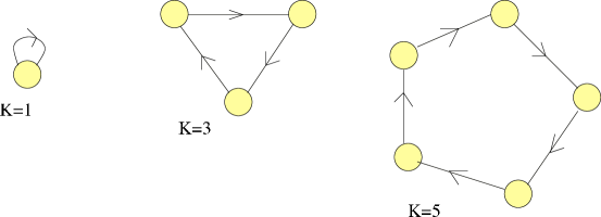
Figure 1: Orbifold gauge theories with odd number of nodes. Nodes represents SU$(N)$ gauge group factors, and arrows are Weyl fermions. The $K=1$ is ${\mathcal{N}}=1$ SYM theory and is vector-like. $K\geq 3$ are chiral since no gauge invariant mass term can be added to the Lagrangian.

Classically, the theory possesses $[{\rm U}(1)]^{K}\times(Z_{K})$ global symmetry acting on elementary fields as

$$[{\rm U}(1)]_{J}:\;\;\psi_{I}\rightarrow e^{i\alpha_{J}\delta_{IJ}}\psi_{I},\;\;$$

$$(Z_{K}):\;\;\;\;\;\psi_{J}\rightarrow\psi_{J+1},\;\;A_{M,J}\ \rightarrow A_{M,J+1}\,.$$ (9)

where $Z_{K}$ is the shift symmetry of the quiver, and the $[{\rm U}(1)]_{J}$ is the (chiral) rotation associated with the fermion $\psi_{J}$. However, quantum mechanically, the current associated with the chiral symmetry is not conserved. Its divergence is

$$\partial_{M}{\mathcal{J}}_{J,M}=\partial_{M}(\bar{\psi}_{J}\bar{\sigma}_{M}\psi_{J})=\frac{N}{16\pi^{2}}\left(F_{J}\widetilde{F}_{J}+F_{J+1}\widetilde{F}_{J+1}\right)$$ (10)

For $K=2$, which is a vector-like theory, we have

$$\partial_{M}(\bar{\psi}_{1}\bar{\sigma}_{M}\psi_{1})=\partial_{M}(\bar{\psi}_{2}\bar{\sigma}_{M}\psi_{2})\,.$$

Thus, the U$(1)_{V}$ current ${\mathcal{J}}_{1}-{\mathcal{J}}_{2}$ is conserved. In the chiral theories with odd $K$, there is no combination of currents which remains conserved. For even $K$, the combination

$${\mathcal{J}}_{M}^{c}\equiv\sum_{J=1}^{K}(-1)^{J}\,{\mathcal{J}}_{J,M}$$

is conserved, $\partial_{M}\,{\mathcal{J}}_{M}^{c}=0$. Hence a global U$(1)$ remains symmetry of the theory for any even $K$.

By the Atiyah–Singer index theorem, the instanton lying in the $J$-th gauge factor has $2N$ fermion zero mode insertions. $N$ of those come from $\psi_{J-1}$ and the other $N$ are due to $\psi_{J}$. The instanton-induced fermion vertex was found by ’t Hooft [23]. The instanton associated with the gauge factor SU$(N)_{J}$ gives

$$I_{J}(x) = e^{-S_{J,\rm inst}}\Big{(}\epsilon_{i_{1},\ldots,i_{N}}(\psi_{J-1})^{i_{1}}_{a_{1}}\ldots(\psi_{J-1})^{i_{N}}_{a_{N}}\Big{)}\Big{(}\epsilon^{k_{1},\ldots,k_{N}}(\psi_{J})_{k_{1}}^{a_{1}}\ldots(\psi_{J})_{k_{N}}^{a_{N}}\Big{)}$$ (11)

$$\sim e^{-S_{J,\rm inst}}\det_{i,k}\left[(\psi_{J-1}\psi_{J})^{i}_{k}\right]=e^{-S_{J,\rm inst}}\det\left[\psi_{J-1}\;\psi_{J}\right]\,,$$

where

$$S_{J,\rm inst}=N\,S_{0}$$ (12)

for all $J$. In the expression $(\psi_{J-1}\psi_{J})^{i}_{k}$, the contracted color indices associated with the gauge group SU$(N)_{J}$ are suppressed. The indices $(i,k)$ belong to SU$(N)_{J-1}\times$ SU$(N)_{J+1}$ gauge factors, the first nearest neighbors of the SU$(N)_{J}$ on the quiver. The determinant (or anti-symmetrization) produces color-singlet instanton operators. We would like to stress that the corresponding weight factor is exponentially small, see Eq. (12).

Since the fermion on the link $J$ communicates with instantons in two gauge groups on which it ends, instanton effects are collective. Regardless of the value of $K$, but depending on whether it is even or odd, the classical symmetry reduces quantum mechanically. From Eq. (11) it is obvious that the symmetry is

$${\rm U}(1)^{K}\rightarrow[Z_{2N}],\qquad\qquad\qquad K{\rm\;odd}\,,$$

$${\rm U}(1)^{K}\rightarrow[Z_{2N}]\times{\rm U}(1),\qquad K\equiv 2m{\rm\;even}\,.$$ (13)

Note that the axial symmetry for all odd-$K$ theories reduces to that of ${\mathcal{N}}=1$ SYM theory while even-$K$ theories have the global symmetry of QCD(BF).

The action of quantum symmetries on the elementary fields is as follows:

$$[Z_{2N}]:\;\;\psi_{I}\rightarrow e^{i\frac{2\pi\,k}{2N}}\psi_{I},\qquad k=1,2,...,2N\,,$$

$$(Z_{K}):\;\;\;\;\;\psi_{J}\rightarrow\psi_{J+1},\;\;A_{M,J}\ \rightarrow A_{M,J+1}\,.$$ (14)

In the chiral quiver theories, no gauge invariant mass term (or gauge invariant local fermion bilinear condensate) is possible.

Local gauge invariant operators that are relevant and will be discussed below are

$$B_{J}(x)=\epsilon_{i_{1},\ldots,i_{N}}\epsilon^{k_{1},\ldots,k_{N}}(\psi_{J})^{i_{1}}_{k_{1}}\ldots(\psi_{J})^{i_{N}}_{k_{N}}\;\equiv\;\det\psi_{J}\,,$$ (15)

and

$$R^{\rm even}(x)\!\! = \!\!(\psi_{1})^{i_{1}}_{i_{2}}\;(\psi_{2})^{i_{2}}_{i_{3}}\;\ldots\;(\psi_{2m})^{i_{2m}}_{i_{1}}\;$$ (16)

$$\equiv {\rm Tr}(\psi_{1}\ldots\psi_{2m}),\qquad\qquad K\equiv 2m\,,$$

$$R^{\rm odd}(x) = (\psi_{1})^{i_{1}}_{i_{2}}\;(\psi_{2})^{i_{2}}_{i_{3}}\;\ldots\;(\psi_{K})^{i_{K}}_{i_{K+1}}(\psi_{1})^{i_{K+1}}_{i_{K+2}}\ldots(\psi_{K})^{i_{2K}}_{i_{1}}$$ (17)

$$\equiv {\rm Tr}(\psi_{1}\ldots\psi_{K}\psi_{1}\ldots\psi_{K}),\;\qquad\qquad K\;{\rm odd}\,.$$

The operator $B_{J}(x)$ in Eq. (15) can be called baryonic and assigned the baryon number $B=1$. The operators $R^{\rm even}$ and $R^{\rm odd}$ in Eqs. (16) and (17) can be called ring and double-ring operators, respectively. The baryon operator is singlet with respect to the axial $[Z_{2N}]\times(-1)^{B}$. Thus, it plays no role in describing the breaking patterns of the chiral $[Z_{2N}]$ symmetry. On the other hand, the chiral ring operators transform as

$$[Z_{2N}]:\,\,\,R^{\rm even}(x)\rightarrow e^{i\frac{2\pi\,m}{N}}R^{\rm even}(x)\,,$$

$$[Z_{2N}]:\,\,\,R^{\rm odd}(x)\rightarrow e^{i\frac{2\pi\,K}{N}}R^{\rm odd}(x)\,.$$ (18)

Thus, they can (and will) be order parameters determining the pattern of the chiral symmetry breaking in the chiral quiver gauge theories. Let us define

$$\widetilde{m}=m\;{\rm mod}\;N,\qquad\widetilde{K}=K\;{\rm mod}\;N\,,$$ (19)

and

$$\gamma(N,\widetilde{m})$$ (20)

denoting the greatest common divisor (gcd) of $N$ and $\widetilde{m}$. Assuming that the chiral condensates (18) acquire a vacuum expectation value (VEV) we get the following chiral symmetry realizations:

$$\langle R^{\rm even}\rangle\neq 0\Longrightarrow\left[Z_{2N}\right]\rightarrow\left[Z_{2\,\gamma(N,\widetilde{m})}\right]\,,$$ (21)

$$\langle R^{\rm odd}\rangle\neq 0\Longrightarrow\left[Z_{2N}\right]\rightarrow\left[Z_{2\,\gamma(N,\widetilde{K})}\right]\,.$$ (22)

This implies occurrence of

$$\widetilde{N}=\left\{\begin{array}[]{ll}\frac{N}{\gamma(N,\widetilde{m})}\,,\quad\mbox{even $K$}\,,\\[8.53581pt] \frac{N}{\gamma(N,\widetilde{K})}\,,\quad\mbox{odd $K$}\end{array}\right.$$ (25)

isolated vacua. Interestingly, if $K$ and $N$ are co-prime, the theory has a maximal chiral symmetry breaking and $N$ isolated vacua. If $N=K$, the theory has a unique vacuum. In general, depending on the relation between $N$ and $K$, the number of vacua $\widetilde{N}$ in this class of theories varies between a unique vacuum and $N$ isolated vacua. The above result disagrees with the statement of Ref. [10] asserting the number of vacua to be $N$ regardless of the relation between $N$ and $K$.

2.1 Collective chirality

For chiral gauge theories to be consistent internal triangle anomalies (Fig. 2) must cancel. The textbook example is SU(5) theory with two Weyl fermions, one in the representations 10 and another in $\overline{\bf 5}$.

Figure 2: Internal chiral anomaly which must cancel after one sums over all fermion species in the triangle loop.

Unlike this old example of consistent chiral gauge theory, in the chiral quiver theories with $K\geq 3$ cancellation of the triangle anomaly proceeds in a collective manner. If all gluons in Fig. 2 belong to one and the same gauge factor $[{\rm SU}(N)]_{J}$, the anomaly cancellation proceeds just like in vector-like theories since at each $J$ we have $N$ fundamental left-handed fermions, and $N$ antifundamental. The triangle diagram trivially vanishes if gluons belong to two (or three) distinct gauge factors.

One can ascribe anomaly coefficients to bifundamental fermions residing on link $J$,

$$(d_{\psi_{J}})_{J^{\prime}}=\delta_{JJ^{\prime}}-\delta_{J+1,J^{\prime}}\,.$$ (26)

Then

$$(d_{\psi_{J-1}}+d_{\psi_{J}})_{J^{\prime}}=\delta_{J-1,J^{\prime}}-\delta_{J+1,J^{\prime}}\,.$$ (27)

Using Eq. (27) we mimic, for each $J$, cancellation of chiral contributions in the triangle graph of Fig. 2 inherent to vector-like theories. Note that although $(d_{\psi_{J-1}}+d_{\psi_{J}})_{J}=0$, the combination $(d_{\psi_{J-1}}+d_{\psi_{J}})_{J\pm 1}=\pm 1$, exhibiting a collective chiral nature of the quiver theory $[{\rm SU}(N)]^{K}$. The anomaly free nature of the latter follows from

$$\sum_{J=1}^{K}\;d_{\psi_{J}}\;=0\,.$$ (28)

It is instructive to compare this collective chirality with a more conventional structure of “old” chiral gauge theories. For example, in the $SU(N)$ gauge theory with one anti-symmetric (AS) representation and $(N-4)$ anti-fundamental $(\overline{\rm F})$ representations, we have $d_{AS}=N-4,\;d_{F}=+1$. Consequently,

$$d_{AS}+(N-4)d_{\overline{F}}=0\,.$$ (29)

2.2 Center symmetry and its stabilization

In [11] and [15] the center stabilizing double-trace deformations were applied to the Yang–Mills theory and QCD-like theories with a massless one-index and two-index representation fermion to control non-perturbative aspects of these theories. In non-Abelian vector-like gauge theories without continuous global symmetries, physics at small $r(S_{1})$ can be smoothly connected with that of the large-$r(S_{1})$ theory ($R_{4}$ theory in the limiting case) by invoking such deformations. In chiral quiver theories we are certain that the small-$r(S_{1})$ and large-$r(S_{1})$ regimes will be indistinguishable by conventional order parameters within the Landau–Ginzburg–Wilson paradigm. Hence, we can use the same strategy as in [11]: at small $r(S_{1})$ quasiclassical computations are possible and reliable. Raison d’être of double-trace deformations is stabilization of the center symmetry at small $r(S_{1})$. Then qualitative lessons about the existence of a mass gap, chiral condensates, chiral symmetry realizations, etc. will continue to hold at large $r(S_{1})$ and on $R_{4}$.

Let us first discuss the center symmetry ${\mathcal{G}}_{C}$ of the chiral quiver theories. The gauge theory compactified on $R_{3}\times S_{1}$ has a global symmetry, which may be identified with aperiodic gauge rotations. In the absence of fermions, we have a decoupled ${\rm SU}(N)^{K}$ gauge group, with a center $[Z_{N}]^{K}$, where each $Z_{N}$ factor is the center group of associated ${\rm SU}(N)$ group. Since the fermions are in the bifundamental representation, they are charged under the consecutive center group factors. For example, the fermion associated with link $J$ carries charge

$$Q_{\psi_{J}}=(0,\ldots,(+1)_{J},(-1)_{J+1},0,\ldots,0)$$ (30)

under the center group $[Z_{N}]^{K}$, where each entry is defined modulo $N$.

Consider an external object charged as $(q_{1},\ldots,q_{N})\in[Z_{N}]^{K}$. It is easy to show that any such $N$-vector can be expressed as

$$(q_{1},\ldots,q_{N})=a_{0}(1,1,\ldots,1)+\sum_{J=1}^{K}a_{J}Q_{\psi_{J}}\,.$$ (31)

The external probe quarks with any linear combinations of charges $Q_{\psi_{J}}$ can be screened by dynamical fermions. However, the multiples of $(1,1,\ldots,1)$ with $a_{0}\neq 0\;({\rm mod}\;N)$ cannot be screened by dynamical quarks, and thus, can be used as external probes to monitor confinement. The center symmetry of the quiver theory is therefore the quotient group

$${\mathcal{G}}_{C}\sim\frac{[Z_{N}]^{K}}{[Z_{N}]^{K-1}}\sim[Z_{N}]_{C}\,.$$ (32)

This is indeed the center symmetry of pure Yang–Mills (YM) theory, ${\mathcal{N}}=1$ SYM and QCD(BF). The presence of the complex dynamical bifundamental fermions reduces the center group $[Z_{N}]^{K}$ down to the diagonal center symmetry $[Z_{N}]_{C}$.

It is possible to determine the realization of the $(Z_{N})_{C}$ symmetry in the small-$S_{1}$ regime of the chiral quiver theories. A one-loop potential for the holonomies

$$U_{J}({\bf x})=Pe^{i\int_{0}^{L}dx_{4}A_{J,4}({\bf x},x_{4})}$$ (33)

where $P$ denote path ordering, is induced by quantum or thermal fluctuations. A simple calculation within the background field method gives

$$V_{\rm eff}[U_{J}] = \frac{2}{\pi^{2}L^{4}}\sum_{J=1}^{K}\sum_{n=1}^{\infty}\frac{1}{n^{4}}\,\Big{[}-|{\rm Tr}\,U^{n}_{J}|^{2}$$ (34)

$$+ \frac{a_{n}}{2}\left({\rm Tr}\,U^{n}_{J}\;{\rm Tr}\,U^{*\,n}_{J+1}+{\rm Tr}\,U^{*\,n}_{J}\;{\rm Tr}\,U^{n}_{J+1}\right)\Big{]}$$

where $K+1\equiv 1$, $\,a_{n}=(-1)^{n}$ for thermal (anti-periodic) spin connection and $a_{n}=+1$ for periodic spin connection. The contribution of a Weyl fermion to the one-loop effective potential is half of the one of the Dirac spinor on the same background, explaining the appearance of the factor ${\textstyle{\frac{1}{2}}}$ in front of the fermion induced terms.

The above one-loop potential also demonstrates why the global center symmetry of the theory is the one given in (32). The gauge-boson contributions to the potential (34) has a $[Z_{N}]^{K}$ symmetry acting as

$$[Z_{N}]_{J}:\;\;{\rm Tr}U_{J^{\prime}}({\bf x})\rightarrow e^{i\frac{2\pi b_{J}}{N}\delta_{JJ^{\prime}}}\;{\rm Tr}U_{J^{\prime}}({\bf x}),\qquad b_{J}=1,\ldots,N\,,$$ (35)

while the part due to the bifundamental fermions locks the independent phase factors $b_{J}$ into the diagonal ($J$-independent) $b$, namely,

$$[Z_{N}]_{C}:\;\;{\rm Tr}U_{J}({\bf x})\rightarrow e^{i\frac{2\pi b}{N}}\;{\rm Tr}U_{J}({\bf x}),\qquad b=1,\ldots,N\,.$$ (36)

This is equivalent to the quotient construction which leaves only the diagonal $[Z_{N}]_{C}$ as the center symmetry of the theory.

On $S_{1}\times R_{3}$ we can deform the original chiral theory (7) by a center-stabilizing double-trace deformation $P[U_{J}({\bf x})]$. The deformed action is

$$S^{*}=S+\int_{R_{3}\times S_{1}}P[U_{J}({\bf x})]$$ (37)

where

$$P[U_{J}({\bf x})]=A\frac{2}{\pi^{2}L^{4}}\,\sum_{J=1}^{K}\sum_{n=1}^{\left[\frac{N}{2}\right]}\frac{2}{n^{4}}\left|\,{\rm Tr}\,U^{n}_{J}({\bf x})\right|^{2}\,,$$ (38)

In (38), $A$ is an overall parameter of order one,  and ${\left[...\right]}$ denotes the integer part of the argument in the brackets. For sufficiently large $A$, the center symmetry remains unbroken in the vacuum (Sect. 2.3). This implies a spontaneous breaking of the non-Abelian gauge symmetry and weak coupling at small $r(S_{1})$, which, in turn, paves the way to the quasiclassical techniques in the chiral gauge theories.

2.3 Perturbation theory

We assemble together expressions in Eqs. (34) and Eqs. (38) and find the stationary point. The center symmetry stability at weak coupling implies that this stationary point, the vacuum of the deformed theory, is located at

$$-i\,\ln\,\langle\,U_{J}\rangle\equiv L\langle\Phi_{J}\rangle$$

$$={\rm diag}\left(-\frac{2\pi[N/2]}{N},\,\,-\frac{2\pi([N/2]-1)}{N},....,\,\frac{2\pi[N/2]}{N}\right)$$ (39)

modulo $2\pi$. Consequently, in the weak coupling regime, the gauge symmetry is broken,

$$[{\rm SU}(N)]^{K}\longrightarrow[{\rm U}(1)^{N-1}]^{K}$$ (40)

to a rank-preserving maximal Abelian subgroup. In perturbation theory $K(N-1)$ photons remain massless while all off-diagonal gauge fields, “$W$ bosons,” acquire masses in the range $\left[\frac{2\pi}{LN},\frac{2\pi}{L}\right]$. The diagonal components of the bifundamental Weyl fermions

$$(\psi_{J})^{i}_{i}\equiv\psi_{J,i},\qquad J=1,\ldots,K,\;\;i=1,...,N$$

remain massless to all orders in perturbation theory. The off-diagonal fermions and $W$ bosons acquire masses

$$m_{(\psi_{J})^{i}_{k}}=m_{(W_{J})^{i}_{k}}=2\pi\frac{(i-k)\;{\rm mod}\;N}{L},$$

and decouple in the low-energy limit. Similarly, the fluctuation of the eigenvalues acquire masses proportional to $g/L$, and are also unimportant at large distances. The eigenvalue distributions of $\ln U_{J}$ are essentially pinned at the bottom (39) of the combined $V_{\rm eff}[U_{J}]+P[U_{J}]$ potential.

The electric charges of each bifundamental fermion $\psi_{J}$ are characterized by concatenation of two $(N-1)$-dimensional vectors under

$$[{\rm U}(1)^{N-1}]_{J}\times[{\rm U}(1)^{N-1}]_{J+1}$$

and neutral under other gauge group factors. Namely,

$$\mbox{\boldmath$q$}_{\psi_{J,i}}=g\,(0,\ldots,0,\underbrace{+\mbox{\boldmath$H$}_{ii}}_{J},\underbrace{-\mbox{\boldmath$H$}_{ii}}_{J+1},0,\ldots,0)\;\in\;[{\rm U}(1)^{N-1}]^{K}$$ (41)

where

$$g\mbox{\boldmath$H$}_{ii}\equiv g(H_{ii}^{1},\ldots,H_{ii}^{N-1})\in[{\rm U}(1)^{N-1}]_{J}$$ (42)

are the electric charges coupled to the $(N-1)$ photons $A_{J,\mu}^{a}$ ($a=1,\ldots,N-1$), and $H$ are the Cartan generators.

If we define

$$\Psi_{J}\equiv\left[\begin{array}[]{ccc}\psi_{J,1}&&\\ &\ddots&\\ &&\psi_{J,N}\end{array}\right],\qquad G_{J}\equiv\left[\begin{array}[]{ccc}e^{i\xi_{J,1}}&&\\ &\ddots&\\ &&e^{i\xi_{J,N}}\end{array}\right],$$ (43)

where $e^{i\xi_{J,i}}\equiv e^{i\mbox{\boldmath$H$}_{ii}\mbox{\boldmath$\xi$}_{J}}$, then the gauge invariance of the low-energy theory takes the form

$$\Psi_{J}\rightarrow G_{J}\Psi_{J}G_{J+1}^{\dagger},\qquad{\rm or},\;\;\psi_{J,i}\rightarrow e^{i\xi_{J,i}}\psi_{J,i}e^{-i\xi_{J+1,i}}\,.$$ (44)

Note that the gauge symmetry is not $[{\rm U}(1)^{N}]^{K}$, but, rather, $[{\rm U}(1)^{N-1}]^{K}$ as it is reflected in $K$ conditions

$$\sum_{i=1}^{N}\xi_{J,i}(x)=\sum_{i=1}^{N}\mbox{\boldmath$H$}_{ii}\mbox{\boldmath$\xi$}_{J}(x)=0\;,$$ (45)

which follow from $\sum_{i=1}^{N}\mbox{\boldmath$H$}_{ii}=0$. Thus, the low-energy effective Lagrangian in perturbation theory is

$${\mathcal{L}}^{\rm pert\,\,th}=\sum_{J=1}^{K}\;\frac{1}{g_{3}^{2}}\,\Big{[}\sum_{a=1}^{N-1}\,\Big{(}\frac{1}{4}F^{a}_{J,\mu\nu}\Big{)}^{2}$$

$$+\sum_{i=1}^{N}i\bar{\psi}_{J,i}\gamma_{\mu}\Big{(}\partial_{\mu}+i\mbox{\boldmath$H$}_{ii}\mbox{\boldmath$A$}_{J,\mu}-i\mbox{\boldmath$H$}_{ii}\mbox{\boldmath$A$}_{J+1,\mu}\Big{)}\psi_{J,i}\Big{]}\,.$$ (46)

This is an all-orders result in perturbation theory. Some erroneous results that one could deduce from the perturbative analysis are (i) the absence of the mass gap for $[{\rm U}(1)^{N-1}]^{K}$ gauge fields (photons); (ii) enhancement of the discrete $(Z_{N})_{A}$ symmetry to continuous $[{\rm U}(1)]^{N}$ fermion number symmetry (this is the fermion number symmetry from the standpoint of three-dimensional large-distance physics); and (iii) no chiral symmetry breaking and no stable flux tubes.

However, all the above conclusions of the perturbative analysis are incorrect, as it was the case also in the nonchiral theories [11]. The most interesting features, such as a mass gap in the gauge sector, stable flux tubes, discrete chiral symmetry breaking are induced due to non-perturbative effects which are invisible in the perturbative analysis.

All non-perturbative effects listed above arise due to non-perturbative dynamics in the quasiclassical approximation. We will identify and classify non-perturbative effects induced by topologically nontrivial field configurations momentarily. By topologically non-trivial configurations, we do not mean only monopole-instantons (fractional instantons) or instantons. In fact, the former play no role in chiral gauge theories (as opposed to the vector-like theories where they play a key role). Interestingly, there exists a new class of topological excitations. Below we give a brief introduction to such flux operators. After a general characterization, we will return to non-perturbative description of the chiral quiver gauge theories.

3 Flux operators or instanton-monopole molecules

In non-Abelian gauge theories in which gauge symmetry reduces to maximal Abelian subgroup at large distances, as in (1) or (2), there are generically stable topological excitations. These excitations are naturally described in framework of the $e^{-S_{0}}$ expansion where $S_{0}$ is the action of the corresponding quasiclassical field configuration.

Below, we show that the non-perturbative dynamics of the chiral theories on small $S_{1}\times R_{3}$ are quite exotic, and very different from the deformed YM theory [15] and vector-like QCD* theories [11] in the same regime.

Perhaps, the most interesting of all is the vanishing of the monopole-instanton operators in the chiral orbifold theories and in chiral gauge theories in general! This excludes the so-called “monopole mechanism” of confinement in the chiral theories. Despite the absence of the monopole operators, there are other magnetically charged excitations and flux-carrying operators.

The flux operators carry either magnetic or topological charges, or both. In the quiver gauge theories formulated on $R_{3}\times S_{1}$ these charges are

$$\left(\int_{S^{2}}F_{J},\qquad\int_{R_{3}\times S_{1}}\frac{g^{2}}{32\pi^{2}}F_{J}^{a}{\widetilde{F}}_{J}^{a}\right)\,.$$ (47)

Any excitation for which either of these two charges does not vanish is either an elementary or composite topological excitation. They can be classified according to the powers of

$$e^{-S_{0}}\equiv e^{-\frac{8\pi^{2}}{g^{2}N}}\,.$$ (48)

In a typical (quiver) gauge theory at small $r(S_{1})$, some relevant flux operators are

$${\rm monopoles:}\qquad e^{-S_{0}}e^{+i\mbox{\boldmath$\alpha$}_{i}\,\mbox{\boldmath$\sigma$}_{J}}\;{\mathcal{O}}_{1}(\psi)\,,$$

$${\rm bions:}\qquad e^{-2S_{0}}e^{+i(\mbox{\boldmath$\alpha$}_{i}-\mbox{\boldmath$\alpha$}_{i\pm 1})\;\mbox{\boldmath$\sigma$}_{J}}\,,$$

$${\rm BPST{\mbox{-}}instantons:}\qquad e^{-NS_{0}}{\mathcal{O}}_{2}(\psi)\,,$$

$${\rm flux\;(monopole)\;rings:}\qquad e^{-KS_{0}}e^{+i\mbox{\boldmath$\alpha$}_{i}\sum_{J}\mbox{\boldmath$\sigma$}_{J}}{\mathcal{O}}_{3}(\psi)\,,$$ (49)

where ${\mathcal{O}}_{1,2,3}$ are various fermionic structures: ${\mathcal{O}}_{2}$ can be read off from Eq. (11), ${\mathcal{O}}_{1}$ and ${\mathcal{O}}_{3}$ are presented in Eqs. (52) and (55), (56), (LABEL:fluxringo), respectively. A sharp distinction between the above field configurations are in their magnetic and topological quantum numbers (47) whose examples are

$${\rm monopoles:}\qquad\left(\pm\frac{4\pi}{g_{3}}\mbox{\boldmath$\alpha$}_{i}\;,\;\pm\frac{1}{N}\right)\,,$$

$${\rm bions:}\qquad\left(\pm\frac{4\pi}{g_{3}}\left(\mbox{\boldmath$\alpha$}_{i}-\mbox{\boldmath$\alpha$}_{i\pm 1}\right)\;,\;0\right)\,,$$

$${\rm BPST{\mbox{-}}instantons:}\qquad\left(0\;,\;\pm 1\right)\,,$$

$${\rm monopole\;rings:}\qquad\left(\pm\frac{4\pi}{g_{3}}(\mbox{\boldmath$\alpha$}_{i_{1}},\ldots,\mbox{\boldmath$\alpha$}_{i_{K}})\;,\;\pm(\frac{1}{N},\ldots,\frac{1}{N})\right)\,,$$ (50)

where the first number in the parentheses stands for the magnetic number, while the second for the topological number.

The monopole operators is a subclass of the flux operators. In a theory without massless fermions, ${\mathcal{O}}_{1}(\psi)$ reduces to unity. In theories with massless fermions, the monopole operators carry a certain number of fermionic zero modes depending on its Callias index [27]. This determines the form of the ${\mathcal{O}}_{1}(\psi)$ operator.

The BPST-intantons [28] carry no magnetic flux, just a net topological charge. The instanton generates certain number of the fermion zero modes dictated by the Atiyah–Singer index theorem. At small $r(S_{1})$ the Callias index theorem carries more refined data than the Atiyah–Singer theorem. As was throughly discussed in [11], in a certain sense the BPST instanton can be viewed as a composite of $N$ types of elementary monopoles. The sum of the Callias indices of “constituent” monopoles is equal to the Atiyah–Singer index, and the product of the monopole operators produces the BPST-instanton vertex. Both topological excitations are well known.

On the other hand, the existence and role of the magnetic bions – topological excitations which carry a magnetic flux, but have no Callias index, and hence, no fermion zero modes – was realized quite recently. They are responsible for the mass gap and confinement in a large class of the QCD-like gauge theories at small $r(S_{1})$ [11]. We will show that the magnetic bions also appear in the chiral gauge theories, and generate a mass gap in the gauge sector.

In the chiral gauge theories there is a new and very interesting class of flux operators carrying both the magnetic flux and fermion zero mode insertions. In fact, they determine the chiral symmetry realization. The structure of these operators is rather unique and special to the chiral theory of interest. We will refer to them as monopole ring operators. They are not limited to the quiver gauge theories and exist virtually in any chiral gauge theory, for instance, in those discussed in Sect. 4. The dynamical role of the monopole ring operators in the issue of the chiral symmetry is similar to that of monopoles (“fractional instantons”) in ${\mathcal{N}}=1$ SYM theory and QCD(AS/S/BF)* theories.

It is desirable to give a fuller classification of the flux operators in both vector-like and chiral gauge theories. Here, we introduce only the flux operators which will capture the leading non-perturbative physics of these theories in the $e^{-S_{0}}$ expansion.

Below, we will discuss non-perturbative dynamics of the chiral quiver theories. Since there are some noteworthy differences between the $K$-even and $K$-odd cases, we examine them separately.

3.1 $K$-even chiral orbifolds ($K=2m$)

In the chiral quiver gauge theories, there are very severe restrictions on the form of the flux operators. To explain the point, let us start from the simplest case, a decoupled pure $[{\rm SU}(N)]^{K}$ gauge theory at small $r(S_{1})$. The presence of the double-trace deformations leads to the gauge symmetry breaking, $[{\rm SU}(N)]^{K}\to[{\rm U}(1)^{N-1}]^{K}$. In this theory a set of disentangled monopole operators emerges,

$$e^{+i\mbox{\boldmath$\alpha$}_{i}\,\mbox{\boldmath$\sigma$}_{J}},\qquad i=1,\ldots N,\qquad J=1,\ldots K\,,$$ (51)

where $\mbox{\boldmath$\sigma$}_{J}$ is the dual photon associated with gauge group [U(1)${}^{N-1}]_{J}$, and $\frac{4\pi}{g}\mbox{\boldmath$\alpha$}_{i}$ is the magnetic charge of the monopole. Each monopole has four bosonic zero modes, three associated with the center of mass position of the monopole ${\bf x}\in R_{3}$ and a U(1) angle associated with the global part of the gauge rotations.

In the presence of massless bifundamental Weyl fermions, there must be two fermion zero modes associated with each monopole. Naively, one expects

$${\mathcal{M}}_{J,i}=e^{-S_{0}}e^{+i\mbox{\boldmath$\alpha$}_{i}\,\mbox{\boldmath$\sigma$}_{J}}\left({\psi_{J-1,i}\;\psi_{J,i}+\psi_{J-1,i+1}\;\psi_{J,i+1}}\right)\,,$$ (52)

as a consequence of the Callias index theorem. From the point of view of the $J$-th gauge group factor, there is nothing wrong with this operator. However, in the chiral quiver theories, the monopole operator at the quiver site $J$ also transforms non-trivially under the global gauge rotations of the nearest-neighbor ($J\pm 1$) sites. For example,

$$\left(\psi_{J-1,i}\psi_{J,i}\right)\rightarrow e^{i\phi_{J-1,i}}\left(\psi_{J-1,i}\psi_{J,i}\right)e^{-i\phi_{J+1,i}}\,,$$ (53)

where $e^{i\phi_{J\pm 1,i}}$ is a global phase. This is the global part of the gauge rotations $e^{i\xi_{J,i}({\bf x})}$ given in Eq. (44). In order to construct a manifestly global-rotation-invariant monopole operator, we have to average over all distinct U$(1)$ angles. The integral $\int d\phi_{J,i}\prod_{J^{\prime}\neq J\pm 1}d\phi_{J^{\prime},i}$ is trivial and produces only an overall numerical factor. For the quiver gauge theories with $K\geq 3$ averaging over the global zero modes of the monopole on the nearest neighbor quiver sites yields

$$\!\!\int d\phi_{J-1,i}d\phi_{J+1,i}\;e^{i\phi_{J-1,i}}\Big{[}e^{-S_{0}}e^{+i\mbox{\boldmath$\alpha$}_{i}\,\mbox{\boldmath$\sigma$}_{J}}\left(\psi_{J-1,i}\psi_{J,i}\right)\Big{]}_{\phi_{J\pm 1}=0}e^{-i\phi_{J+1,i}}\;=\;0$$ (54)

due to either of the integrations, $\int d\phi_{J-1,i}$ or $\int d\phi_{J+1,i}$. Thus, the monopole operators vanish!

Note, however, that the above integral does not vanish for $K=1$, which is ${\mathcal{N}}=1$ SYM theory and for $K=2$ which is QCD(BF)*. Both of these theories are vector-like, and the monopole contribution to the dynamics is non-vanishing as was observed previously [29, 11].

Let us reiterate our striking conclusion: the monopole operator contributions in non-perturbative dynamics of the chiral quiver gauge theories vanish identically. Upon averaging over all zero modes, in particular, the global U$(1)$ angles, all monopole operators drop out.

The structure of the monopole operators and transformation properties under the global rotations given in Eq. (53) also suggest how to construct flux operators invariant under the the global U$(1)$ symmetries of the theory. If we take the product of the “naive” $K/2=m$ monopole operators (see Eq. (52)) separated by two units in the quiver diagram, the resulting topological excitation will present a gauge invariant flux operator with $K=2m$ fermion insertions. There are two types of the monopole ring operators associated with product of the naive monopole operators on even and odd sublattice of the quiver. For even quiver sublattice these flux operators are

$${\mathcal{M}R}_{i}^{\rm even}(x)= e^{-\frac{KS_{0}}{2}}\Big{(}\prod_{J\in{\rm even}}e^{+i\mbox{\boldmath$\alpha$}_{i}\mbox{\boldmath$\sigma$}_{J}}\Big{)}\left(\psi_{1,i}\ldots\psi_{2m,i}\;+\;\psi_{1,i+1}\ldots\psi_{2m,i+1}\right)$$

$$\equiv e^{-mS_{0}}\Big{(}e^{+i\mbox{\boldmath$\alpha$}_{i}\sum_{J=1}^{m}\mbox{\boldmath$\sigma$}_{2J}}\Big{)}\left(R^{\rm even}_{i}(x)+R^{\rm even}_{i+1}(x)\right),$$ (55)

while for the odd sublattice

$${\mathcal{M}R}_{i}^{\rm odd}(x)= e^{-\frac{KS_{0}}{2}}\Big{(}\prod_{J\in{\rm odd}}e^{+i\mbox{\boldmath$\alpha$}_{i}\mbox{\boldmath$\sigma$}_{J}}\Big{)}\left(\psi_{1,i}\ldots\psi_{2m,i}\;+\;\psi_{1,i+1}\ldots\psi_{2m,i+1}\right)$$

$$\equiv e^{-mS_{0}}\Big{(}e^{+i\mbox{\boldmath$\alpha$}_{i}\sum_{J=1}^{m}\mbox{\boldmath$\sigma$}_{2J-1}}\Big{)}\left(R^{\rm even}_{i}(x)+R^{\rm even}_{i+1}(x)\right),$$ (56)

where $i\in[1,...,N]$.

The fermionic structure of the two flux operators,

$${\mathcal{M}R}_{i}^{\rm even}(x)\,\,\,{\rm and}\,\,\,{\mathcal{M}R}_{i}^{\rm odd}(x)\,,$$

is identical. Clearly, the monopole ring operators are not forbidden by symmetries of the theory and are consistent with natural generalization of the Callias index theorem. Namely, these operators have $K/2=m$ constituent monopoles, and $K=2m$ fermion zero mode insertions. However, as was noted above, the notion of a constituent monopole-instanton is somewhat misleading since such “constituents” do not exist in the isolated state, nor do they contribute to non-perturbative dynamics. In addition to Eqs. (55) and (56), certainly, there are conjugates of these topological excitations, to be labeled as $\overline{\mathcal{M}R}^{\rm odd/even}_{i}(x)$.

We will see that the flux ring operators are responsible for various non-perturbative phenomena, such as the discrete chiral symmetry realization. In particular, note that the chiral order parameter defined in (17) is related to the fermion zero mode structure of the flux operators as follows:

$$R^{\rm even}(x)=\sum_{i=1}^{N}R^{\rm even}_{i}(x)+\;(\rm massive\;modes).$$ (57)

Exotic chiral condensates can be saturated by the flux ring operators, much in the same way as the usual chiral condensates are saturated by the monopole operators at small $r(S_{1})$ in ${\mathcal{N}}=1$ SYM theory and QCD(BF)* [29, 11]. Just like in the ${\mathcal{N}}=1$ theory and QCD(BF)*, the monopole ring operators with the fermion zero mode insertions have nothing to say on the issue of the mass gap and confinement in the chiral gauge theory [11].

3.1.1 Mass gap in the gauge sector

In perturbation theory, a mass term for photon is forbidden. Thus, we are searching for non-perturbative effects that may generate a mass gap in the gauge sector of the theory. Let us first show that mass gaps for the photons are allowed by the symmetries of the microscopic theory.

Since the symmetry of the microscopic theory is ${\rm U}(1)_{V}\times[(Z_{2N})]\times Z_{K}$, it must be manifest in the low-energy effective theory. The invariance of the monopole ring operators (55) and (56) under the $[(Z_{2N})]$ discrete chiral symmetry requires intertwining of the axial chiral symmetry with a discrete shift symmetry of the dual photons,

$$[(Z_{2N})]:\;\;\;\;R_{i}(x) \longrightarrow e^{i\frac{2\pi\widetilde{m}}{N}}R_{i}(x),$$

$$\sum_{J\in{\rm even}}\mbox{\boldmath$\sigma$}_{J} \longrightarrow\sum_{J\in{\rm even}}\mbox{\boldmath$\sigma$}_{J}-\frac{2\pi\widetilde{m}}{N}\mbox{\boldmath$\rho$}\,,$$ (58)

where $\rho$ is the Weyl vector defined by

$$\mbox{\boldmath$\rho$}=\sum_{k=1}^{N-1}\mbox{\boldmath$\mu$}_{k}\,,$$ (59)

and $\mu$_k’s stand for the $N-1$ fundamental weights of the associated Lie algebra, defined through the reciprocity relation,

$$\frac{2\mbox{\boldmath$\alpha$}_{i}\mbox{\boldmath$\mu$}_{j}}{\mbox{\boldmath$\alpha$}_{i}^{2}}=\mbox{\boldmath$\alpha$}_{i}\mbox{\boldmath$\mu$}_{j}=\delta_{ij}\,.$$ (60)

Using the identities

$$\mbox{\boldmath$\alpha$}_{N}\mbox{\boldmath$\rho$}=-(N-1)\,,\quad\mbox{\boldmath$\alpha$}_{i}\mbox{\boldmath$\rho$}=1\,,\quad i=1,\,\ldots\,N-1\;,$$ (61)

we see that the flux operator

$$\left(\prod_{J\in{\rm even}}e^{+i\mbox{\boldmath$\alpha$}_{i}\,\mbox{\boldmath$\sigma$}_{J}}\right)\rightarrow e^{-i\frac{2\pi\widetilde{m}}{N}}\;\left(\prod_{J\in{\rm even}}e^{+i\mbox{\boldmath$\alpha$}_{i}\,\mbox{\boldmath$\sigma$}_{J}}\right)\,,\quad i=1,\,\ldots,\,N\,,$$ (62)

i.e. rotates in the opposite direction compared to the $2m$-linear fermion ring operators $R_{i}(x)$, by the same amount. Hence, the monopole ring vertex (55) is invariant under the discrete $[(Z_{2N})]$ chiral symmetry. Note that the discrete shift symmetry acting on the dual photons is

$$Z_{\widetilde{N}},\qquad{\rm where}\;\;\widetilde{N}=\frac{N}{{\gamma}({\widetilde{m}},N)}\;.$$ (63)

Recall that $\gamma({\widetilde{m}},N)={\rm gcd}({\widetilde{m}},N)$. This discrete shift symmetry, as opposed to the continuous shift symmetries, cannot prohibit mass terms for scalars; at best it can defer the appearance of a mass term to higher levels of the $e^{-S_{0}}$ expansion. Thus, the scalar mass terms will indeed be generated. The flux operators such as $e^{-S_{0}}e^{+i\mbox{\boldmath$\alpha$}_{i}\,\mbox{\boldmath$\sigma$}_{J}}$ are forbidden by the shift symmetry and are not allowed by the index theorem. There are topologically null, but magnetically charged excitations in the theory referred to as the magnetic bions. The magnetic bion operators are

$$e^{-2S_{0}}e^{+i(\mbox{\boldmath$\alpha$}_{i}-\mbox{\boldmath$\alpha$}_{i\pm 1})\,\mbox{\boldmath$\sigma$}_{J}}\,,$$ (64)

which is roughly the product of the monopole and anti-monopole operators, stripped off their fermionic modes. The magnetic bion contribution to the non-perturbative part of the Lagrangian is

$$\Delta{\mathcal{L}}_{\rm bions}=e^{-2S_{0}}\sum_{J=1}^{2m}\sum_{i=1}^{N}\cos{(\mbox{\boldmath$\alpha$}_{i}-\mbox{\boldmath$\alpha$}_{i-1})\,\mbox{\boldmath$\sigma$}_{J}}\,.$$ (65)

This is sufficient to render all photons massive. Defining the Fourier transform of the dual photons as

$${\widetilde{\sigma}}_{J,p}=\frac{1}{\sqrt{N}}\sum_{i^{\prime}=1}^{N}e^{i\frac{2\pi i^{\prime}p}{N}}\mbox{\boldmath$H$}_{i^{\prime}i^{\prime}}\mbox{\boldmath$\sigma$}_{J}$$ (66)

diagonalizes the mass matrix leading to the following masses for the dual photons:

$$m_{{\widetilde{\sigma}}_{J,p}} = e^{-S_{0}}\left(2\sin\frac{\pi p}{N}\right)^{2}$$ (67)

$$= \Lambda(\Lambda LN)^{2}\left(2\sin\frac{\pi p}{N}\right)^{2},\qquad J\in[1,K],\;\;p\in[1,N-1]\,.$$

In the second line we restored dimensions and used the one-loop renormalization group relation $(\Lambda LN)^{3}=e^{-\frac{8\pi^{2}}{g^{2}N}}$. The $J$ independence of this mass formula is an artifact of our truncation of the $e^{-S_{0}}$ expansion at the leading order, $e^{-2S_{0}}$. The $J$-degeneracy will be lifted by subleading terms in the $e^{-S_{0}}$ expansion. For our purposes it is most important that all $(N-1)K$ dual photons of the chiral theory acquire masses at this order.

The effect due to the operators (49) in the large-distance effective Lagrangian is

$${\mathcal{L}}^{\rm effective} = {\mathcal{L}}^{\rm pert\;th}+{\mathcal{L}}^{\rm non\;pert}$$ (68)

$$= {\mathcal{L}}^{\rm pert\;th}+\Delta{\mathcal{L}}_{\rm bions}+\Delta{\mathcal{L}}_{\rm monopole\;ring}+\Delta{\mathcal{L}}_{\rm instantons}+\ldots$$

The physics that this Lagrangian encapsulates is the main result of our work. The flux operators in the large-distance Lagrangian (68) present microscopic sources for various non-perturbative phenomena. The dual photon masses are generated by magnetic bions. Linear confinement ensues much in the same way as in non-chiral theories. The chiral condensates are saturated by the monopole ring operators. Below, we will discuss the chiral condensates in the quiver theories in more detail.

3.1.2 Chiral condensates and chiral symmetry realization

The chiral condensate $\langle{\rm Tr}(\psi_{1}\ldots\psi_{2m})\rangle$ is dominated by a contribution from the flux ring operators (55) and (56). The chiral condensate operator has $2m$ fermion insertions. It is saturated by the zero mode structure of the flux ring operators. This is analogous to ${\mathcal{N}}=1$ SYM theory at small $r(S_{1})$ where the chiral condensate is saturated by the monopole operators with two zero mode insertions [29]. The chiral condensate is proportional to

$$\langle{\rm Tr}(\psi_{1}\ldots\psi_{2m})\rangle \sim \sum_{i=1}^{N}\;\;\langle{\rm Tr}(\psi_{1}\ldots\psi_{2m})\rangle_{{\mathcal{M}R}_{i}^{\rm even/odd}}$$ (69)

$$= 2Ne^{-mS_{0}}e^{i\frac{2\pi m}{N}}\,.$$

Expressing it in terms of the strong scale by using the one-loop result for the $\beta$ function, we obtain

$$\langle\Omega_{q}|{\rm Tr}(\psi_{1}\ldots\psi_{2m})|\Omega_{q}\rangle=2N\Lambda^{3m}e^{i\frac{2\pi q}{\widetilde{N}}},\qquad q=1,\ldots,{\widetilde{N}}\,.$$ (70)

This shows that the chiral symmetry breaking pattern of the theory is the one given in Eq. (21). As was anticipated in (25), the theory possesses ${\widetilde{N}}$ vacua,

$$\left\{|\Omega_{1}\rangle,\ldots,|\Omega_{\widetilde{N}}\rangle\right\},\qquad{\widetilde{N}}=\frac{N}{{\gamma}(N,{\widetilde{m}})}\,.$$ (71)

The phase of the chiral condensate distinguishes these vacua.

We can label the vacua in the $\langle{\rm Tr}(\psi_{1}\ldots\psi_{2m})\rangle$-plane, and study aspects of domain walls of the chiral gauge theory (in cases where there are multiple vacua).

The chiral condensate (70) is an interesting result. It tells us that the condensate is independent of $r(S_{1})$ in the weak coupling regime. Such radius independence occurs in a few QCD-like theories as well. These are ${\mathcal{N}}=1$ SYM and QCD(BF/AS/S)* theories with a single Dirac fermion. In ${\mathcal{N}}=1$ SYM theory the chiral order parameter is a part of the so called chiral ring and is protected by supersymmetry. In QCD(BF/AS/S)* theories the chiral condensate must coincide with that in ${\mathcal{N}}=1$ theory due to planar equivalence [30, 31, 32, 8, 33]. Indeed, the microscopic quasiclassical calculation at small $r(S_{1})$ gives the same result as the $R_{4}$ prediction in the framework of planar orbifold/orientifold equivalences. This suggests that, perhaps, the value of the condensate in the quiver theory under consideration remains invariant under decompactification into $R_{4}$.

3.1.3 Linear confinement

As was discussed in Sect. 2.2, in the $[{\rm SU}(N)]^{K}$ chiral quiver gauge theory with dynamical bifundamental fermions, linear confinement (with unbreakable strings) can be probed by external charges with non-vanishing $N$-ality

$$k(1,1,\ldots,1),\qquad k=1,\ldots,N-1$$ (72)

under the diagonal center group $[Z_{N}]_{C}$. Below we will demonstrate the existence of a linearly confining potential between such probe external charges. The corresponding tensions are determined by the dual photon mass terms generated by the bion operator (65). Precision evaluation of the tensions will not be carried out.

The insertion of a Wilson loop $W_{{\mathcal{R}}}(C)$ in a representation $\mathcal{R}$ with non-zero $N$-ality $k$ corresponds, in the low-energy dual theory, to the requirement that the dual scalar fields have non-trivial monodromy,

$$\int_{C^{\prime}}(d\mbox{\boldmath$\sigma$}_{1},\ldots,d\mbox{\boldmath$\sigma$}_{K})=2\pi(\mbox{\boldmath$\mu$}_{k},\ldots,\mbox{\boldmath$\mu$}_{k})\,,$$ (73)

where $C^{\prime}$ is any closed curve whose linking number $\ell$ with $C$ is one:

$${\ell}\;(C,C^{\prime})=1$$ (74)

regardless of the details of the contour $C^{\prime}$. In other words, in the presence of the Wilson loop $W_{{\mathcal{R}}}(C)$ the dual scalar fields must have a discontinuity of $2\pi\mbox{\boldmath$\mu$}_{k}$ across some surface $\Sigma$ which spans the loop $C$.

To evaluate a Wilson loop expectation value sourced by the charges (72), one must minimize the dual magnetic bion induced action in the space of field configurations satisfying the monodromy condition (73). Adapting Polyakov’s argument to our present problem, we find the string tension

$$T_{k}\equiv-\lim_{\mathrm{area}(\Sigma)\to\infty}\frac{\ln\left\langle W_{\mathcal{R}}(C)\right\rangle}{\mathrm{area}(\Sigma)}\equiv\left.\min_{\mbox{\boldmath$\sigma$}_{J}}\;\frac{\Delta S_{\rm bion}(\mbox{\boldmath$\sigma$}_{J})}{\mathrm{area}({\mathbb{R}}^{2})}\right|_{\Delta(\mbox{\boldmath$\sigma$}_{1},\ldots,\mbox{\boldmath$\sigma$}_{K})}$$ (75)

where

$$\Delta\mbox{\boldmath$\sigma$}_{J}=\mbox{\boldmath$\sigma$}_{J}(\infty)-\mbox{\boldmath$\sigma$}_{J}(-\infty)=\mbox{\boldmath$\mu$}_{k}$$

and $\Delta S_{\rm bion}(\mbox{\boldmath$\sigma$}_{J})$ is the magnetic bion action minus its vacuum value. Note that due to the equivalence relations

$$\mbox{\boldmath$\mu$}_{k}=k\mbox{\boldmath$\mu$}_{1}+\mbox{\boldmath$\alpha$}$$

for some $\alpha$ in the root lattice, we are guaranteed to have $T_{k}=T_{N-k}$ for the string tensions. The $k$-string tension $T_{k}$ equals the mass of a kink solution with topological charge $k$.

The linearly confining chiral quiver gauge theories are similar to pure YM theory or YM theory with adjoint fermions. In both cases, there are $N-1$ types of stable flux tubes associated with an unbroken $Z_{N}$ gauge symmetry in the infrared.

The reader should also note that the monodromy condition (73) is different from the change of the value of the dual photon scalar in passing from one isolated vacuum of the theory to another (in cases where there are multiple vacua). The latter is associated with the spontaneous breaking of the $Z_{\widetilde{N}}$ discrete shift symmetry (or the discrete chiral symmetry) while the ${\widetilde{N}}$ isolated vacua are separated by

$$\Delta\Big{(}\sum_{J\in\rm even}\mbox{\boldmath$\sigma$}_{J}\Big{)}=\frac{2\pi\widetilde{m}}{N}\mbox{\boldmath$\rho$}\,.$$ (76)

In our case, the monodromy is due to an external source probing the vacuum of the theory and the jump across the interface of the Wilson loop is not associated with any spontaneous symmetry breaking. The directions of these two types of monodromies in the field space are not parallel to each other.

3.2 Odd-$K$ chiral orbifolds

Dynamics of the center stabilized odd-$K$ chiral orbifold theories is similar to that of their even-$K$ counterparts. Below, we will only outline the differences.

The gauge invariant flux (monopole) ring operators, the analogs of (55) and (56), are

$${\mathcal{M}R}_{i}(x)= e^{-KS_{0}}\Big{(}\prod_{J}e^{+i\mbox{\boldmath$\alpha$}_{i}\mbox{\boldmath$\sigma$}_{J}}\Big{)}\left(\psi_{1,i}\ldots\psi_{K,i}\psi_{1,i}\ldots\psi_{K,i}\;+[i\rightarrow i+1]\right)$$

$$\equiv e^{-KS_{0}}\Big{(}e^{+i\mbox{\boldmath$\alpha$}_{i}\sum_{J=1}^{K}\mbox{\boldmath$\sigma$}_{J}}\Big{)}\left(R_{i}(x)+R_{i+1}(x)\right),\quad i=1,\ldots,N.$$

As was discussed in Sect. 2, the microscopic theory possesses a $[(Z_{2N})]$ axial symmetry. Hence, this must also be a symmetry of the large-distance effective theory. This is possible due to intertwining of the chiral symmetry with the shift symmetry of the dual photons,

$$[(Z_{2N})]:\;\;\;\;R_{i}(x) \longrightarrow e^{i\frac{2\pi K}{N}}R_{i}(x),$$

$$\sum_{J}\mbox{\boldmath$\sigma$}_{J} \longrightarrow\sum_{J}\mbox{\boldmath$\sigma$}_{J}-\frac{2\pi K}{N}\mbox{\boldmath$\rho$}\,.$$ (78)

The $Z_{2N}$ discrete axial symmetry transmutes into the dual photon as a discrete $Z_{\widetilde{N}}$ symmetry where $\widetilde{N}$ is given in (25). The spontaneous breaking of $Z_{\widetilde{N}}$ is responsible for the existence of $\widetilde{N}$ isolated vacua. As before, if $\widetilde{N}$ is equal to unity, then the $Z_{2N}$ chiral symmetry of the microscopic theory remains unbroken.

The chiral condensate $\langle{\rm Tr}(\psi_{1}\ldots\psi_{K}\psi_{1}\ldots\psi_{K})\rangle$ receives its dominant contribution from the monopole ring operators (LABEL:fluxringo) discussed above. Proceeding along the lines of Sect. (3.1.2), we arrive at

$$\langle\Omega_{q}|{\rm Tr}(\psi_{1}\ldots\psi_{K}\psi_{1}\ldots\psi_{K})|\Omega_{q}\rangle=N\Lambda^{3K}e^{i\frac{2\pi q}{\widetilde{N}}},\qquad q=1,\ldots,{\widetilde{N}}\,.$$ (79)

This formula shows that the pattern of the chiral symmetry breaking of the theory is that presented in Eq. (21). As anticipated in (25), the theory possess ${\widetilde{N}}$ vacua,

$$\left\{|\Omega_{1}\rangle,\ldots,|\Omega_{\widetilde{N}}\rangle\right\},\qquad{\widetilde{N}}=\frac{N}{{\gamma}(N,{\widetilde{K}})}\,.$$ (80)

Other aspects of the odd-$K$ chiral quiver theories are very similar to the even-$K$ case. In particular, the mechanism of the mass gap generation in the gauge sector is the same in both cases, and is due to the magnetic bions.

4 Chiral theories of the second type

In this section, we will briefly discuss the chiral gauge theories of a traditional type, with a single gauge group factor and a chiral matter content. Examples are SU$(N)$ gauge theory with one AS (S) Weyl fermion and $N-4$ $(N+4)$ anti-fundamental representation Weyl fermions. The gauge anomaly coefficient of the AS (S) representation is $N-4$ $(N+4)$ and that of the fundamental representation is $+1$. Hence, these theories are internally free of triangle anomalies, and are self-consistent. Below, we consider the theory with the AS fermions as an example.

Classically, the theory possesses an ${\rm U}(1)_{a}\times{\rm U}(1)_{b}\times{\rm SU}(N-4)$ global symmetry defined by

$${\rm U}(1)_{a}:\quad\psi_{[ab]}\rightarrow e^{i\beta}\psi_{[ab]}\,,$$

$${\rm U}(1)_{b}:\quad\psi^{a}_{I}\rightarrow e^{i\delta}\psi^{a}_{I},\qquad I=1,\ldots N-4\,,$$

$${\rm SU}(N-4):\quad\psi^{a}_{I}\rightarrow(V\psi^{a})_{I},\qquad V\in{\rm SU}(N-4)\,.$$ (81)

In the quantum theory, due to instanton effects, only the ${\rm U}(1)\times{\rm SU}(N-4)$ symmetry survives.

Recall that the BPST instanton has $N-2$ insertion of antisymmetric $\psi_{[ab]}$’s along with $N-4$ antifundamental fermion zero mode insertions, one for each flavor. A manifestly SU$(N-4)$ global symmetry invariant instanton operator is proportional to

$$I_{\rm inst}=e^{-S_{\rm inst}}\underbrace{\psi_{[a_{1}b_{1}]}\ldots\psi_{[a_{N-2}b_{N-2}]}}_{{N-2}}\underbrace{\psi^{b_{1}}_{I_{1}}\ldots\psi^{b_{N-4}}_{I_{N-4}}}_{N-4}\epsilon^{I_{1}\ldots I_{N-4}}\epsilon^{a_{1}\ldots a_{N-2}b_{N-3}b_{N-2}}\,.\\$$

Clearly, the instanton effect spoils one particular linear combination of the classical U$(1)$ symmetries. The linear combination which is preserved by the instanton vertex is

$$e^{i\alpha Q}\psi_{[ab]}=e^{i\alpha(N-4)}\psi_{[ab]},\qquad e^{i\alpha Q}\psi^{a}=e^{-i\alpha(N-2)}\psi^{a}\,.$$ (82)

We consider this gauge theory at small $r(S_{1})$ with either periodic or antiperiodic spin connection. For what follows, the difference is immaterial. The one-loop potential can be obtained as in (34),

$$V_{\rm eff}[U_{J}] =\frac{2}{\pi^{2}L^{4}}\sum_{n=1}^{\infty}\frac{1}{n^{4}}\,\Big{\{}-|{\rm Tr}\,U^{n}|^{2}$$ (83)

$$+\frac{a_{n}}{2}\Big{[}\Big{(}\frac{({\rm Tr}\,U^{n})^{2}-({\rm Tr}\,U^{2n})}{2}+(N-4){\rm Tr}\,U^{n}\Big{)}+{\rm h.c.}\Big{]}\Big{\}}.$$

where the fermionic contributions (the second line) is half of the Dirac fermions in the corresponding representation. Regardless of the spin connection, this potential exhibits attraction between the eigenvalues of the Polyakov line. In the thermal case, the theory will be in the deconfined high temperature phase.

At small $r(S_{1})$ we add a double-trace deformation which generates a repulsion among the eigenvalues of the Polyakov line. As opposed to the chiral quivers where there is an exact $[Z_{N}]_{C}$ center symmetry, the “traditional” chiral SU$(N)$ theory has no exact center symmetry. What our double-trace deformation does in this case, is to provides an eigenvalue repulsion rendering the vacuum as close as possible to the center-symmetric

$$L\langle\Phi\rangle={\rm diag}\left(-\frac{2\pi[N/2]}{N},\,\,-\frac{2\pi([N/2]-1)}{N},....,\,\frac{2\pi[N/2]}{N}\right)\,,$$ (84)

point, i.e., close to the vacuum of the pure YM* theory in the weak coupling regime.

At small $r(S_{1})$, when the gauge coupling is small, the eigenvalue fluctuations around the center stabilized minimum (84) are small. This implies that at large distances the gauge structure reduces to the ${\rm U}(1)^{N-1}$ subgroup of SU$(N)$. Due to the broken gauge symmetry, the perturbative spectrum at low energies reduces to massless photons and massless fermions charged under the ${\rm U}(1)^{N-1}$ gauge group. We want to know whether or not non-perturbative effects destabilize the masslessness of these excitations. More specifically, we want to understand whether or not the gauge fluctuations are gapped. As usual, non-perturbative topological excitations are classified in powers of $e^{-S_{0}}$.

Appropriate analysis runs parallel to that in the chiral quiver theories. It is slightly more technical, however. The differences we will encounter are analogous to those between the vector-like QCD(BF)* theory and QCD(AS)* theories discussed in our earlier work [11]. We recall that QCD(BF)* was technically much simpler due to various implications of the Callias index theorem. In particular, in both QCD(BF)* and QCD(AS)*, there are $N$ monopole operators, but the former has a total of $2N$ zero modes distributed evenly (two for each monopole) between the monopoles. The latter has $2N-4$ zero modes, two for $N-2$ monopoles and nothing for the remaining two. (See Eqs. (75) and (52) in [11] and discussion on page 37 on the relation between the Callias and Atiyah–Singer index theorems.) Also it is worth recalling that for QCD(F)* theory with one fundamental fermion, the BPST instanton has two fermion zero modes. They must be distributed among $N$ monopoles as follows: two fermion insertions attached to one monopole, with no fermion insertions in the remaining $N-1$ monopoles. All these distributions of zero modes are a natural consequence of the Callias index theorem.

Similar to what happens in the chiral quiver theories, in the “traditional” chiral theories $(N-1)$ out of $N$ monopole operators vanish due to averaging over a certain global part of the gauge symmetry. A single monopole operator (which does not carry fermion zero mode insertions) is the only contribution in the $e^{-S_{0}}$ expansion at the level $e^{-S_{0}}$.

Naive monopole operators can be found by truncating various monopole operators in the QCD(AS)* and QCD(F)* theories of Ref. [11]. In a sense, the chiral theory at hand is a combination of QCD(AS)* and $(N-4)$ QCD(F)* stripped off of their chiral partners. The resulting operators are

$${\mathcal{M}}_{1}=e^{-S_{0}}e^{i\mbox{\boldmath$\alpha$}_{1}\mbox{\boldmath$\sigma$}}\;(\lambda_{1}+\lambda_{2})\,,$$

$${\mathcal{M}}_{2}=e^{-S_{0}}e^{i\mbox{\boldmath$\alpha$}_{2}\mbox{\boldmath$\sigma$}}\;(\lambda_{2}+\lambda_{3})\,,$$

$$\ldots\,,$$

$${\mathcal{M}}_{m-1}=e^{-S_{0}}e^{i\mbox{\boldmath$\alpha_{m-1}$}\mbox{\boldmath$\sigma$}}\;(\lambda_{m-1}+\lambda_{m})\,,$$

$${\mathcal{M}}_{m}=e^{-S_{0}}e^{i\mbox{\boldmath$\alpha$}_{m}\mbox{\boldmath$\sigma$}}\;(2\lambda_{m})\,,$$

$${\mathcal{M}}_{m+1}=e^{-S_{0}}e^{i\mbox{\boldmath$\alpha$}_{m+1}\mbox{\boldmath$\sigma$}}\;(\lambda_{m}+\lambda_{m-1})\,,$$

$$\ldots\,,$$

$${\mathcal{M}}_{2m-2}=e^{-S_{0}}e^{i\mbox{\boldmath$\alpha$}_{2m-2}\mbox{\boldmath$\sigma$}}\;(\lambda_{3}+\lambda_{2})\,,$$

$${\mathcal{M}}_{2m-1}=e^{-S_{0}}e^{i\mbox{\boldmath$\alpha$}_{2m-1}\mbox{\boldmath$\sigma$}}\;(\lambda_{2}+\lambda_{1})\,,$$

$${\mathcal{M}}_{2m}=e^{-S_{0}}e^{i\mbox{\boldmath$\alpha$}_{2m}\mbox{\boldmath$\sigma$}}\;(\psi_{I_{1}}\psi_{I_{2}}\ldots\psi_{I_{N-4}}\epsilon^{I_{1}\ldots I_{N-4}})\;\,,$$

$${\mathcal{M}}_{2m+1}=e^{-S_{0}}e^{i\mbox{\boldmath$\alpha$}_{2m+1}\mbox{\boldmath$\sigma$}}\,.$$ (85)

Obviously, none of these operators, except ${\mathcal{M}}_{2m+1}$, is invariant under the global gauge rotations. Hence, they all vanish. They are not even covariant with regards to the global gauge rotations. However, they are useful as building blocks, in building manifestly gauge and global symmetry invariant flux operators of the chiral theory.

Let us pause here to make a remark regarding the ${\rm U}(1)\times{\rm SU}(N-4)$ invariance. The latter is manifest, while the former is more tricky, and provides a consistency check. The invariance of the monopole operators under the global symmetry (82) requires the following continuous shifts for the $(N-1)$ varieties of the photons:

$$\mbox{\boldmath$\alpha$}_{i}\mbox{\boldmath$\sigma$}\rightarrow\mbox{\boldmath$\alpha$}_{i}\mbox{\boldmath$\sigma$}-(N-4)\alpha,\qquad i=1,\ldots N-2\,,$$

$$\mbox{\boldmath$\alpha$}_{N-1}\mbox{\boldmath$\sigma$}\rightarrow\mbox{\boldmath$\alpha$}_{N-1}\mbox{\boldmath$\sigma$}+(N-4)(N-2)\alpha\,.$$ (86)

If the chiral gauge theory will acquire a mass gap, this invariance must be consistent with the existence of the operator ${\mathcal{M}}_{2m+1}$. As expected,

$$\mbox{\boldmath$\alpha$}_{N}\mbox{\boldmath$\sigma$}=-\sum_{i=1}^{N-1}\mbox{\boldmath$\alpha$}_{i}\mbox{\boldmath$\sigma$}\rightarrow\mbox{\boldmath$\alpha$}_{N}\mbox{\boldmath$\sigma$}$$ (87)

where the shift of the photon $\mbox{\boldmath$\alpha$}_{N-1}\mbox{\boldmath$\sigma$}$ cancels precisely the shifts of $N-2$ photons $\mbox{\boldmath$\alpha$}_{i}\mbox{\boldmath$\sigma$}$ given in (86).

In QCD(AS)*, there are both magnetic monopole operators and magnetic bion operators. As we discussed in the context of the chiral quiver theories, averaging over the global part of the gauge symmetry causes $(N-1)$ varieties of the monopole operators to vanish. Only $e^{-S_{0}}e^{i\mbox{\boldmath$\alpha$}_{2m+1}\mbox{\boldmath$\sigma$}}$ does not vanish at this order. However, there are $N-1$ varieties of the photons, and the operator ${\mathcal{M}}_{2m+1}$ renders only one linear combination massive. The major contribution to the mass term for the dual photons are due to magnetic bions – magnetically charged, but topologically null configurations which carry no fermionic zero modes. In almost all chiral gauge theories, magnetic bions of various charges are abundant and are the main cause for the mass gap generation. These are all $e^{-2S_{0}}$ order effects. The magnetic bions in our theory are

$${\mathcal{B}}^{1}_{i}:\Big{(}\frac{4\pi}{g}(\mbox{\boldmath$\alpha$}_{i}\,-\mbox{\boldmath$\alpha$}_{i-1})\,,\;0\Big{)}:\qquad\;\;\;\;c_{1}e^{-2S_{0}}e^{i(\mbox{\boldmath$\alpha$}_{i}\,-\mbox{\boldmath$\alpha$}_{i-1}\,)\mbox{\boldmath$\sigma$}}\,,$$

$${\mathcal{B}}^{12}_{i,i}:\Big{(}\frac{4\pi}{g}(\mbox{\boldmath$\alpha$}_{i}\,-\mbox{\boldmath$\alpha$}_{2m-i})\,,0\Big{)}:\qquad\;\;c_{2}e^{-2S_{0}}e^{i(\mbox{\boldmath$\alpha$}_{i}-\mbox{\boldmath$\alpha$}_{2m-i})\mbox{\boldmath$\sigma$}}\,,$$

$${\mathcal{B}}^{12}_{i,i-1}:\Big{(}\frac{4\pi}{g}(\mbox{\boldmath$\alpha$}_{i}\,-\mbox{\boldmath$\alpha$}_{2m-i+1})\,,0\Big{)}:\quad c_{2}e^{-2S_{0}}e^{i(\mbox{\boldmath$\alpha$}_{i}-\mbox{\boldmath$\alpha$}_{2m-i+1})\mbox{\boldmath$\sigma$}}\,,$$

$${\mathcal{B}}^{12}_{i,i+1}:\Big{(}\frac{4\pi}{g}(\mbox{\boldmath$\alpha$}_{i}\,-\mbox{\boldmath$\alpha$}_{2m-i-1})\,,0\Big{)}:\quad c_{2}e^{-2S_{0}}e^{i(\mbox{\boldmath$\alpha$}_{i}-\mbox{\boldmath$\alpha$}_{2m-i-1})\mbox{\boldmath$\sigma$}}\,.$$ (88)

In the first line summation runs over $i=1,\,\ldots,\,2m-1$ while in the second, third and fourth lines over $i=1,\,\ldots,\,m-1$. The combined effect of the magnetic bions (which is of the order $e^{-2S_{0}}$) is

$$V_{\rm bion}(\mbox{\boldmath$\sigma$})=m_{W}^{3}g^{-6}\left[\sum_{i=1}^{2m-1}{\mathcal{B}}^{1}_{i}+\sum_{i=1}^{m-1}({\mathcal{B}}^{12}_{i,i}+{\mathcal{B}}^{12}_{i,i+1}+{\mathcal{B}}^{12}_{i,i-1})\right]+{\rm H.c.},$$ (89)

and the monopole-instanton operator ${\mathcal{M}}_{2m+1}$ (see Eq. (85)) gives rise to the bosonic potential which renders all $N-1$ dual photons massive in the chiral SU$(N)$ theory implying Polyakov’s confinement in turn.

The first global symmetry singlet operator which has multiple fermion zero mode insertions is also quite interesting. It appears at the order $e^{-(N-1)S_{0}}$ in the $e^{-S_{0}}$ expansion. In a sense, it is a gauge singlet composite of the monopoles ${\mathcal{M}}_{1},\ldots,{\mathcal{M}}_{2m}$. In other words, it is an object whose action is $e^{-(N-1)S_{0}}$ and whose quantum numbers are the same as those of “instanton minus the monopole” ${\mathcal{M}}_{2m+1}$,

$$I_{\rm instanton}\,\,\overline{\mathcal{M}}_{2m+1}\,.$$ (90)

A variant of this topological object was previously identified in a vector-like context in [34]. Naturally, the instanton of the four-dimensional theory (which shows up in the order $e^{-NS_{0}}$) can be thought of as a composite of $N$ types of monopoles.

This describes dynamics of the chiral SU$(N)$ theory with one AS and $N-4$ fundamental Weyl fermions at small $r(S_{1})$. Note that the “conventional” chiral theories we have just discussed have a number of continuous non-anomalous chiral symmetries. For instance, in the simplest example, SU(5) with one decuplet $X^{[ij]}$ and one antiquintet $V_{i}$, we have a continuous chiral U(1) generated by the current $\bar{X}_{\dot{\alpha}}X_{\alpha}-3\bar{V}_{\dot{\alpha}}V_{\alpha}$. As we saw, at small $r(S_{1})$ this chiral U(1) symmetry remains unbroken. Thus, we have an example of a Yang–Mills theory with confinement, but no chiral symmetry breaking. This is also valid for ${\rm SU}(N)$ gauge theories with $N\geq 6$.

What happens as we pass to large $r(S_{1})$ (eventually, $r(S_{1})\to\infty$)? In $R_{4}$, there are two complementary description of these class of theories [12, 13]:

The Higgs picture: The gauge and chiral symmetry realization are

$${\rm SU}(N)\times[{\rm U}(1)\times{\rm SU}(N-4)]_{\rm flavor}\longrightarrow{\rm SU}(4)\times[{\rm U}(1)\times{\rm SU}(N-4)]^{\prime}_{\rm flavor}$$ (91)

where the $[{\rm U}(1)\times{\rm SU}(N-4)]^{\prime}_{\rm flavor}$ symmetry is realized in the diagonal group of color and flavor. Non-vanishing color-flavor locked (non-singlet) chiral condensates appear.

The confinement (symmetric) picture: None of the symmetries are broken, but there exist massless composite fermions which are bound by confining ${\rm SU}(N)$ forces and which satisfy non-trivial ’t Hooft matching conditions.

The massless spectrum, the global anomalies – the anomaly generated by three ${\rm SU}(N-4)$ currents, by three ${\rm U}(1)$ currents, and the mixed anomaly generated by one ${\rm U}(1)$ and two ${\rm SU}(N-4)$ currents – and the unbroken global symmetry of these two descriptions match, although the underlying descriptions of dynamics are quite different, as explained in [12, 13].

As we pass to large $r(S_{1})$, in the sense of conventional order parameters, and according to the Landau–Ginzburg–Wilson paradigm of phase transitions, there seems to be no sharp distinction en route between physics of small-$r(S_{1})$ and large-$r(S_{1})$ theory. Moreover, our description of the small-$r(S_{1})$ physics seems to be a natural continuation of the confinement picture. However, we suspect that the non-perturbative spectrum of these theories will have some unusual aspects on the way. We plan to address this issue in a separate publication.

5 Volume independence of chiral theories in the $N=\infty$ limit

The large-$N$ limit of YM theory formulated on $R_{4-d}\times T_{d}$ is independent of the volume of the $d$-torus $T_{d}$, provided the center symmetry is not broken [20, 21, 22]. We will refer to this non-perturbative property of the gauge theories as volume independence. If we take just one dimension compactified, volume independence translates into temperature independence in the center symmetric, confined phase. The Eguchi–Kawai (EK) reduction [20], relating an infinite volume lattice gauge theory to a single-site matrix model is another special case of large-$N$ volume independence.

Unfortunately, for all asymptotically free confining gauge theories formulated on $R_{3}\times S_{1}$, with $S_{1}$ being a thermal circle, the center symmetry does break spontaneously below a critical size $L_{c}$ (the deconfined phase) invalidating the EK reduction. A way to preserve the volume independence in arbitrarily small volumes in confining YM and QCD-like theories (with vector-like fermions) is through deforming [15] YM or QCD (passing to YM* or QCD*, respectively) by adding the center stabilizing deformation potential (38). In the $N\rightarrow\infty$ limit, pure YM or QCD theories with one- or two-index representations on $R_{4}$ are equivalent to deformed YM* and QCD* theories on $S_{1}\times R_{3}$ regardless of the size of $S_{1}$. Since YM* and QCD* theories satisfy the full volume independence, they provide a reduced model of SU$(\infty)$ YM and QCD on $R_{4}$.

Here, we will propose a generalization of the large-$N$ volume independence for strongly coupled chiral gauge theories. The idea is simple and, in essence, the same as that in QCD-like theories with vector-like matter [15]. The main idea of our suggestion is depicted in Fig. 3. We do not know yet whether or not this may have practical (numerical) or analytical utility. Given that the lattice implementation of non-Abelian chiral gauge theories is still far from being settled [35], we can only hope that our construction could be useful for numerical purposes in the future.

The chiral $[{\rm SU}(N)]^{K}$ gauge theories formulated on $S_{1}\times R_{3}$ possess a $[Z_{N}]_{C}$ center symmetry, and the cyclic $Z_{K}$ symmetry of the quiver (see Sect. 2). As was discussed in Sect. 2.2, the $[Z_{N}]_{C}$ symmetry spontaneously breaks at small $r(S_{1})$.

We add $[Z_{N}]_{C}$ stabilizing $Z_{K}$ singlet deformation potential given in (38). In the $N=\infty$ limit, the chiral theory on $R_{4}$ is equivalent to the deformed chiral quiver theory on $S_{1}\times R_{3}$ for any $r(S_{1})$.

If we compactify $R_{4}$ down to $R_{4-d}\times T_{d}$ and stabilize the center symmetry $([Z_{N}]_{C})^{d}$ in the small-$T_{d}$ regime by a deformation potential,

$$P[U_{J,1},\cdots,U_{J,d}]\equiv A\frac{1}{\pi^{2}L^{4}}\sum_{J=1}^{K}\sum_{(n_{1},\cdots,n_{d})\in({\mathbb{Z}}^{d}-{\bf 0})}^{\infty}\frac{\left|{\rm Tr}\left(U_{J,1}^{n_{1}}\cdots U_{J,d}^{n_{d}}\right)\right|^{2}}{\left(n_{1}^{2}+\cdots+n_{d}^{2}\right)^{2}}\,,$$ (92)

physics of the chiral theory satisfies volume independence. The proof of volume independence is along the same lines as in Ref. [15].

Figure 3: The SU$(\infty)$ deformed chiral theory, unlike the original chiral theory which is expected to possess a center symmetry changing transition at $L_{\rm c}\sim\Lambda^{-1}$, satisfies full volume independence down to arbitrarily small volumes. The figure is adapted from Ref. [15].

If a confining asymptotically free gauge theory preserves its center symmetry on $S_{1}\times R_{3}$, or, in general, on $R_{4-d}\times T_{d}$, then there are two ways to take the decompactification limit. The first is to take $r(S_{1})\rightarrow\infty$ while the second is to take $N\rightarrow\infty$ at a finite $r(S_{1})$. The latter is a manifestation of the large-$N$ volume independence, or (a working) EK reduction.

5.1 Neutral sector (untwisted) observables in the EK
reduction

The volume independence can be formulated, as shown in [18, 15], as an orbifold equivalence of theories related to one another by orbifold projections. The operators which are invariant under the symmetries used in projections constitute a neutral sector (called untwisted sector in string theory). The dynamics of the parent and daughter theories in their neutral sector coincide in the large-$N$ limit, provided the symmetries defining the neutral sectors are not spontaneously broken.

For volume independence to be valid in chiral gauge theories, it is necessary (and sufficient) that the center symmetry and lattice translation symmetries remain unbroken (spontaneously). One point that we wish to emphasize is that the large $N$ equivalence only applies to a sub-sector of a gauge theory and not the whole theory. Below, we will give few simple examples of observables that can be extracted in certain limiting cases of the volume independence.

Perhaps, the most famous example of the volume independence is the Eguchi–Kawai reduction which goes all the way to a matrix model. As stated above, this works in the strong coupling phase of the lattice gauge theory, but tempered by a phase transition in the phase continuously connected to continuum limit. Our deformation prevents such breaking in the continuum; we can have a full reduction in terms of our deformed theory. In this example, the large-$N$ reduction relates physical quantities in the zero momentum sector of the original theory to the observables in the reduced deformed theory. This means, we can extract the expectation values of the operators, such as Wilson loops of arbitrary size and shape,

$$\Big{\langle}W[C]\Big{\rangle}_{R_{4}}=\Big{\langle}W[C]\Big{\rangle}_{\rm deformed\;reduced}+O(1/N^{2})\,,$$ (93)

and thermodynamic quantities such as free energies, pressure or heat capacities. In Eq. (93), if the reduced theory is defined on an arbitrarily small $T_{4}$ (or a point in a lattice formulation), then the image of the original Wilson loop is a multi-winding string, neutral under the center symmetry. Although defined on a point, the expectation value of such a Wilson loop will obey the area law of confinement, with an identical string tension as in the theory on $R_{4}$. At a formal level (i.e. in the Schwinger–Dyson equations for the Wilson loops) this can be seen through the fact that both the theory on $R_{4}$ and the deformed reduced theory on $T_{4}$ satisfy identical set of loop equations as long as the center symmetry is unbroken in the latter [20]. Our deformed chiral gauge theories are center-symmetric, by construction.

In order to access the non-perturbative spectrum of the gauge theory, it is necessary to calculate long-distance connected correlators. Hence, the excitation spectra is not part of the neutral sector observables in the fully reduced theory. To render the spectra a part of the neutral sector accessible to the reduced model, one needs to keep at least one dimension non-compact. The resulting reduced model is an SU$(\infty)$ matrix quantum mechanics, a theory defined on $R\times\{\rm point\}$.

For example, let $(x_{0},{\bf x})\in R\times R_{3}$. Then, the large-$N$ volume independence of the deformed chiral theory and the combination of the large-$N$ deformation-orbifold equivalences indicated by the diagonal arrow in Fig. 3 implies

$$\Big{\langle}{\rm Tr}F^{2}(x_{0},{\bf x})\,{\rm Tr}F^{2}(x_{0}^{\prime},{\bf x})\Big{\rangle}_{\rm con.,\;R_{4}}=\Big{\langle}{\rm Tr}F^{2}(x_{0})\,{\rm Tr}F^{2}(x_{0}^{\prime})\Big{\rangle}_{\rm con.,\;R}+O(1/N^{2})$$ (94)

at any separation $|x_{0}-x_{0}^{\prime}|$. In particular, assume $|x_{0}-x_{0}^{\prime}|\gg\Lambda^{-1}$. Then, we can extract the non-perturbative spectrum of the SU$(\infty)$ chiral gauge theory by studying the non-perturbative spectrum of the deformed matrix quantum mechanics. Let ${\cal H}$ denote the Hilbert space of the corresponding gauge theory. Then

$${\rm Spec}[{\cal H}]^{\rm chiral,R_{4}}={\rm Spec}[{\cal H}]^{\rm deformed\;\;reduced,R}\,,\,\,\,\,{\rm at}\,\,\,\,N=\infty\,.$$ (95)

The equality of the non-perturbative spectra is a consequence of the large-$N$ volume independence which demands

$$\frac{\partial}{\partial L}{\rm Spec}[{\cal H}]^{{\rm deformed},R_{4-d}\times T_{d}}(L)=O\left(\frac{1}{N^{2}}\right)\longrightarrow 0$$ (96)

in the non-Abelian confinement regime. It is certainly desirable to study the reduced matrix quantum mechanics in detail, and see whether or not it is more tractable than the gauge theories on $R_{4}$. We currently have no idea whether the SU$(\infty)$ reduced model is easier than the chiral theory on $R_{4}$. However, the importance of the new formulation is self-evident, especially considering that lattice construction of chiral theories is still impractical.

5.2 Refined (Abelian) large-$N$ limit

Confinement on $R_{4}$ in the chiral gauge theories considered is believed to be non-Abelian. By this we mean that there is no length scale at which the large-distance theory can be described by dynamics in the maximal Abelian subgroup. The volume independence implies that for finite $r(S_{1})$ dynamical Abelianization $[{\rm SU}(N)]^{K}\longrightarrow[{\rm U}(1)^{N-1}]^{K}$ does not occur in the $N=\infty$ limit. At this point we need to explain how our fixed-$N$, small-$r(S_{1})$ analysis fits together with the volume independence in the large-$N$ limit. In other words, we need to elucidate the issue of the domain of validity of our general analysis in which large-distance dynamics of the chiral gauge theory can be analytically described by the maximal Abelian subgroup $[{\rm U}(1)^{N-1}]^{K}$.

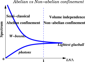
Figure 4: Cartoon of the spectral properties of the lightest glueball as a function of $LN\Lambda$. At small $LN\Lambda$, a semi-classical analysis is possible and reliable. In this regime, Abelian confinement is operative. As $N\rightarrow\infty$, this window shrinks to zero in $r(S_{1})$ and volume independence (and non-Abelian confinement) takes over at any finite $r(S_{1})$.

The quasiclassical analysis of the deformed chiral theories is reliable as long as there is a parametric separation of scales between photons (which are perturbatively massless) and the lightest $W$ bosons of the spontaneously broken non-Abelian theory. The non-perturbative photon mass and that of the lightest $W$ bosons are

$$m_{\sigma}\sim e^{-S_{0}}\sim\Lambda(\Lambda NL)^{2},\qquad m_{W}=\frac{2\pi}{LN}\,,$$ (97)

where we expressed the photon mass in the units of $\Lambda$. The photon mass is an increasing function of $LN$ while the lightest $W$-boson mass is a decreasing function as shown in Fig. 4. As long as the ratio of the two masses is smaller than unity, the large-distance dynamics can be accurately described by photons in the maximal Abelian subgroup. This implies

$$\frac{m_{\sigma}}{m_{W}}\sim(\Lambda NL)^{3}\ll 1\,.$$ (98)

At $LN\Lambda\sim 1$ the separation of scales is lost; we can no longer describe large-distance physics limiting ourselves to photons and light fermions. The theory passes from Abelian to non-Abelian confinement. At $LN\Lambda\gg 1$ the theory lacks a weak coupling description regardless of how small $r(S_{1})$ is, despite asymptotic freedom and despite the fact that we imprisoned the gauge theory in an arbitrarily small box. In a sense, the effective infrared cut-off in the case at hand is $LN$ rather than $L$. Of course, this statement is the essence of the concept of volume independence.

Thus, we see that everything fits together very well. As we make $N$ larger, the domain of validity of our analysis shrinks as $L\ll{1}/(\Lambda N)$. This is how the volume independence and quasiclassical analysis are intertwined, so that both hold without invalidating each other. Note that, were it not for the nontrivial $N$ dependence in Eq. (98), our analysis would come in contradiction with the large-$N$ volume independence. Hence, the scale $r\sim{1}/(N\Lambda)$ is an important physical scale in gauge theories – this is the scale where Abelian confinement gives place to non-Abelian confinement.

The above discussion implies that a refined (Abelian) large-$N$ limit might exist in which the combination

$$LN\Lambda=\epsilon\ll 1$$ (99)

is kept fixed and small (we must keep $\Lambda$ fixed too, of course). If the large-$N$ limit is taken according to this double scaling, physics can be described by a (compact) Abelian $[{\rm U}(1)^{\infty}]^{K}$ refined gauge structure at large distances.

In the $N=\infty$ limit, the implication of the volume independence is much stronger. It implies that all non-perturbative features, such as the glueball spectrum, string tensions, chiral condensates, etc., are independent of $r(S_{1})$. At finite $N$, physics at $L\leq{1}/(N\Lambda)$ has an $L$ dependence. The fact that the chiral condensate came out to be independent of $L$ even at small $N$ was due to the relation between $e^{-S_{0}}$ and the strong scale at the one-loop level. This might seem as a welcome one-loop beta-function accident. It is not, given that the $Z_{K}$ orbifold theories are perturbatively planar equivalent to SYM theory [7, 10], and the perturbative equivalence implies coinciding renormalization group $\beta$ function and the same strong scale by dimensional transmutation. We believe that the chiral condensates in the $Z_{K}$ orbifold theories are saturated by appropriate flux-ring operators at small $r(S_{1})$, just like the gluino condensate is saturated by the monopole operators in ${\mathcal{N}}=1$ SYM theory [29], and QCD(BF/AS/S)* [11].

6 Conclusions

The double-trace deformation gives us a controllable dynamical framework to study non-perturbative aspects of the strongly coupled chiral gauge theories. Our analysis is valid at small $r(S_{1})$. Due to the absence of a confinement-deconfinement phase transition in the deformed theories our analysis must be qualitatively valid in the chiral theories on $R_{4}$. We established, at small $r(S_{1})$, the existence of the dual photon masses generated by bions, and, hence, linear confinement. We calculated chiral condensates which determine the pattern of discrete $\chi$SB and the number of distinct vacua. The form of these condensates is in agreement with what one would naively guess assuming “minimality” and gauge invariance. At small $r(S_{1})$ they are generated by ring operators.

At small $r(S_{1})$, reduction of the full gauge symmetry down to the maximal Abelian subgroup (e.g. $[{\rm U}(1)^{N-1}]^{K}$ in the quivers) occurs in the deformed chiral theories. One of surprising findings of our work is the vanishing of the monopole operators. In other words, despite the gauge symmetry breaking, the monopoles per se do not contribute to non-perturbative dynamics. The leading non-perturbative effects are due to various flux operators, such as magnetic bions and magnetic ring operators which may be thought of as molecules built of the monopole-instantons. This is in a striking difference with YM* and QCD* theories with vector-like matter where the monopole effects are crucial.

Our work also shows that non-perturbative effects do not lead to inconsistencies in dynamics of the chiral gauge theories. In this sense, our suggestion provides an additional argument in favor of non-perturbative consistency of the chiral gauge theories.

We outlined a reduced matrix model for the large-$N$ chiral gauge theories, along the lines of working EK reductions. The main lesson here is that non-perturbative aspects (such as the spectrum) of the $N=\infty$ chiral theory on $R_{4}$ are identical to those of the reduced deformed theory on $R_{4-d}\times T_{d}$ where $T_{d}$ is a $d$-dimensional torus. A special case is a very small $T_{3}$ implying that non-perturbative spectrum of the chiral theory can be deduced by studying $N=\infty$ matrix quantum mechanics. It would be instructive to study such quantum-mechanical systems.

We also remarked that the large-$N$ volume independence and the existence of the volume dependent quasi-classical regime on $S_{1}\times R_{3}$ with small $r(S_{1})$ are not in contradiction with each other, due to non-trivial region of validity of the latter, i.e., $r(S_{1})N\Lambda\ll 1$. In the small-$r(S_{1})$ regime, Abelian confinement is operative. The volume independence is a non-perturbative property of the non-Abelian confinement regime. In our opinion, currently, the most important question in vector-like QCD* theories and deformed chiral gauge theories is to understand the transition from the Abelian to non-Abelian confinement regimes in the vicinity of $r(S_{1})\sim 1/(N\Lambda)$. The importance of this regime is due to volume independence. The physical observables of gauge theories on $R_{4}$ do get saturated by non-perturbative dynamics above the $r(S_{1})\sim 1/(N\Lambda)$ scale. After non-perturbative saturation takes place, the observables between the finite and infinite $r(S_{1})$ theories can only differ by small $O(1/N^{2})$ effects.

References

- [1]
- [2] H. Neuberger, Ann. Rev. Nucl. Part. Sci. 51, 23 (2001) [arXiv:hep-lat/0101006].
- [3] M. Lüscher, arXiv:hep-th/0102028.
- [4] M. Golterman, Nucl. Phys. Proc. Suppl. 94, 189 (2001) [arXiv:hep-lat/0011027].
- [5] E. Poppitz and Y. Shang, JHEP 0708, 081 (2007) [arXiv:0706.1043 [hep-th]].
- [6] G. ‘t Hooft, Naturalness, Chiral Symmetry, and Spontaneous Chiral Symmetry Breaking, in Recent Developments in Gauge Theories, Eds. G. ‘t Hooft et al. (Plenum Press, New York, 1980), p. 135 [Reprinted in Unity of Forces in the Universe, Ed. A. Zee (World Scientific, Singapore, 1982), Vol. II, p. 1004].
- [7] S. Kachru and E. Silverstein, Phys. Rev. Lett. 80, 4855 (1998) [arXiv:hep-th/9802183]; M. Bershadsky, Z. Kakushadze and C. Vafa, Nucl. Phys. B 523, 59 (1998) [arXiv:hep-th/9803076]; M. Bershadsky and A. Johansen, Nucl. Phys. B 536, 141 (1998) [arXiv:hep-th/9803249].
- [8] P. Kovtun, M. Ünsal and L. G. Yaffe, Phys. Rev. D 72, 105006 (2005) [arXiv:hep-th/0505075].
- [9] M. Schmaltz, Phys. Rev. D 59, 105018 (1999) [arXiv:hep-th/9805218].
- [10] M. J. Strassler, On methods for extracting exact non-perturbative results in nonsupersymmetric gauge theories, arXiv:hep-th/0104032.
- [11] M. Shifman and M. Ünsal, QCD-like Theories on : a Smooth Journey from Small to Large with Double-Trace Deformations, arXiv:0802.1232 [hep-th].
- [12] S. Dimopoulos, S. Raby and L. Susskind, Nucl. Phys. B 173, 208 (1980);
- [13] M. E. Peskin, Chiral Symmetry and Chiral Symmetry Breaking, Lectures presented at the Summer School on Recent Developments in Quantum Field Theory and Statistical Mechanics, Les Houches, France, August 1982.
- [14] A. Armoni, M. Shifman and M. Ünsal, Phys. Rev. D 77, 045012 (2008) [arXiv:0712.0672 [hep-th]].
- [15] M. Ünsal and L. G. Yaffe, Center-stabilized Yang–Mills theory: confinement and large- volume independence, arXiv:0803.0344 [hep-th].
- [16] M. C. Ogilvie, P. N. Meisinger and J. C. Myers, PoS LAT2007, 213 (2007) [arXiv:0710.0649 [hep-lat]].
- [17] J. C. Myers and M. C. Ogilvie, Phys. Rev. D 77, 125030 (2008) [arXiv:0707.1869 [hep-lat]].
- [18] P. Kovtun, M. Ünsal and L. G. Yaffe, JHEP 0706, 019 (2007) [arXiv:hep-th/0702021].
- [19] A. M. Polyakov, Nucl. Phys. B 120, 429 (1977).
- [20] T. Eguchi and H. Kawai, Phys. Rev. Lett. 48, 1063 (1982).
- [21] L. G. Yaffe, Rev. Mod. Phys. 54, 407 (1982).
- [22] G. Bhanot, U. M. Heller and H. Neuberger, Phys. Lett. B 113, 47 (1982).
- [23] G. ’t Hooft, Phys. Rev. D 14, 3432 (1976), Erratum-ibid. D 18, 2199 (1978), [reprinted in M. Shifman (Ed.), Instantons in Gauge Theories (World Scientific, Singapore, 1994), p. 70].
- [24] M. N. Chernodub and V. I. Zakharov, Phys. Rev. Lett. 98, 082002 (2007) [arXiv:hep-ph/0611228].
- [25] J. Liao and E. Shuryak, Phys. Rev. C 75, 054907 (2007) [arXiv:hep-ph/0611131].
- [26] E. Shuryak, arXiv:0807.3033 [hep-ph].
- [27] C. Callias, Commun. Math. Phys. 62, 213 (1978).
- [28] A. A. Belavin, A. M. Polyakov, A. S. Schwartz and Yu. S. Tyupkin, Phys. Lett. B 59, 85 (1975), [reprinted in M. Shifman (Ed.), Instantons in Gauge Theories (World Scientific, Singapore, 1994), p. 22].
- [29] N. M. Davies, T. J. Hollowood, V. V. Khoze and M. P. Mattis, Nucl. Phys. B 559, 123 (1999) [arXiv:hep-th/9905015].
- [30] A. Armoni, M. Shifman and G. Veneziano, Nucl. Phys. B 667, 170 (2003) [arXiv:hep-th/0302163].
- [31] A. Armoni, M. Shifman and G. Veneziano, Phys. Lett. B 579, 384 (2004) [arXiv:hep-th/0309013].
- [32] A. Armoni, M. Shifman and G. Veneziano, Phys. Rev. D 71, 045015 (2005) [arXiv:hep-th/0412203]; for reviews see A. Armoni, M. Shifman and G. Veneziano, From Super-Yang–Mills Theory to QCD: Planar Equivalence and its Implications, in From Fields to Strings: Circumnavigating Theoretical Physics, Ed. M. Shifman, A. Vainshtein, and J. Wheater (World Scientific, Singapore, 2005), Vol. 1, p. 353 [hep-th/0403071]; A. Armoni and M. Shifman, Planar equivalence 2006, in M. Gasperini and J. Maharana (Eds.), String Theory and Fundamental Interactions, (Berlin, Springer-Verlag, 2007), p. 287. [hep-th/0702045].
- [33] M. Ünsal and L. G. Yaffe, Phys. Rev. D 74, 105019 (2006) [arXiv:hep-th/0608180].
- [34] R. C. Brower, K. N. Orginos and C. I. Tan, Phys. Rev. D 55, 6313 (1997) [arXiv:hep-th/9610101].
- [35] M. Golterman and Y. Shamir, Phys. Rev. D 70, 094506 (2004) [arXiv:hep-lat/0404011].
- [36] A. Gonzalez-Arroyo and M. Okawa, Phys. Lett. B 120, 174 (1983).
- [37] B. Bringoltz and S. R. Sharpe, arXiv:0805.2146 [hep-lat].
- [38] T. Azeyanagi, M. Hanada, T. Hirata and T. Ishikawa, JHEP 0801, 025 (2008) [arXiv:0711.1925 [hep-lat]].
- [39] M. Teper and H. Vairinhos, Phys. Lett. B 652, 359 (2007) [arXiv:hep-th/0612097].
- [40]