Non-Hermitian delocalization and the extinction transition.

Abstract

Logistic growth on a static heterogenous substrate is studied both above and below the drift-induced delocalization transition. Using stochastic, agent-based simulations the delocalization of the highest eigenfunction is connected with the large $N$ limit of the stochastic theory, as the localization length of the deterministic theory controls the divergence of the spatial correlation length at the transition. Any finite colony made of discrete agents is washed away from a heterogeneity with compact support in the presence of strong wind, thus the transition belongs to the directed percolation universality class. Some of the difficulties in the analysis of the extinction transition in the presence of a localized active state are discussed.

The effect of drift on inhomogeneous systems that exhibit growth and propagation has attracted much interest in the last decade efetov ; hatano ; pik ; been ; lev ; nel ; karin ; karin1 ; ind ; pie ; lin . When the time evolution of a system is governed by a real symmetric evolution operator it may support both extended and localized eigenstates. The eigenstates of a quantum particle in a single potential well, for example, are either localized inside the wall or extended above some threshold energy. In the presence of drift, or other non-Hermitian perturbation efetov , the system undergoes a phase transition where localized wavefunctions become extended, and the corresponding eigenvalues migrate from the real axis to the complex plane. This transition was first analyzed by Hatano and Nelson hatano in the context of flux lines in high $T_{c}$ superconductors with columnar defects subjected to a tilted external magnetic field. Since then, many authors have considered this transition in different fields, e.g. hydrodynamics pik , random lasers been , and quantum dots lev among many others.

Of particular interest, both theoretically nel ; karin ; karin1 ; ind and experimentally pie ; lin , is the delocalization transition for bacterial colonies on a heterogeneous substrate in the presence of drift. A logistic growth of a motile population on a 1d static spatially heterogenous substrate is described by:

$$\frac{\partial c(x,t)}{\partial t}=D\nabla^{2}c(x,t)+v\frac{\partial c(x,t)}{\partial x}+a(x)c(x,t)-c^{2}(x,t).$$ (1)

In the absence of drift term ($v=0$) and for a homogenous environment ($a=a_{0}\equiv\sigma-\mu$, where $a_{0}$, the difference between the birth rate $\sigma$ and the death rate $\mu$, is independent of spatial location us ) one gets the celebrated Fisher-Kolomogorov-Petrovsky-Piscounov equation (FKPP), a generic description of an invasion of a stable state $(c^{*}=a_{0})$ into an unstable one $c^{*}=0$. In the asymptotic long-time limit this system supports a front that travels with constant speed $v_{F}=2\sqrt{Da_{0}}$. In the homogenous case the eigenstates of the linearized evolution operator

$${\cal{L}}=D\nabla^{2}c(x,t)+v\frac{\partial c(x,t)}{\partial x}+a_{0}c(x,t).$$ (2)

are extended sinusoidal functions and the drift corresponds to a simple Galilean transformation.

Things change when translational invariance is broken, i.e., in the presence of spatial inhomogeneity. Two main types of heterogenous growth are considered in the literature nel ; karin ; karin1 ; pie ; lin : A ”single oasis” case, where the growth rate is larger on a spatial domain, and the disordered case, where $a(x)=a_{0}+\delta a(x)$, $\delta a$ being taken from some random distribution with zero mean. In both cases the spectrum of the linear evolution operator admits localized wavefunctions; if $\{\phi^{0}_{n}(x),\Gamma_{n}\}$ is the set of eigenfunctions and the corresponding eigenvalues of ${\cal L}(v=0)$, at least some eigenstates in the tail of the spectrum (or all the states for a disordered potential below 2d) are exponentially localized. The effect of small drift on a localized eigenstates is trivial:

$$\phi^{v}_{n}(x)=e^{vx/2D}\phi^{0}_{n}(x)\quad,\quad\Gamma^{v}_{n}=\Gamma^{0}_{n}-\frac{v^{2}}{4D}.$$ (3)

This ”gauge invariance” breaks down at $v^{c}_{n}=2D/\xi_{n}$, where $\xi_{n}$ is the localization length of the $n$th eigenstate. Above $v^{c}_{n}$ the eigenstate delocalizes and the boundary conditions begin to play an important role: e.g., for periodic boundary conditions the eigenvalues that correspond to delocalized eigenstates become complex prl . The spectrum then takes the form of a ”bubble” in the complex plane, where the localized eigenstates correspond to the spectral points in the tail, since the localization length in the center of the band is larger. A non-Hermitian ”mobility edge” appears between the two regimes. Increasing $v$ even more, the bubble spreads and captures more and more spectral points, and at the end the ground state also delocalizes. The Perron-Frobenius Theorem pp ensures that the highest eigenstate stays on the real line, and the delocalization transition is identified by the breakdown of the trivial gauge (Eq. 3) and the vanishing of the spectral gap nel ; prl .

Figure 1 shows some examples of the spectrum of ${\cal L}$, together with a sketch of the phase diagram, for the single oasis scenario. In the absence of drift there is a single localized state at the right edge of the spectrum (if the oasis is large, a few localized states exist), followed by a continuum of states that correspond to extended eigenfunctions. Even a small drift is enough to push the delocalized eigenvalues to the complex plane, but the localized state only develops a slight asymmetry with almost no effect on the eigenvalue. Only for high enough drift does the highest eigenstate delocalize and the gap disappear. A change of $a_{0}$ corresponds to a rigid shift of the whole spectrum along the real line. Thus, three regimes exist in the drift-proliferation parameter space: the extinction region, where the real part of all the eigenvalues is negative; the localized region, where only the localized states admit positive growth rate; and the proliferation regime, where both localized and extended states may grow. Above $v^{c}_{0}$ only the extinction and the proliferation regions exist.

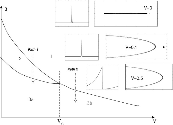
Figure 1: A sketch of the ”phase diagram” for a single oasis in the death-rate - drift space. Region (1) is the extinction region where the highest eigenvalue is negative. In region (2) only the localized state admits an eigenvalues with positive real part, and in regions (3a) and (3b) extended eigenstates become ”active”. In the right side of the figure the highest eigenstate and the spectrum in the complex plane are plotted for the cases of no drift ($v=0$), small drift ($v=0.1$) and large drift ($v=0.5$) for a single oasis.

The above discussion is, however, too naive. Bacterial systems are not deterministic, and are composed of discrete objects that may die, reproduce or migrate with some probability that depends on the local environmental conditions. The bacterial population at a certain point is not a deterministically varying continuous quantity, like $c(x)$, but a discrete number that undergoes stochastic processes, e.g., $A\to 2A,\ A+A\to\emptyset,\ A\to\emptyset$ etc. Like in many other branches of science, the deterministic dynamics is an approximate description of the system that becomes exact where the effect of stochasticity vanishes. In the case considered here the demographic stochasticity becomes negligible when the density of agents is large, since the relative fluctuations scale with $1/\sqrt{N}$. Technically, the exact stochastic Master equation is replaced by a deterministic description using the Kramers-Moyal expansion, or more rigorously by van-Kempen’s $\Omega$ expansion and related methods vk ; gardiner . Joo and Lebowitz joo have already pointed out that in the limit of large $N$ one should expect a population density distribution that follows the spatial features of the active eigenstates, i.e., the eigenstates for which $Re(\Gamma)>0$. Here, on the other hand, we want to discuss the effects of spatial heterogeneity and drift for a dilute system; i.e., close to the extinction transition. In that case the $1/\sqrt{N}$ expansions are invalid and so we resort to numerical simulations.

Let us first present some general considerations. Grassberger and Janssen jan suggested long ago that the extinction transition to a single absorbing state on a homogenous substrate belongs (in the absence of special additional symmetries) to the directed percolation (DP) equivalence class, independent of the microscopic details of the stochastic process. DP is a continuous transition and the correlation length and correlation times diverge at the transition point with their characteristic exponents (see 1 for a general review). On a homogenous substrate the correlation length is the only length scale of the problem. On a static heterogenous substrate, on the other hand, another length scale appears - the localization length. How do these two quantities relate to each other? What are the properties of the stochastic extinction transition below and above the deterministic delocalization transition? In what sense is Eq. (1) a deterministic limit of a stochastic process when the effect of stochasticity is important; i.e., close to the extinction transition?

Recently, this last question has been addressed for the transition on a homogenous substrate kessler . It turns out that the transition is always in the DP equivalence class, but the carrying capacity of the system, N, determines the location of the transition and, more important, the width of the transition zone. In the deterministic theory the correlation length is zero both below and above the transition (any initial density fluctuation simply decays exponentially to the stable state and its spread during this process is negligible). The spatial correlation length for the stochastic process satisfies $\xi_{\perp}\sim\Delta^{-\nu_{\perp}}/N^{\kappa}$, where $\Delta$ is the distance from the transition. If the system parameters are such that its deterministic analogue is at the transition point, then $\Delta(N)\sim N^{-\tau}$ and $\Delta$ vanishes at the deterministic limit. Under these conditions $\xi_{\perp}\sim N^{\gamma}$, where $\gamma=\tau\nu_{\perp}-\kappa$. This implies that for any finite $\Delta$ for large enough $N$ the correlation length shrinks to zero and the deterministic description holds, whereas for any finite $N$, for small enough $\Delta$ the system enters the transition zone and the deterministic description collapses. Both $\kappa$ and $\tau$ depend on the deterministic features of the model as explained in kessler , but in any case $\gamma>0$ so the deterministic limit never exists at the transition point.

In order to simulate the heterogenous system in the large $N$ limit, an individual based model that allows for an accurate determination of the transition point in the $N\to\infty$ limit is used. We consider a logistic growth process on a one dimensional lattice with periodic boundary conditions; Euler integration is used with small, but finite, $\Delta t$. The number if agents at the $i$-th lattice site is an integer $n_{i}$, and each cycle of the Monte-Carlo simulation involves two consecutive steps. The first step is the reaction: each of the agents at the site produces an offspring with probability $(\sigma_{0}+\delta\sigma_{i})(1-n_{i}/N_{0})\Delta t$, and dies with probability $\mu\ \Delta t$. In the second, diffusion step, any agent is selected for migration with probability $2\chi\Delta t$, then chooses its destination - to the left with probability $q_{L}=(1+\nu)/2$ or to the right with probability $1-q_{L}$. To avoid artificial drift as a result of the sequential update of lattice sites, parallel update was used; $n_{i}$ is updated only after the diffusion cycle is completed.

In the linearized deterministic limit this model corresponds to an $L$ dimensional map, where $L$ is the number of sites. This map is given by the multiplication of the reaction matrix, $R_{i,j}=\delta_{i,j}[1+\Delta t(\sigma_{0}+\delta\sigma_{i}-\mu)]$, by the diffusion matrix that takes the form (up to the boundary conditions) $D_{i,j}=\delta_{i,j}(1-2\chi\Delta t)+\delta_{i,j+1}\chi(1+\nu)\Delta t+\delta_{i+1,j}\chi(1-\nu)\Delta t$. Diagonalizing the product $DR$ one finds the highest eigenvalue $\tilde{\Gamma}_{0}$ and the corresponding eigenvector, $\phi_{0}^{i}$; adding another death process, where each particle in the MC simulation is selected to die after any cycle with probability $1/\\ tilde{Gamma}_{0}$, ensures that the system is exactly at the transition point for $N_{0}\to\infty$. In different words, the agent-based system is simulated with a parameter set that ensures $\Gamma_{0}=0$ in the deterministic limit.

Clearly, a system with finite carrying capacity $N_{0}$ is always closer to extinction than the deterministic system when all other parameters are equal. This implies that, scaling the parameters as described above and increasing $N_{0}$, the system is always in the extinction phase and reaches the transition exactly at $N_{0}=\infty$. In Fig. 3, $\xi_{\perp}$, the correlation length, is plotted vs. $N_{0}$ on a log-log scale and reveals the real meaning of the deterministic delocalization transition: below $v_{c}$, i.e., when $\phi_{0}$ is localized, the correlation length associated with the stochastic process first grows and then saturates to the deterministic localization length $\xi/[1-v\xi/(2D)]$. This demonstrates the fact that the state that becomes active at the transition is localized and the correlation length of the stochastic process can not grow beyond this deterministic length.

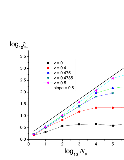
Figure 2: The log of the transverse correlation length $\xi_{\perp}$ (in the direction of the drift) vs. $log(N_{0})$ for a system of length $L=2000$. Here $\xi=0.2,\sigma_{0}=\mu=1$ and the heterogeneity $\delta\sigma_{i}=0.2\delta_{i,L/2}$.

On the other hand, above $v_{c}$ the correlation length grows unboundedly with $N_{0}$. The data is consistent with $\xi_{\perp}\sim N_{0}^{0.5}$, which is (up to logarithmic corrections), the lifetime of a well-mixed system at the deterministic transition point san . This reflects the fact that the delocalized system is not really one dimensional but rather $"0+1"$ dimensional, with the spatial direction playing the role of time. Life in that system is a result of a drift from a source, not of uniform growth, and the lifetime of the colony at the oasis determines the spatial extent reached by its decedents.

For finite $N_{0}$ and with constant drift velocity $v$, the system undergoes undergone an extinction transition as $a_{0}$ decreases. This may happen either via the localized phase (e.g., along Path 1 shown by the arrow in Figure 1), or directly to the delocalized phase (Path 2 in figure 1). While for $N_{0}\to\infty$ the transition happens when $Re(\Gamma_{0})$ touches zero, for any finite $N_{0}$ the transition takes place when a finite region of the upper part of the spectrum is above zero (inset of Fig. 3). For a single oasis (or otherwise when the number of oases is finite) all the localized states decay in the long run as a result of demographic stochasticity; only when the extended eigenstates are ”excited” (their eigenvalues cross to the positive real part of the spectrum) will the system be in its active phase. As a result, the scenarios 1 and 2 can be seen to differ significantly.

Let us first consider path 2. Intuitively, above $v_{c}$ the colony is carried off the oasis by the wind, thus the large-scale properties of the system are identical with a homogenous substrate with drift in the thermodynamic limit. More precisely, for finite $N_{0}$ the transition occurs when a finite part of the spectrum, made of delocalized states, is already ”excited” (i.e., $Re(\Gamma)>0$ for the these eigenstates). Thus, there are two regimes. Deep in the extinction phase all states decay, $Re(\Gamma)<0$. The bacterial density in this regime satisfies the deterministic solution $c(x,t)=\exp(-|a_{0}|t-(x-x_{0}-vt)^{2}/4Dt)/\sqrt{4\pi Dt}$, where $x_{0}$ is the nucleation point. The overall occupation of a point, $C_{T}(x)\equiv\int c(x,t)\ dt$, is thus a monotonically decreasing function of $x-x_{0}$, with an exponential decay of the tail $C_{T}(x)\sim exp(-(x-x_{0})/\xi)$, where the localization length $\xi$ scales like $D/(\sqrt{v^{2}+2D|a_{0}|}-v)$.

Close to the transition point for finite $N_{0}$, on the other hand, many linear states are already excited and the growth of the colony is unaffected by the nonlinear competition at short times. Only after the characteristic time $\xi_{\|}$ does nonlinearity suppress the growth, leading to extinction. Within this growth period the system behaves deterministically and a ”Fisher front” starts to invade the empty region. As the wind velocity is larger than the Fisher velocity above $v_{c}$ nel , the maximum of $C_{T}(x)$ moves in the direction of the wind, as demonstrated in Figure 3. This second regime vanishes at the deterministic limit; accordingly, the detachment of the peak from the nucleation point disappears upon increasing $N_{0}$.

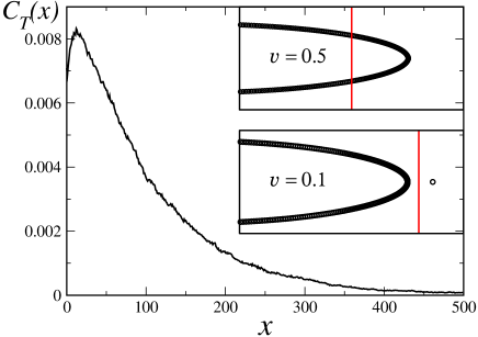
Figure 3: $C_{T}(x)$ vs. $x$ close to the transition ($\beta=0.19$, $v=0.7$, other parameters identical with those used in Fig. 2) for $N_{0}=3$. The effect of the localized heterogeneity at $x=0$ is almost unseen. As emphasized in the upper inset, the transition takes place when many delocalized modes are also excited; as a result the system initially grows and the colony pushed to the right by the wind, yielding a hump away from the oasis. This peak disappears for larger $\beta$ and for larger $N_{0}$ (results not shown). The lower inset exemplify the spectrum of the linearized evolution operator when the transition takes place along path 1 of Figure 1.

The situation is completely different along path 1. The highest state is now localized, and its nonlinear interaction differs substantially from the interaction between extended states. If the localization length is finite the oasis region decouples from the rest of the system in the thermodynamic limit and the DP dynamics happens in parallel with the zero dimensional stochastic process on the oasis. This decoupling, however, is impossible at the bulk DP transition, when $\xi_{\bot}$ diverges hi . A related issue is the transition in the presence of a finite density of randomly distributed oases: below $v_{c}$ a nonuniversal Griffiths phase appears between the active and the inactive parameter regions ga . In the deterministic limit only the highest localized state becomes active at the transition, thus the Griffith phase admits no deterministic limit, and its width shrinks to zero. These last two observations suggest that the deterministic description of the system by means of excited localized eigenstates is insufficient, as the convergence of a finite $N$ system to the deterministic limit is a very subtle issue, to be addressed in subsequent publication.

- (1) K. B. Efetov, Phys. Rev. Lett. 79, 491 (1997); Phys. Rev. B 56, 9630 (1997).
- (2) N. Hatano and D. R. Nelson, Phys. Rev. Lett. 77, 570 (1996); Phys. Rev. B 56, 8651 (1997).
- (3) A. V. Straube and A. Pikovsky, Phys. Rev. Lett. 99, 184503 (2007).
- (4) C. W. J. Beenakker, J. C. J. Paasschens, and P. W. Brouwer, Phys. Rev. Lett. 76, 1368 (1996).
- (5) M. S. Rudner and L. S. Levitov, cond-mat/0807.2048
- (6) D. R. Nelson and N. M. Shnerb, Phys. Rev. E 58, 1383 (1998).
- (7) K. A. Dahmen, D. R. Nelson, and N. M. Shnerb, J. Math. Biol. 41, 1 (2000); K. A. Dahmen, D. R. Nelson, and N. M. Shnerb, in Statistical Mechanics of Biocomplexity, edited by D. Reguera, J. M. G. Vilar, and J. M. Rubi (Springer, Berlin, 1999).
- (8) A.R. Missel and K.A. Dahmen, Phys. Rev. Lett. 100, 058301 (2008).
- (9) V. M. Kenkre and N. Kumar, cond-mat/0808.0172.
- (10) T. Neicu, A. Pradhan, D. A. Larochelle, and A. Kudrolli, Phys. Rev. E 62, 1059 (2000); N.M. Shnerb, Phys. Rev. E 63, 011906 (2000).
- (11) A.L. Lin, B.A. Mann, G. Torres-Oviedo, B. Lincoln, J. Käs and H. L. Swinney, Biophysical Journal 87, 75-80 (2004).
- (12) Althogh in the deterministic limit, simply shifts , it is important to include an explicit death term in the microscopic theory, as explained in kessler .
- (13) N. M. Shnerb and D. R. Nelson, Phys. Rev. Lett. 80, 5172 (1998).
- (14) H. K. Janssen, Z. Phys. B 42, 151 (1981); P. Grassberger, Z. Phys. B 47, 365 (1982).
- (15) Bapat, R.B. and Raghavan, T.E.S., Nonnegative Matrices and Applications, Encyclopedia of Mathematics and its Applications, (Cambridge University Press, Cambridge, 1997).
- (16) J. Joo and J.L. Lebowitz, Phys. Rev. E 72, 036112 (2005).
- (17) N. G. van Kampen, Stochastic Processes in Physics and Chemistry, Third Edition, (Elsevier, Amsterdam, 2007).
- (18) C. W. Gardiner, Handbook of Stochastic Methods for Physics, Chemisty and the Natural Sciences, Third Edition, (Springer-Verlag, Berlin, Heidelberg, New York, 2004).
- (19) H . Hinrichsen, Adv.Phys. 49, 815-958 (2000).
- (20) C. R. Doering, K. V. Sargsyan, and L. M. Sander, Multi-scale Model. Simul. 3, 283 (2005).
- (21) D. Kessler and N.M. Shnerb, J. Phys. A 41, 292003 (2008).
- (22) See, in this regard, A.C. Barato and H. Hinrichsen, cond-mat/0802.3580.
- (23) A.G. Moreira and R. Dickman, Phys. Rev. E 54 R3090 (1996).