Stochastic Resonance in an Overdamped Monostable System.

Abstract

We show, the SR can appear in monostable overdamped systems driven by additive mix of periodical signal and white Gaussian noise. It can be observed as non-monotonic dependence of SNR on the input noise intensity. In this sense it is similar to classical SR observed in overdamped bistable systems with potential barrier.

The dynamics of nonlinear periodically driven stochastic systems has been attracted great attention during the last decades . The interest in these systems is much stimulated by phenomenon known as stochastic resonance (SR), where noise plays a constructive role Anishchenko02 ; Gammaitoni98 . This phenomenon can be defined as enhancement of sensitivity of a nonlinear system to external periodical forcing. Nowadays the SR has been found and studied in a different physical, chemical and biological systems Dykman95 ; Greenwood00 ; Guo06 ; Mitaim98 ; Vilar99 ; Jung02 ; Zozor03 ; Valenti04 ; Spagnolo02 . The enhancement of sensitivity is usually understood as nonmonotonic dependence of the signal-to-noise ratio (SNR) or signal power amplification (SPA) at the output of nonlinear system as a functions of the input noise intensity. Accordingly, the phenomenon of SR displays itself, when SNR and SPA reach maximum at some value of noise intensity and then decrease with further growth of fluctuations.

The effect of SR was observed in various monostable systems: with multiplicative noise Guo06 , signal array Lindner01 , underdamped Stocks93 , higher harmonics Grigorenko97 . The present paper is dedicated to the investigation of monostable systems described by the overdamped Langevin equation with an additive noise and an additive driving signal

$${{dx}\over{dt}}=-{{d\Phi(x)}\over{dx}}+s(t)+\xi(t),$$ (1)

where $s(t)=A\cos(\omega_{0}t)$ is the input driving signal, $\xi(t)$ is the input white Gaussian noise: $<\xi(t)>=0$, $<\xi(t)\xi(t+\tau)>=2q\delta(\tau)$, $2q$ is the noise intensity, $\Phi(x)$ is potential field describing the system and $x(t)$ is the output random process.

The canonical example of SR was observed and studied in overdamped system (1) for the bistable potential profile $\Phi(x)$ with single potential barrier separating the metastable states in Refs.Anishchenko02 ; Gammaitoni98 ; McNamara89 . This result can be generalized for multistable potentials with arbitrary number of barriers. The value of additive noise intensity for which SNR reaches the maximum was revealed to be about the height of the potential barrier. In other words, the presence of potential barrier(s) has been considered as necessary condition for arising of SR in overdamped systems with additive noise (1). It is well known also that in bistable (multistable) systems the non-monotonic dependence of SNR is accompanied by the similar non-monotonic dependence of SPA on noise intensity.

Recently, in Ref. Evstigneev04 it was shown that some special kind of SR can appear in overdamped monostable systems (1), where there is no any barriers in potential profile $\Phi(x)$. This kind of SR is different from classical one, because the non-monotonic dependence on the noise intensity is observed only for SPA. While the SNR was shown to be monotonically decreasing function of the noise intensity regardless to various non-monotonic dependencies of SPA Agudov08 .

In the present Letter we demonstrate that the non-monotonic dependence of SNR, similar to that for bistable systems, can be observed also in monostable overdamped systems. This result implies the presence of SR in monostable overdamped system with additive noise and signal. For this case the maximum of SNR for non-zero noise level has never been observed before. On the other hand, this situation is sufficiently general to be achieved in a great vaiety of physical, chemical, and biological systems.

The function of SNR is obtained analytically. The analysis of the SNR and SPA shows that this phenomenon of SR is new and it has different properties comparing to the classical case appearing in the systems with barriers.

Consider the following piece-wise linear monostable potential (See Fig. 1)

$$\Phi(x)=\left\{\begin{array}[]{ll}k_{1}|x|,&|x|<L,\\ k_{2}(|x|-L)+k_{1}L,&|x|>L.\end{array}\right.$$ (2)

Figure 1: Piece-wise linear monostable potential $\Phi(x)$.

This potential profile is monostable and has two parameters specifying the slope of potential profile wells: $k_{1}$ describes the slope near the minimum at $|x|<L$ and $k_{2}$ for $|x|>L$. The both values $k_{1}$ and $k_{2}$ are always positive providing the monostability (single minimum) of potential $\Phi(x)$, while $k_{1}$ can be grater than $k_{2}$ and vice versa.

For derivation of the power spectrum density (PSD) of the output signal $x(t)$ the linear response theory (LRT) is used assuming that the magnitude $A$ of driving signal $s(t)$ is small enough: $A\ll\min\{k_{1},k_{2}\}$. In accordance with LRT (See for example Ref. Anishchenko02 ) the PSD of the output process $x(t)$ reads

$$S_{x}(\omega)=S_{x}^{(0)}(\omega)+{{a^{2}}\over{4}}\left(\delta(\omega-\omega_{0})+\delta(\omega+\omega_{0})\right).$$ (3)

The function $S^{(0)}_{x}(\omega)$ provides the noise platform and the other term is the output signal with amplitude $a$. Therefore the SNR is defined as follows Anishchenko02

$$R={{a^{2}}\over{2S_{x}^{(0)}(\omega_{0})}}.$$ (4)

The function $S^{(0)}_{x}(\omega)$ is the PSD of the unperturbed system (1) under $s(t)=0$, which is defined as the Fourier transform of the appropriate unperturbed autocorrelation function

$$S_{x}^{(0)}(\omega)={1\over\pi}\int\limits_{0}^{\infty}K_{x}^{(0)}[\tau]cos(\omega\tau)d\tau,$$ (5)

where $K_{x}^{(0)}[\tau]=\left<x(t)x(t+\tau)\right>$. In the above expression we have taken into account that $K_{x}^{(0)}[\tau]$ is even function. According to the LRT, the amplitude of output signal is

$$a=A|\chi(i\omega_{0})|,$$ (6)

where $\chi(i\omega)$ is the susceptibility of the system. Therefore SPA of input signal $s(t)$ reads

$$\eta={a^{2}\over A^{2}}=|\chi\left(i\omega_{0}\right)|^{2}.$$ (7)

The susceptibility is the Fourier transform of linear response function $h(\tau)$

$$\chi(i\omega)=\int\limits_{-\infty}^{\infty}h(\tau)e^{-i\omega\tau}d\tau,$$ (8)

while the linear response function can be expressed in terms of correlation function of unperturbed system in accordance with fluctuation-dissipation theorem

$${h(\tau)}=-{{\theta(\tau)}\over{q}}{{dK_{x}^{(0)}[\tau]}\over{d\tau}},$$ (9)

where $\theta(\tau)$ is the Heaviside function.

The probability density function (PDF) of the unperturbed process $W^{(0)}(x,t)$ satisfies the Fokker-Planck equation (FPE) Risken89

$${{\partial{W^{(0)}(x,t)}}\over{\partial{t}}}={\partial\over\partial x}\left({d\Phi(x)\over{dx}}W^{(0)}(x,t)+\right.$$ (10)

$$\left.+q{\partial{W^{(0)}(x,t)}\over\partial{x}}\right)$$

with boundary conditions $W^{(0)}(\pm\infty,t)=0$. Since we consider $\Phi(x)\to\infty$ under $x\to\pm\infty$, the stationary PDF will be established in the system with time

$$W_{st}^{(0)}(x)=N\exp\left(-{\Phi(x)\over q}\right),$$ (11)

where $N$ is the normalization factor. Therefore to find autocorrelation function

$$K_{x}^{(0)}[\tau]=\int\limits_{-\infty}^{\infty}x_{0}W_{st}^{(0)}(x_{0})dx_{0}\int\limits_{-\infty}^{\infty}xW^{(0)}(x_{0}|x,\tau)dx.$$ (12)

it is necessary to obtain the transition probability density $W^{(0)}(x_{0}|x,t)$, which is the solution of FPE (10) with the initial conditions $W^{(0)}(x,0)=\delta(x-x_{0})$.

For the real physical system the integration in Eq. (8) can be not from $-\infty$ but from $0$, because linear response function, according to Eq. (9), exists only if $\tau>0$. Therefore susceptibility $\chi(i\omega)$ in Eq. (8) can be considered as the Laplace transform of the linear response function

$$\chi(p)=\hat{h}(p)=\int_{0}^{\infty}h(\tau)e^{-p\tau}d\tau,$$

where $p=i\omega$ is the Laplace variable. On the other hand, we can find Laplace transform of the linear response function by integrating the expression (9) and finally we obtain

$$\chi(i\omega)={1\over{q}}\left(K_{x}^{(0)}[0]-i\omega\hat{K}_{x}^{(0)}[i\omega]\right),$$ (13)

where $K_{x}^{(0)}[0]$ is the correlation function at $\tau=0$

$$K_{x}^{(0)}[0]=\langle x^{2}\rangle+m^{2}_{st},$$ (14)

which is expressed in terms of variance and mean value of the stationary distribution (11). The PSD (5) also can be written as the real part of the Laplace transform $\hat{K}_{x}^{(0)}[p]$

$$S_{x}^{(0)}(\omega)={1\over\pi}\mathbf{Re}\left\{\hat{K}_{x}^{(0)}[i\omega]\right\}.$$ (15)

In the present paper the Laplace transform of autocorrelation function is obtained for monostable potential (2). The Laplace transform method for solution of the FPE is described in Refs. Atkinson68 ; Agudov93 ; Malakhov96 ; Privman91 . In particular, in Ref. Agudov93 the exact Laplace transform of transition probability density is obtained for piece-wise linear potential profile consisting of an arbitrary number of linear parts. Using this approach we obtain the following exact expression for Laplace transform of unperturbed autocorrelation function

$$\hat{K}_{x}^{(0)}[p]={{\langle x^{2}\rangle}\over{p}}+{{\sum\limits_{i=0}^{9}A_{i}}\over{B}},$$ (16)

where coefficients $A_{i}$ are as follows

$${\langle x^{2}\rangle}={{q}\over{2p\beta\delta^{2}}}{{2+2h\delta+h^{2}\delta^{2}-\left(h^{2}+2h+2\lambda\right)\delta^{3}}\over{1-\lambda\delta}},$$

$$A_{0}={{4q\beta\lambda\mu\left(1-4\delta\right)}\over{\left(1-\lambda\delta\right)}},$$

$$A_{1}=-{{8q\beta\left(1-\delta\right)\left(\left(1-\lambda\right)\alpha_{1}^{2}+\alpha_{2}^{2}\right)\gamma_{1}}\over{\left(1-\lambda\delta\right)}},$$

$$A_{2}={{2q\left(2\lambda\mu\left(2-\delta\right)-4\delta\mu+\delta\lambda\left(2-\mu\right)\gamma_{1}\right)}\over{\left(1-\lambda\delta\right)}},$$

$$A_{3}=-{{4q\gamma_{1}\left(\left(2-\delta\right)\alpha_{2}^{2}+\delta\lambda\left(2+\left(2-\mu\right)\gamma_{2}\right)\right)}\over{\delta^{2}\left(1-\lambda\delta\right)\left(1+\gamma_{2}\right)}},$$

$$A_{4}=-{{4q\gamma_{1}\alpha_{1}^{2}\left(2-3\delta\right)\left(1-\lambda\right)}\over{\delta^{2}\left(1-\lambda\delta\right)\left(1+\gamma_{2}\right)}},$$

$$A_{5}={{2q\mu\left(\left(2-\delta\right)\lambda+2\delta\left(2-\lambda\right)\gamma_{2}+2\delta\left(1-\lambda\right)\right)}\over{\delta^{2}\left(1-\lambda\delta\right)\left(1+\gamma_{2}\right)}},$$

$$A_{6}={{q\gamma_{1}\left(2-\mu\right)\left(\delta\lambda\left(1+\gamma_{2}\right)-6+2\delta-2\gamma_{2}\right)}\over{\beta\delta^{2}\left(1-\lambda\delta\right)\left(1+\gamma_{2}\right)}},$$

$$A_{7}={{2q\mu\left(1+\delta\left(2-\lambda\right)-2\delta^{2}\lambda\right)\gamma_{2}}\over{\beta\delta^{2}\left(1-\lambda\delta\right)\left(1+\gamma_{2}\right)}},$$

$$A_{8}={{2q\mu\left(3+4\lambda-2\delta^{2}\lambda-\delta\left(2+3\lambda\right)\right)}\over{\beta\delta^{2}\left(1-\lambda\delta\right)\left(1+\gamma_{2}\right)}},$$

$$A_{9}={{4q\mu}\over{\beta^{2}\delta^{3}\left(1+\gamma_{2}\right)}},$$

$$B=p^{2}\left(1+\gamma_{2}\right)^{2}\left(\left(2-\mu\right)\gamma_{2}-\mu\left(1-\delta+\delta\gamma_{2}\right)\right),$$

here $h={{k_{1}L}/{q}}$, $\beta={{k_{2}^{2}}/{2pq}}$, $\gamma_{1}=\sqrt{1+{{4pq}/{k_{1}^{2}}}}$, $\gamma_{2}=\sqrt{1+{{4pq}/{k_{2}^{2}}}}$, $\delta={{k_{2}}/{k_{1}}}$, $\lambda=1-e^{h}$, $\mu=1-e^{h\gamma_{1}}$, $\alpha_{1}=\sqrt{1-\mu}-{{1}/{\sqrt{1-\lambda}}}$, $\alpha_{2}=\sqrt{1-\mu}-\sqrt{1-\lambda}$.

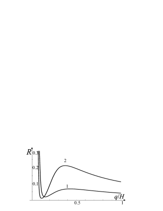
Figure 2: The SNR of the system (1) with monostable potential (2) versus dimensionless noise intensity $q/H$ for the amplitude of input signal $A=0.3$ and frequency $\omega_{0}=0.1$. The Curve 1 corresponds to $k_{1}=25$, $k_{2}=3$, $L=0.2$ and Curve 2 corresponds to $k_{1}=20$, $k_{2}=1$, and $L=0.1$.

With the above exact expression for autocorrelation function (16) we can obtain the PSD (15) and the SNR (4). In Fig. 2 the SNR is plotted versus the dimensionless input noise intensity $q/H$ for different values of $L$ and the slopes $k_{1}$, $k_{2}$. Namely, curve 1 is for $L=0.2$, $k_{1}=25$ and $k_{2}=3$, curve 2 is for $L=0.1$ and $k_{1}=20$ and $k_{2}=1$. The value $H=k_{1}L$ is the parameter of the potential profile (2) (See the Fig. 1). As one can see from Fig. 2, for small and large $q$, the SNR is decreasing function of $q$ similar to the other cases of monostable potentials considered earlier in Ref. Agudov08 . While for the intermediate values of noise intensity $0.1H\leq q\leq 0.4H$ the non-monotonic behavior of the SNR appears. It looks similar to the effect of the SR observed in bistable systems with barrier (See for example Refs. Anishchenko02 ; Gammaitoni98 ).

The properties of this SR behavior are varying, depending on the values of parameters of the investigated monostable potential profile (2). The effect is observed when $k_{1}>3k_{2}$. It follows from Fig. 2, that the maximum of SNR is reached at noise intensity $q^{*}\simeq 0.4H$. The difference between the values of SNR in the maximum and in the minimum is growing with the difference between $k_{1}$ and $k_{2}$. In particular, for the Curve 2 in the Fig. 2 we can see the improvement in SNR about 10 times with increasing of input noise from $q=0.1H$ up to $q^{*}=0.4H$.

In spite of the similar manifestation, the mechanism of this SR should be different from that in bistable systems, where the key parameter of the SR effect is the height of potential barrier. In the considered monostable system there is no barrier and the force, which is regular in time, always tends to return the system to the equilibrium point $x=0$, corresponding to the minimum of potential profile (2). The SR appears for the special shape of potential profile, which defines the strength of the regular force. Namely, the regular returning force should be much weaker in the area located far from equilibrium point comparing to that being near the equilibrium. For the potential (2) the strength of the force is changed in the points $x=\pm L$. If this change is large enough $k_{2}<3k_{1}$, the SR can be observed as a maximum of SNR as a function of the noise intensity.

Such a shape of potential profile provides the system properties, which are similar to those for excitable systems, where the SR also was observed Gammaitoni98 ; Longtin93 ; Longtin98 . The excitable systems also have only one stable state. Under a small perturbation these systems relax quickly to the stable state. While a large (over threshold) perturbation switches system to an excited state. The exited state is not stable and it decays to the stable state but after relatively longer time. For the potential profile (2) when $k_{1}\gg k_{2}$ the system (1) returns to the stable state relatively quickly, if a perturbation is less than $L$. When a perturbation exceeds the threshold value $L$, the system delays in the region $|x|>L$ for a relatively longer time, because the returning force there is weak. On the other hand, the similarities between the investigated and excitable systems are only qualitative. The equations describing excitable and threshold systems are different from Eq. (1).

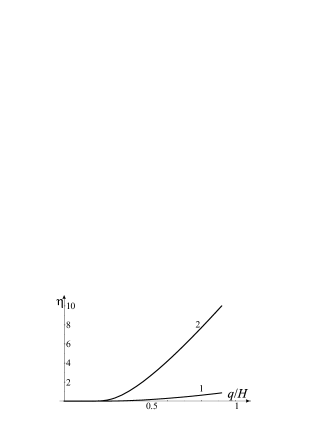
Figure 3: The SPA of the system (1) with monostable potential (2) versus dimensionless noise intensity $q/H$ for the amplitude of input signal $A=0.3$ and frequency $\omega_{0}=0.1$. The Curve 1 corresponds to $k_{1}=25$, $k_{2}=3$, $L=0.2$ and Curve 2 corresponds to $k_{1}=20$, $k_{2}=1$, and $L=0.1$.

The properties of the SR effect observed here for the monostable potential (2) has another important difference from the SR in bistable systems. In accordance with analysis carried out by various authors, in bistable (and multi-stable) systems the non-monotonic behavior of the SNR with the input noise is accompanied by similar behavior of the SPA. Using the Laplace transform of the autocorrelation function (16), we can obtain the SPA for the investigated monostable system. The plot of SPA as a function of the input noise intensity is shown in Fig. 3. The parameters of the system for the Curves 1 and 2 in the Fig. 3 are the same as those in Fig. 2, where the plots of SNR are presented. One can see, the non-monotonic dependence of SNR corresponds to the monotonically growing behavior of SPA as a function of noise intensity.

This diversity in the properties for the SR in bistable and monostable systems confirms the assumption about different mechanisms for the SR effect in these systems. Therefore we can conclude that the SR effect presented here is new and needs further detailed analysis.

The authors acknowledge fruitful discussions with Bernardo Spagnolo. This work is supported by Russian Foundation for Basic Research (project 08-02-01259).

References

- (1) V.S.Anishchenko, Nonlinear dynamics of chaotic and stochastic systems. - Berlin: Springer 2002.
- (2) L.Gammaitoni, P.Hänggi, P.Jung and F.Marchesoni, Reviews of Modern Physics 70 (1), 223 (1998).
- (3) M.I.Dykman, T.Horita, J.Ross, J.Chem.Phys. 103, 966 (1995).
- (4) P.E.Greenwood, L.M.Ward, D.F.Russell, A.Neiman and F.Moss, Phys.Rev.Lett. 84 (20), 4773 (2000).
- (5) F.Guo, Y.R.Zhou, S.Q.Jiang and T.X.Gu, J.Phys.A: Math.Gen 39, 13861 (2006).
- (6) P.Jung, Chem. Phys. Chem 3, 285 (2002).
- (7) S.Mitaim and B.Kosko, Proceedings of the IEEE 86 (11), 2152 (1998).
- (8) J.M.G.Vilar, R.V.Solé and J.M.Rubí, Phys.Rev.E 59 (5), 5920 (1999).
- (9) S.Zozor, P-O.Amblard, IEEE Transaction on signal processing 51, 3177 (2000).
- (10) D. Valenti, A. Fiasconaro, B. Spagnolo, Physica A 331, 477 (2004).
- (11) B. Spagnolo, M.Cirone, A. La Barbera, F. de Pasquale, J. Phys. Cond. Matt. 14, 2247 (2002).
- (12) J.F.Lindner, B.J.Breen, M.E.Wills, A.R.Bulsara and W.L.Ditto, Phys.Rev.E 63, 051107 (2001).
- (13) N.G.Stocks, N.D.Stein and P.V.E.McClintock, J.Phys.A:Math.Gen. 26, L385 (1993).
- (14) A.N.Grigorenko, S.I.Nikitin and G.V.Roschepkin, Phys.Rev.E 56 (5), R4907 (1997).
- (15) B. McNamara and R. Wiesenfeld, Phys. Rev. E 39, 4854 (1989)
- (16) N.V.Agudov and A.V.Krichigin, International Journal of Bifurcation and Chaos 18 (2008).
- (17) M.Evstigneev, P.Reimann, V.Pankov and R.H.Prince, Europhys.Lett. 65 (1), 7 (2004).
- (18) H.Risken, The Fokker-Planck Equation. Methods of Solution and Applications. - Berlin: Springer-Verlag 1989.
- (19) J.D.Atkinson and T.K.Caughey, Int.J.Non-Linear Mech 3, 137 (1968).
- (20) N.V. Agudov and A.N. Malakhov, Radiophysics and Quantum Electronics, 36, 97 (1993).
- (21) A.N.Malakhov and A.L.Pankratov, Physica A 299, 109 (1996).
- (22) V.Privman and H.L.Frisch, J. Chem. Phys 94, 8216 (1991).
- (23) A. Longtin, J. Stat. Phys. 70, 309 (1993).
- (24) A. Longtin and D.R. Chialvo, Phys. Rev. Lett. 81, 4012 (1998).