Why phase diagrams of different underdoped cuprates are remarkably different? Disorder versus bilayer.

Abstract

Contrary to a widely accepted view the phase diagrams of La_2-xSr_xCuO₄ and YBa₂Cu₃O_6+y, in spite of similarities are remarkably different. Both the electric conduction properties and the commensurate/incommensurate spin ordering properties differ dramatically. It is argued that the role of disorder in YBCO is insignificant while the bilayer structure is crucial. On the other hand in LSCO the intrinsic disorder to a large extent drives the properties of the system. The developed approach explains the low-temperature magnetic properties of the systems. The most important point is the difference with respect to the incommensurate spin ordering, including the difference in the incommensurate pitches. The present analysis demonstrates that the superconductivity is intimately related to the incommensurate spin ordering.

In early days of high temperature superconductivity there was a belief that the phase diagram of La_2-xSr_xCuO₄ (LSCO) represents a generic phase diagram of cuprate superconductors. Nowadays it has become clear that, in spite of similarities, there are very important differences between different cuprates. LSCO and YBa₂Cu₃O_6+y (YBSO) are the best experimentally studied compounds in the low doping regime. This is why the present work addresses these compounds. In LSCO the doping level of CuO₂-planes $p$ practically coincides with Sr concentration, $p\approx x$, while in YBCO, because of the partial filling of oxygen chains, the doping level is different from the oxygen concentration y. In LSCO doping gives way to superconductivity at $p>p_{sc}\approx 0.055$ and in YBCO at $p>p_{sc}\approx 0.065$, see Fig. 1. At first sight this indicates full similarity. However, I will argue that the mechanisms behind $p_{sc}$ in those two compounds are different and the closeness of the two values of $p_{sc}$ is purely accidental. An important observation is that the normal state electrical resistivities at $p<p_{sc}$ are very much different. At low temperature, $T\lesssim 100K$, and at doping below the superconductivity threshold the in-plane resistivity of LSCO exhibits Keimer92 ; ando02 the Mott variable-range hopping regime $\rho\propto\exp\{(T_{0}/T)^{1/3}\}$. This indicates strong localization of holes in the Néel and the spin glass regions of the LSCO phase diagram. These are the regions 1a and 1b in Fig.1. On the other hand, the in-plane resistivity in YBCO at $p<p_{sc}$ shows only logarithmic dependence on temperature, $\rho\propto\ln(C/T)$, indicating weak-localization regime sun ; doiron . This is the region 1 on the YBCO phase diagram, Fig.1. For example, at $p\approx 0.04$ the in-plane resistivity of LSCO is about 5 times larger than that of YBCO at $T=10K$, and the same ratio is about $10^{3}$ at $T=1K$. Thus, role of disorder in LSCO below the superconductivity threshold is crucial, while in YBCO the disorder is a relatively minor issue.

Figure 1: Schematic low-doping and low-temperature phase diagrams of LSCO and YBCO.
LSCO: 1a.AF order coexists with diagonal incommensurate spin structure, strong localization of holes. 1b.Diagonal incommensurate spin structure, strong localization of holes. 2.Parallel incommensurate quasistatic spin structure, superconductivity. 3.Parallel incommensurate dynamic spin structure, superconductivity.
YBCO: 1.AF order, weak localization of holes. 2.Parallel incommensurate quasistatic spin structure, superconductivity. 3.Parallel incommensurate dynamic spin structure, superconductivity.

The magnetic properties of the compounds are also very much different. The three-dimensional antiferromagnetic (AF) Néel order in LSCO disappears at doping $p\approx 0.02$ and gives way to the so-called spin glass phase. The incommensurate magnetic order has been observed at low temperature in neutron scattering. This order manifests itself as a scattering peak shifted with respect to the AF position. The incommensurate scattering has been observed even in the Néel phase where it coexists with the commensurate one. In the Néel phase, the incommensurability is almost doping-independent and directed along the orthorhombic $b$ axis matsuda02 . In the spin-glass phase, the shift is directed along the $b$ axis, and scales linearly with doping fujita02 . In the underdoped superconducting region ($0.055\lesssim p\lesssim 0.12$), the shift still scales linearly with doping, but it is directed along one of the crystal axes of the tetragonal lattice yamada98 . In YBCO the commensurate three-dimensional AF order exists up to $p\approx 0.065$, see Fig. 1. Moreover, there are indications that there is a narrow window around this doping where superconductivity and the commensurate AF order coexist miller . Recently the incommensurate quasistatic spin ordering along the tetragonal $a^{*}$ direction has been observed within the superconducting phase of YBCO hinkov07a ; hinkov07b at doing $p\approx 0.085$. The ordering becomes fully dynamic above $p\approx 0.1$ hinkov04 . Last, but not least, the observed incommensurate wave vector in YBCO at $p\approx 0.085$ hinkov07a ; hinkov07b is of a factor two smaller than the incommensurate wave vector in LSCO at the same doping yamada98 . On the other hand, at $p\approx 0.12$ the incommensurate wave vectors in LSCO and YBCO are equal yamada98 ; hinkov04 .

The phase diagram of underdoped LSCO has been explained in Refs. sushkov05 ; luscher06 ; luscher07 . Physics of this compound is, to a large extent, driven by disorder. At low temperature each hole is trapped in a hydrogen-like bound state near the corresponding Sr ion. Each bound state creates a spiral distortion of the spin background. The distortion is observed in neutron scattering. So, the state at $0.02<p<0.055$ is not a simple spin glass, it is a disordered spin spiral. Both the lower and the upper boundaries of this region are determined by the size of the bound state. The upper boundary, $p=0.055$, is a percolation point of isolated bound states. After the percolation the superconductivity becomes possible, and simultaneously direction of the spin spiral must rotate by $45^{o}$. The rotation is driven by the Pauli principle. The role of disorder at $p>0.055$ is only marginal. Here the spin-spiral state suggested long time ago by Shraiman and Siggia shraiman88 is realized. Most importantly, the state is superconducting and the spin spiral becomes dynamic at $p>0.12$ milstein07 .

The present work is aimed at underdoped YBCO where, according to data on conductivity, the role of disorder is practically insignificant. (This is consistent with the fact that a diagonal spin structure has been never observed in YBCO.) The following two issues are addressed. 1) Why does the AF order survive up to a pretty large hole concentration $p\approx 0.06-0.07$? 2) Why is the pitch of the incommensurate spin order different from that in LSCO? It will be demonstrated that both these issues are closely related and they are due to interlayer hopping.

The present analysis of the single CuO₂ -layer is based on the two-dimensional $t-t^{\prime}-t^{\prime\prime}-J$ model at small doping. After integrating out the high energy fluctuations one comes to the effective low energy action of the model milstein07 . Importantly, the integration of the high energy fluctuations is a fully controlled procedure, the small parameter justifying the procedure is the doping level, $p\ll 1$. The effective low-energy Lagrangian is written in terms of the bosonic ${\vec{n}}$-field ($n^{2}=1$) that describes the staggered component of the copper spins, and in terms of fermionic holons $\psi$. I use the term “holon” instead of “hole” because spin and charge are to large extent separated, see milstein07 . The holon has a pseudospin that originates from two sublattices, so the fermionic field $\psi$ is a spinor acting on pseudospin. Minimums of the holon dispersion are at the nodal points $\mathbf{q}_{0}=(\pm\pi/2,\pm\pi/2)$. So, there are holons of two types (= two flavors) corresponding to two pockets. The dispersion in a pocket is somewhat anisotropic, but for simplicity let us use here the isotropic approximation, $\epsilon\left(\mathbf{p}\right)\approx\frac{1}{2}\beta\mathbf{p}^{2}$  , where ${\bf p}={\bf q}-\mathbf{q}_{0}$. The lattice spacing is set to be equal to unity, 3.81 Å$\,\rightarrow$  1. All in all, the effective Lagrangian reads milstein07

$${\cal L} = \frac{\chi_{\perp}}{2}{\dot{\vec{n}}}^{2}-\frac{\rho_{s}}{2}\left({\bm{\nabla}}{\vec{n}}\right)^{2}$$

$$+ \sum_{\alpha}\left\{\frac{i}{2}\left[\psi^{{\dagger}}_{\alpha}{{\cal D}_{t}\psi}_{\alpha}-{({\cal D}_{t}\psi_{\alpha})}^{{\dagger}}\psi_{\alpha}\right]\right.$$

$$- \left.\psi^{{\dagger}}_{\alpha}\epsilon({\bf\cal P})\psi_{\alpha}+\sqrt{2}g(\psi^{{\dagger}}_{\alpha}{\vec{\sigma}}\psi_{\alpha})\cdot\left[{\vec{n}}\times({\bm{e}}_{\alpha}\cdot{\bm{\nabla}}){\vec{n}}\right]\right\}\ .$$

The first two terms in the Lagrangian represent the usual nonlinear $\sigma$ model. The magnetic susceptibility and the spin stiffness are $\chi_{\perp}\approx 0.53/8\approx 0.066$ and $\rho_{s}\approx 0.18$ SZ . Hereafter the antiferromagnetic exchange of the initial t-J model is set to be equal to unity, $J\approx 130\thinspace\mbox{meV}\,\rightarrow$  1. Note that $\rho_{s}$ is the bare spin stiffness, therefore by definition it is independent of doping. The rest of the Lagrangian in Eq. (Why phase diagrams of different underdoped cuprates are remarkably different? Disorder versus bilayer.) represents the fermionic holon field and its interaction with the ${\vec{n}}$-field. The index $\alpha=1,2$ (flavor) indicates the pocket in which the holon resides. The pseudospin operator is $\frac{1}{2}{\vec{\sigma}}$, and ${\bf e}_{\alpha}=(1/\sqrt{2},\pm 1/\sqrt{2})$ is a unit vector orthogonal to the face of the MBZ where the holon is located. A very important point is that the argument of $\epsilon_{\alpha}$ in Eq. (Why phase diagrams of different underdoped cuprates are remarkably different? Disorder versus bilayer.) is a “long” (covariant) momentum, ${\bf{\cal P}}=-i{\bm{\nabla}}+\frac{1}{2}{\vec{\sigma}}\cdot[{\vec{n}}\times{\bm{\nabla}}{\vec{n}}]\ .$ An even more important point is that the time derivatives that stay in the kinetic energy of the fermionic field are also “long” (covariant), ${\cal D}_{t}=\partial_{t}+\frac{i}{2}{\vec{\sigma}}\cdot[{\vec{n}}\times{\dot{\vec{n}}}]\ .$ While the semiclassical behaviour is determined by the Shraiman-Siggia term (the last term in (Why phase diagrams of different underdoped cuprates are remarkably different? Disorder versus bilayer.)), the covariant derivatives are crucial for quantum fluctuations and in particular for stability of the system.

The effective Lagrangian (Why phase diagrams of different underdoped cuprates are remarkably different? Disorder versus bilayer.) is valid regardless of whether the ${\vec{n}}$-field is static or dynamic. In other words, it does not matter if the ground state expectation value of the staggered field is nonzero, $\langle{\vec{n}}\rangle\neq 0$, or zero, $\langle{\vec{n}}\rangle=0$. The only condition for validity of (Why phase diagrams of different underdoped cuprates are remarkably different? Disorder versus bilayer.) is that all dynamic fluctuations of the ${\vec{n}}$-field are sufficiently slow. The typical energy of the ${\vec{n}}$-field dynamic fluctuations is $E_{cross}\propto p^{3/2}$, see Ref. milstein07 , and it must be small compared to the holon Fermi energy $\epsilon_{F}\propto p$. The inequality $E_{cross}\ll\epsilon_{F}$ is valid up to optimal doping, $p\approx 0.15$. So, this is the regime where (Why phase diagrams of different underdoped cuprates are remarkably different? Disorder versus bilayer.) is parametrically justified. Numerical calculations within the $t-t^{\prime}-t^{\prime\prime}-J$ model with physical values of hopping matrix elements give the following values of the coupling constant and the inverse mass, $g\approx 1$, $\beta\approx 2.2$. On the other hand the fit of the neutron scattering data on LSCO gives $g\approx 1$, $\beta\approx 2.7$, which is in good agreement with the $t-t^{\prime}-t^{\prime\prime}-J$ model, see discussion in Ref. milstein07 .

The dimensionless parameter

$$\lambda=\frac{2g^{2}}{\pi\beta\rho_{s}}$$ (2)

plays the defining role in the theory milstein07 . If $\lambda\leq 1$, the ground state corresponding to the Lagrangian (Why phase diagrams of different underdoped cuprates are remarkably different? Disorder versus bilayer.) is the usual Néel state and it stays collinear at any small doping. If $1\leq\lambda\leq 2$, the Néel state is unstable at arbitrarily small doping and the ground state is a static or dynamic spin spiral. Whether the spin spiral is static or dynamic depends on the doping level. The pitch of the spiral is

$$Q=\frac{g}{\rho_{s}}p\ .$$ (3)

If $\lambda\geq 2$, the system is unstable with respect to phase separation and/or charge-density-wave formation and hence the effective long-wave-length Lagrangian (Why phase diagrams of different underdoped cuprates are remarkably different? Disorder versus bilayer.) becomes meaningless. By the way, the pure $t-J$ model ($t^{\prime}=t^{\prime\prime}=0$) is unstable since it corresponds to $\lambda>2$. Using values of $g$ and $\beta$ found from fit of experimental data, one obtains that for LSCO $\lambda\approx 1.30$.

How the described above physics is changed in case of YBCO? Due to the bilayer structure the magnon spectrum in YBCO is split into acoustic and optic mode Jp . The optical gap is about 70meV. This is substantially smaller than the maximum magnon energy $\sim 2J\sim 260\mbox{meV}$. Therefore, the bilayer structure cannot substantially influence values of the effective coupling constant $g$ and the inverse mass $\beta$ which are due to magnetic fluctuations with the typical energy scale $\sim 2J$. So, one should expect that values of these parameters in YBCO are close to that in LSCO. The holon dispersion in YBCO is split into bilayer bonding and antibonding branches

$$\epsilon_{b,a}=\pm\frac{\Delta}{2}+\beta\frac{{\bm{p}}^{2}}{2}\ .$$ (4)

The splitting $\Delta$ is most likely due to the hole hopping via the interlayer oxygen chain sites. In any case both the LDA calculation andersen95 and the ARPES measurements borisenko06 indicate the band splitting at nodal points about $\Delta\sim 100\mbox{meV}$. In the present work $\Delta$ will be used as a fitting parameter. The splitting $\Delta$ brings additional nontrivial physics in the system.

Let us impose the coplanar spiral configuration on the system ${\vec{n}}_{1}=(\cos{\bf q}\cdot{\bf r},\ \sin{\bf q}\cdot{\bf r},\ 0)\ ,$ ${\vec{n}}_{2}=-(\cos{\bf q}\cdot{\bf r},\ \sin{\bf q}\cdot{\bf r},\ 0)\ ,$ where ${\bm{q}}$ is directed along the CuO bond [${\bf q}\propto(1,0)$ or ${\bf q}\propto(0,1)$]. Here ${\vec{n}}_{1}$ and ${\vec{n}}_{2}$ correspond to the two layers. Note, that ${\vec{n}}_{1}$ and ${\vec{n}}_{2}$ remain antiparralell at any given point ${\bf r}$, hence there is no an admixture of the optic magnon to the ground state configuration. The single holon energy spectrum is shown schematically in Fig. 2. There is the bonding-antibonding splitting $\Delta$, and within each band there is a splitting between different pseudospin states, $\pm gq$, because of the spiral.

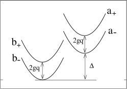
Figure 2: Schematic dispersion of a holon. b,a -corresponds to bonding and antibonding branches, and $\pm$ corresponds to the spiral splitting.

Populations of the four bands shown in Fig. 2 depend on the doping level $p$ and on the spiral wave vector $q$. When calculating energy, one has to remember that there are two planes. Therefore, the elastic energy per unit area is $2\times\rho_{s}q^{2}/2$, and the hole density per unit area is $2p$. It is convenient to define the following characteristic concentration

$$p_{0}=\frac{\Delta}{\pi\beta}\ .$$ (5)

A straighforward calculation shows that the dependences of the band filling and energy on doping $p$ and pitch $q$ are the following. Only the filled bands are noted below. In the case $p<p_{0}/2$ the both $b$-bands are filled at $q<\frac{\pi\beta}{g}p$ and at $q>\frac{\pi\beta}{g}p$ only the band $b_{-}$ is filled. The energy is

$$\frac{E}{\rho_{s}}=\left\{\begin{array}[]{ll}(1-\frac{\lambda}{2})q^{2}+\frac{\pi\beta}{\rho_{s}}p^{2}\ \ \ \ ,&q<\frac{\pi\beta}{g}p\\ q^{2}-2p\frac{g}{\rho_{s}}q+2\frac{\pi\beta}{\rho_{s}}p^{2}\ ,&q>\frac{\pi\beta}{g}p\end{array}\right.\quad.$$

In the case $p_{0}/2<p<p_{0}$ the bands $b_{\pm}$ are filled at $q<q_{1}$, the bands $b_{\pm}$ and $a_{-}$ are filled at $q_{1}<q<q_{2}$, and $b_{-}$, $a_{-}$ are filled at $q>q_{2}$. The energy reads

$$\frac{E}{\rho_{s}}=\left\{\begin{array}[]{lc}(1-\frac{\lambda}{2})q^{2}+\frac{\pi\beta}{\rho_{s}}p^{2}\ \ \ \ \ \ \ \ \ \ \ \ \ \ \ \ \ \ \ \ \ \ ,&q<q_{1}\\ \left(1-\frac{2}{3}\lambda\right)q^{2}+\frac{\lambda}{3}qq_{1}-\frac{\lambda}{6}q_{1}^{2}+\frac{\pi\beta}{\rho_{s}}p^{2}\ ,&q_{2}>q>q_{1}\\ q^{2}-2p\frac{g}{\rho_{s}}q+\frac{\pi\beta}{\rho_{s}}\left(p^{2}+pp_{0}-\frac{p_{0}^{2}}{4}\right)\ ,&q>q_{2}\end{array}\right.\quad.$$ (9)

In the case $p>p_{0}$ the bands $b_{\pm}$, $a_{\pm}$ are filled at $q<q_{3}$, the bands $b_{\pm}$ and $a_{-}$ are filled at $q_{3}<q<q_{2}$, and $b_{-}$, $a_{-}$ are filled at $q>q_{2}$. The energy reads

$$\frac{E}{\rho_{s}}=\left\{\begin{array}[]{lc}(1-\lambda)q^{2}+\frac{\pi\beta}{\rho_{s}}\left(\frac{p^{2}}{2}-\frac{p_{0}^{2}}{2}+pp_{0}\right)\ \ \ \ \ ,&q<q_{3}\\ \left(1-\frac{2}{3}\lambda\right)q^{2}-\frac{2\lambda}{3}qq_{3}-\frac{2\lambda}{3}q_{3}^{2}+\frac{\pi\beta}{\rho_{s}}p^{2}\ ,&q_{2}>q>q_{3}\\ q^{2}-2p\frac{g}{\rho_{s}}q+\frac{\pi\beta}{\rho_{s}}\left(p^{2}+pp_{0}-\frac{p_{0}^{2}}{4}\right)\ \ \ ,&q>q_{2}\end{array}\right.\quad.$$ (13)

In these formulas $q_{1}=\frac{\pi\beta}{g}(p_{0}-p)$,  $q_{2}=\frac{\pi\beta}{g}\left(\frac{p_{0}}{4}+\frac{p}{2}\right)$, and $q_{3}=\frac{\pi\beta}{g}\left(\frac{p}{2}-\frac{p_{0}}{2}\right)$.

The minimum of the energy with respect to $q$ gives the equilibrium spiral pitch $Q$ at a given doping level $p$. The result depends on $\lambda$. For $1<\lambda<\frac{3}{2}$ the pitch stays zero for $p<p_{0}$, then for $p_{0}<p<p_{1}$, where $p_{1}=0.5p_{0}/(\lambda-1)$, the pitch is

$$Q=\frac{g}{\rho_{s}}\frac{p-p_{0}}{3-2\lambda}\ ,$$ (14)

and finally at $p>p_{1}$ the pitch is given by the single layer formula (3). This behaviour is illustrated in Fig. 3(Left).

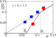
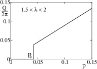
Figure 3: Incommensurate pitch versus doping.
Left: the regime $1<\lambda<1.5$. The solid line is the theory prediction for YBCO, the parameters are $\lambda=1.3$, $p_{0}=0.065$.
The dashed line is the theory prediction for LSCO. The red circles represent the YBCO neutron scattering data from Refs. hinkov07a ; hinkov07b ; hinkov04 . The blue squares represent the LSCO neutron scattering data from Ref. yamada98 .
Right: theoretical prediction for the pitch in the case $1.5<\lambda<2$.

In the case $\frac{3}{2}<\lambda<2$ the spin spiral pitch stays zero until the critical concentration $p_{c}=\frac{1}{\lambda}\left(1+\sqrt{1-\frac{\lambda}{2}}\right)p_{0}$, and then it jumps to the single layer value (3), see Fig. 3(Right). I would like to reiterate once more that the considered picture is valid for both the static and the dynamic spirals. Ultimately, the spiral always becomes dynamic at $p\geq 0.1-0.12$, see Ref. milstein07 . Clearly at $\frac{3}{2}<\lambda<2$ the jump at $p=p_{c}$ is the first order phase transition. On the other hand, $p_{0}$ and $p_{1}$ at $1<\lambda<\frac{3}{2}$ are Lifshitz points.

The value $\lambda\approx 1.3$ has been obtained from the fit of LSCO data milstein07 . The parameter $\lambda$ cannot be influenced by the relatively weak interlayer coupling, therefore the same value should be used for YBCO com . According to Refs. doiron ; miller the AF order in YBCO extends up to $p=0.06-0.07$, so let us take $p_{0}\approx 0.065$. This is another parameter of the theory. Having these two parameters one can predict the incommensurate wave vector in YBCO. The prediction is shown in Fig.3(Left) by the solid line The theory agrees very well with neutron scattering data shown by red circles hinkov07a ; hinkov07b ; hinkov04 . Using (5) one finds the value of the bonding-antibonding splitting, $\Delta\approx 70\mbox{meV}$. This is consistent with LDA calculations andersen95 and with ARPES data borisenko06 . In the same Fig.3(Left) the single layer theoretical $Q(p)$ is shown by the dashed line, and the neutron scattering LSCO data yamada98 are shown by the blue squares.

The developed theory is based on the small-$p$ expansion. Therefore, it is not surprising that at $p>0.12$ the experimental data start to deviate from the theory. Note also, that the single layer formula (3) is not applicable to LSCO at $p<0.055$. The region $p<0.055$ in LSCO corresponds to the strong localization regime and the relevant theory was developed in Ref. luscher07 .

The incommensurate spin ordering is a generic property of underdoped cuprates. However, the ordering properties and the phase diagrams of the single-layer LSCO and of the double-layer YBCO are remarkably different, see Fig. 1. It is shown that while in LSCO the intrinsic disorder to a large extent drives the magnetic properties, the role of disorder in YBCO is practically insignificant while the bilayer structure is crucial. The present analysis demonstrates also that the superconductivity is intimately related to the incommensurate spin ordering. In LSCO this relation is masked by the intrinsic disorder, superconductivity is impossible in the strongly-localized regime and therefore $p_{sc}$ is determined by percolation. However, in YBSO the correlation between superconductivity and incommensurate spin ordering is clear, the critical concentration for onset of superconductivity practically coincides with that for onset of the incommensurate spin order. Physical mechanisms behind this observation will be considered elsewhere.

I am grateful to O.K. Andersen and V. Hinkov for important discussions.

References

- (1) B. Keimer et al., Phys. Rev. B45, 7430 (1992).
- (2) Y. Ando, K. Segawa, S. Komiya, and A. N. Lavrov, Phys. Rev. Lett. 88, 137005 (2002).
- (3) X. F. Sun, K. Segawa, and Y. Ando, Phys. Rev. B 72, 100502R (2005).
- (4) N. Doiron-Leyraud et al., Phys. Rev. Lett. 97, 207001 (2006).
- (5) M. Matsuda et al., Phys. Rev. B65, 134515 (2002).
- (6) M. Fujita et al., Phys. Rev. B65, 064505 (2002).
- (7) K. Yamada et al., Phys. Rev. B57, 6165 (1998).
- (8) R. I. Miller et al., Phys. Rev. B 73, 144509 (2006).
- (9) V. Hinkov et al., Nature Physics 3, 780 (2007).
- (10) V. Hinkov et al., Science 319, 597 (2008).
- (11) V. Hinkov et al., Nature 430, 650 (2004).
- (12) O. P. Sushkov and V. N. Kotov, Phys. Rev. Lett. 94, 097005 (2005).
- (13) A. Lüscher, G. Misguich, A. I. Milstein, and O. P. Sushkov, Phys. Rev. B73, 085122 (2006).
- (14) A. Lüscher, A. I. Milstein, and O. P. Sushkov, Phys. Rev. Lett. 98, 037001 (2007).
- (15) B. I. Shraiman and E. D. Siggia, Phys. Rev. Lett. 61, 467 (1988); Phys. Rev. Lett. 62, 1564 (1989); Phys. Rev. B42, 2485 (1990).
- (16) A. I. Milstein and O. P. Sushkov, Phys. Rev. B78, 014501 (2008).
- (17) R. R. P. Singh, Phys. Rev. B 39, 9760 (1989); Zheng Weihong, J. Oitmaa, and C. J. Hamer, Phys. Rev B 43, 8321 (1991).
-
(18)
D. Reznik et al.,
Phys. Rev. B53, R14741 (1996);
S. M. Hayden et al., Phys. Rev. B54, R6905 (1996). - (19) O. K. Andersen, A. I. Liechtenstein, O. Jepsen, and F. Paulsen, J. Phys. Chem. Solids 56, 1573 (1995).
- (20) S. V. Borisenko et al., Phys. Rev. Lett. 96, 117004 (2006).
- (21) The hopping matrix elements and in YBCO are slightly different from that in LSCO. This can give a small difference in the value of .