Characterization of integrated optics components for the second generation of VLTI instruments

Abstract

Two of the three instruments proposed to ESO for the second generation instrumentation of the VLTI would use integrated optics for beam combination. Several design are studied, including co-axial and multi-axial recombination. An extensive quantity of combiners are therefore under test in our laboratories. We will present the various components, and the method used to validate and compare the different combiners. Finally, we will discuss the performances and their implication for both VSI and Gravity VLTI instruments.

1 INTRODUCTION

To pursue the development and increase the capabilities of the VLTI, ESO selected three instrumental projects in phase A. The three new instruments are : MATISSE, VSI, and GRAVITY. MATISSE is a mid-infrared spectro-interferometer. VSI and GRAVITY are two near-infrared instruments, both with the specificity of using integrated optics beam combiners [1, 2, 3, 4, 5, 6]. To that end, new integrated optics (IO) beam combiners were developed. The requirements for VSI were:

• Being able to work in the J, H and K band.

• Being able to combine up to 6 telescopes.

on the other hand, GRAVITY had several criterium to meet:

• High sensitivity in the K band (more than 50% throughput for the beam combiner as a whole).

• Non-temporal modulation to allow long integration time exposures.

The basic concept for the combiner was an ABCD type-recombination [7]. Such a combiner was already presented by M. Benisty et al. [8]. Multi-axial 6 beam combiners component are also investigated as a good alternative. The goal of this new development round is to: (i) prove the validity of the technology for the K and J band, and (ii) improve the throughput and therefore the sensitivity by testing different arrangement of the waveguide paths. Several new combiners were therefore designed, and were recently delivered to our laboratory.

2 THE WAFER

CEA/LETI technical processes use Silica on Silicum, and a lithographic technique for waveguide tracing. Figure 1 gives an overview of the photomask which was used to transfer the waveguide paths on the wafer. On this mask, there are 48 beam combiners. Each type of combiner is duplicated on the right and the left of the wafer. Each combiner also comes in three versions, corresponding to guides of different size. For example, the H band combiners exist with guides of 6.8$\,\mu$m 7$\,\mu$m and 7.2$\,\mu$m. The size of the wafer is $8\times 8$ inches.

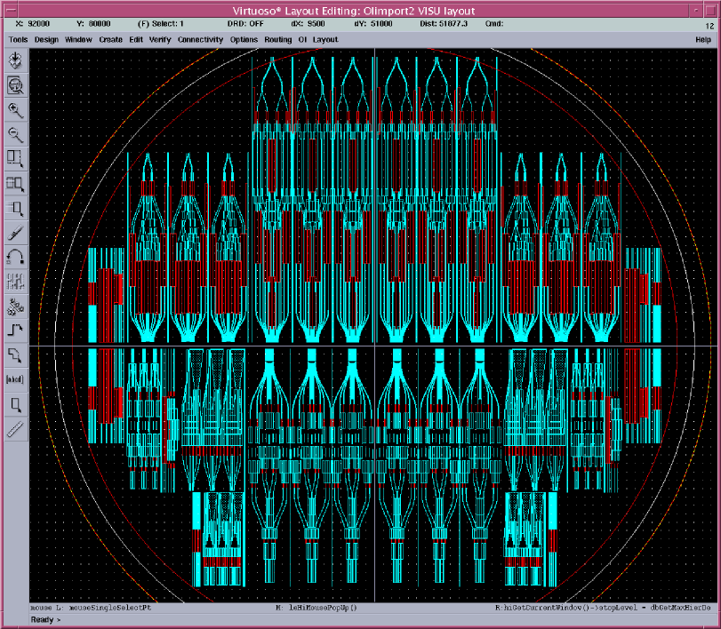
Figure 1: Overview of the wafer guide tracing. On this $8\times 8$ inches wafer are 48 beam combiners.

The new types of combiners are:

• A 4 telescopes ABCD beam combiner in the H band. The goal of this combiner is to test new achromatized phase shifts. This to (i) increase the contrast ratio at the output by compensating the chromatic effects of the couplers, and (ii) increase the precision on the closure phases by having them constant over a large bandpass.

• A second 4 telescopes ABCD beam combiner in H band. The size of the beam combiner is reduced by 30% by using a combination of 66/33% and 50/50% couplers instead of a tricoupler. The component is therefore not symmetric anymore, with an eventual effect on the closure phase.

• Two 2 telescopes ABCD beam combiners to test transmission and response of the K and J band.

• A 4 telescopes ABCD fringe tracking combiner in the K band. Since only pistons measurements are needed, such a combiner combine the flux using “bootstrapping” approach (ie., each telescope is recombined with two other telescopes only). The goal for this component is to validate fringe tracker algorithms with an ABCD combiner.

• Two 6 telescopes multi-axial beam combiners, working in K and H bands

3 CHARACTERIZATION I. TRANSMISSION

Throughput was investigated by the means of two single mode fibers. One is used to inject the light in the component, and the other to convey the flux from the outputs of the component to a K band monopixel detector. The flux recorded on all the outputs is then summed, and normalized by the flux measured when putting the two single mode fibers in contact with each other. Errors are of the order of half a percent.

Table 1: Transmission of the 2 telescopes ABCD beam combiner in the K band.

Wavelength	Guide width	Input 1	Input 2
$2.20\,\mu$m	$9.8\,\mu$m	52.0 %	52.5 %
$2.20\,\mu$m	$10.0\,\mu$m	51.9 %	53.4 %
$2.20\,\mu$m	$10.2\,\mu$m	60.0 %	53.0 %
$2.37\,\mu$m	$9.8\,\mu$m	65.8 %	66.2 %
$2.37\,\mu$m	$10.0\,\mu$m	68.4 %	67.9 %
$2.37\,\mu$m	$10.2\,\mu$m	67.6 %	68.9 %

Tests were performed on the K band ABCD using two different SLED: one at 2.2$\,\mu$m, and one at 2.37$\,\mu$m. Results are reported in Table 1. The 50% transmission goal was achieved at both wavelength. Optimization of the waveguide paths could eventually further increase the transmission.

4 CHARACTERIZATION II. COHERENT TRANSFER FUNCTION

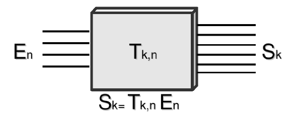
Figure 2: Generalization of the transfer function of an integrated optics device. $n$ are inputs, $k$ outputs. $E_{k}$ and $S^{k}$ are respectively the entering and exiting complex electric field.

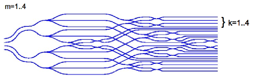
Figure 3:

Figure 2 represents the generalized view of the transfer function of an integrated optic component. $E_{n}$ is the complex electric field entering the component via input $n$, and $S^{k}$ is the resulting field on output number $k$. $T_{n}^{k}$ is a two dimensional complex matrix linking $S^{k}$ to $E_{n}$.

A complete determination of the transfer function of the IO would therefore be equivalent to the determination of matrix $T_{n}^{k}$. However, the observable is not $S^{k}$ , but the intensity on the output channels:

$$|S^{k}|^{2} = \left|\sum_{n}T_{n}^{k}E_{n}\right|^{2}$$ (1)

$$= \Re\left[\sum_{n}|T_{n}^{k}E_{n}|^{2}+2\sum_{n}\sum_{m>n}T_{n}^{k}T_{m}^{k*}\ E_{n}E_{m}\right]\,.$$ (2)

However, this equation assume a fully coherent incoming beam, and no loss of contrast due to, for example, chromaticity, polarization etc… Hence, we introduced two extra terms: $V_{n,m}$ correspond to the coherency of the incoming electric field (the complex visibility). $C_{n,m}^{k}$ correspond to the level of which the IO device conserve the coherence of the light:

$$|S^{k}|^{2}=\Re\left[\sum_{n}|T_{n}^{k}E_{n}|^{2}+2\sum_{n}\sum_{m>n}T_{n}^{k}T_{m}^{k*}C_{n,m}^{k}\ E_{n}E_{m}^{*}V_{n,m}\right]\,.$$ (3)

Equation (3) can be rewritten with a matrix product:

$$\left(\begin{array}[]{c}|S^{1}|^{2}\\ \vdots\\ |S^{K}|^{2}\end{array}\right)=\Re\left[V2PM\cdot\left(\begin{array}[]{c}|E_{1}|^{2}\\ \vdots\\ |E_{N}|^{2}\\ E_{1}E_{2}^{*}V_{1,2}\\ \vdots\\ E_{N-1}E_{N}^{*}V_{N-1,N}\\ \end{array}\right)\right]$$ (4)

where $N$ is the total number of inputs, and $K$ the number of outputs. The $V2PM$ matrix is then equal to:

$$V2PM=\left(\begin{array}[]{cccccc}|T_{1}^{1}|^{2}&\cdots&|T_{N}^{1}|^{2}&2T_{1}^{1}T_{2}^{1*}C_{1,2}^{1}&\cdots&2T_{N-1}^{1}T_{N}^{1*}C_{N-1,N}^{1}\\ \vdots&&\vdots&\vdots&&\vdots\\ |T_{1}^{K}|^{2}&\cdots&|T_{N}^{K}|^{2}&2T_{1}^{K}T_{2}^{K*}C_{1,2}^{K}&\cdots&2T_{N-1}^{K}T_{N}^{K*}C_{N-1,N}^{K}\end{array}\right)$$ (5)

The name $V2PM$ was adopted in accordance with previous data reduction done on multi-axial interferometers[9]. It stands for “Visibilities to Pixels Matrix”.

Characterization of the components will consist in the determination of the V2PM. Providing a well engineered OI, the V22M shall be invertible, allowing a robust determination of the photometry channels ($|E_{n}|^{2}$), as well as the contrasts and phases ($E_{n}E_{m}^{*}V_{n,m}$).

We tested the method on the OI combiner already discussed by Benisty et al.[8]. The schematic of the combiner is reproduced figure 3. In the ideal case, the V2PM would wrote :

$$V2PM=\left(\begin{array}[]{cccccccccc}\frac{1}{12}&\frac{1}{12}&0&0&\frac{1}{6}&0&0&0&0&0\\ \frac{1}{12}&\frac{1}{12}&0&0&\frac{1}{6}e^{i\pi}&0&0&0&0&0\\ \frac{1}{12}&\frac{1}{12}&0&0&\frac{1}{6}e^{i\pi/2}&0&0&0&0&0\\ \frac{1}{12}&\frac{1}{12}&0&0&\frac{1}{6}e^{i3\pi/2}&0&0&0&0&0\\ 0&\frac{1}{12}&\frac{1}{12}&0&0&\frac{1}{6}&0&0&0&0\\ 0&\frac{1}{12}&\frac{1}{12}&0&0&\frac{1}{6}e^{i\pi}&0&0&0&0\\ \frac{1}{12}&0&\frac{1}{12}&0&0&0&0&0&0&\frac{1}{6}\\ \frac{1}{12}&0&\frac{1}{12}&0&0&0&0&0&0&\frac{1}{6}e^{i\pi}\\ \frac{1}{12}&0&\frac{1}{12}&0&0&0&0&0&0&\frac{1}{6}e^{i\pi/2}\\ \frac{1}{12}&0&\frac{1}{12}&0&0&0&0&0&0&\frac{1}{6}e^{i3\pi/2}\\ \frac{1}{12}&0&0&\frac{1}{12}&0&0&0&\frac{1}{6}&0&0\\ \frac{1}{12}&0&0&\frac{1}{12}&0&0&0&\frac{1}{6}e^{i\pi}&0&0\\ \frac{1}{12}&0&0&\frac{1}{12}&0&0&0&\frac{1}{6}e^{i\pi/2}&0&0\\ \frac{1}{12}&0&0&\frac{1}{12}&0&0&0&\frac{1}{6}e^{i3\pi/2}&0&0\\ 0&\frac{1}{12}&0&\frac{1}{12}&0&0&\frac{1}{6}&0&0&0\\ 0&\frac{1}{12}&0&\frac{1}{12}&0&0&\frac{1}{6}e^{i\pi}&0&0&0\\ 0&\frac{1}{12}&0&\frac{1}{12}&0&0&\frac{1}{6}e^{i\pi/2}&0&0&0\\ 0&\frac{1}{12}&0&\frac{1}{12}&0&0&\frac{1}{6}e^{i3\pi/2}&0&0&0\\ 0&\frac{1}{12}&\frac{1}{12}&0&0&\frac{1}{6}e^{i\pi/2}&0&0&0&0\\ 0&\frac{1}{12}&\frac{1}{12}&0&0&\frac{1}{6}e^{i3\pi/2}&0&0&0&0\\ 0&0&\frac{1}{12}&\frac{1}{12}&0&0&0&0&\frac{1}{6}&0\\ 0&0&\frac{1}{12}&\frac{1}{12}&0&0&0&0&\frac{1}{6}e^{i\pi}&0\\ 0&0&\frac{1}{12}&\frac{1}{12}&0&0&0&0&\frac{1}{6}e^{i\pi/2}&0\\ 0&0&\frac{1}{12}&\frac{1}{12}&0&0&0&0&\frac{1}{6}e^{i3\pi/2}&0\end{array}\right)$$ (6)

There are several ways to obtained the matrix of “real”combiner. We used a method which determine the matrix column by column. The first four columns correspond to the real transmission of each one of the entrance separately. To determine these four columns, we inject light into the entrance guides one after the other. For the six following column, light is injected into two entrances only, and optical path modulated to reveals the phase shifts.

On one of our 4T ABCD H band beam combiner, we obtained the following matrix:

$${V2PM=\left(\begin{array}[]{rrrrrrrrrr}0.085&0.039&0.001&0.001&0.112e^{0.00i}&0.000e^{-2.02i}&0.000e^{0.21i}&0.001e^{-2.04i}&0.000e^{2.79i}&0.000e^{2.51i}\\ 0.037&0.065&0.001&0.001&0.099e^{3.13i}&0.001e^{1.25i}&0.000e^{-1.65i}&0.000e^{-0.52i}&0.000e^{0.55i}&0.000e^{-2.79i}\\ 0.045&0.022&0.001&0.001&0.063e^{1.25i}&0.000e^{-0.80i}&0.000e^{-0.36i}&0.000e^{1.24i}&0.000e^{0.95i}&0.000e^{-2.46i}\\ 0.041&0.074&0.001&0.001&0.108e^{-1.88i}&0.001e^{0.53i}&0.000e^{2.82i}&0.000e^{1.84i}&0.000e^{-0.54i}&0.001e^{2.28i}\\ 0.002&0.067&0.054&0.002&0.002e^{2.27i}&0.116e^{-0.00i}&0.001e^{-3.11i}&0.001e^{-2.01i}&0.002e^{2.63i}&0.001e^{-0.43i}\\ 0.003&0.051&0.077&0.003&0.002e^{-1.03i}&0.121e^{3.14i}&0.001e^{2.40i}&0.001e^{0.71i}&0.000e^{1.28i}&0.003e^{3.08i}\\ 0.206&0.000&0.089&0.002&0.001e^{-0.09i}&0.002e^{0.43i}&0.000e^{-2.03i}&0.002e^{-0.04i}&0.001e^{2.79i}&0.261e^{0.00i}\\ 0.098&0.002&0.173&0.001&0.000e^{-2.84i}&0.001e^{1.24i}&0.000e^{2.99i}&0.001e^{0.31i}&0.001e^{0.19i}&0.256e^{3.14i}\\ 0.192&0.002&0.095&0.002&0.001e^{0.29i}&0.002e^{2.23i}&0.000e^{-2.10i}&0.002e^{-2.92i}&0.003e^{-0.99i}&0.263e^{0.97i}\\ 0.078&0.002&0.146&0.002&0.001e^{-1.19i}&0.001e^{2.69i}&0.000e^{2.71i}&0.002e^{-0.09i}&0.002e^{-1.57i}&0.213e^{-2.16i}\\ 0.093&0.003&0.000&0.035&0.001e^{-1.08i}&0.001e^{2.44i}&0.002e^{1.64i}&0.107e^{-0.00i}&0.001e^{-2.99i}&0.004e^{0.88i}\\ 0.044&0.004&0.004&0.101&0.001e^{2.30i}&0.002e^{-2.90i}&0.001e^{-1.75i}&0.127e^{3.13i}&0.002e^{-1.89i}&0.001e^{1.40i}\\ 0.037&0.003&0.003&0.014&0.001e^{2.59i}&0.001e^{1.32i}&0.000e^{1.36i}&0.042e^{0.94i}&0.001e^{-2.05i}&0.001e^{2.74i}\\ 0.020&0.002&0.002&0.043&0.001e^{-2.59i}&0.000e^{2.44i}&0.001e^{-0.86i}&0.054e^{-2.15i}&0.000e^{2.10i}&0.001e^{-1.80i}\\ 0.002&0.178&0.003&0.095&0.001e^{0.07i}&0.001e^{-2.40i}&0.237e^{0.00i}&0.000e^{-1.37i}&0.001e^{3.12i}&0.001e^{-2.57i}\\ 0.002&0.094&0.002&0.188&0.001e^{2.41i}&0.001e^{1.62i}&0.251e^{3.13i}&0.001e^{-1.89i}&0.001e^{-0.44i}&0.000e^{-0.85i}\\ 0.002&0.173&0.002&0.097&0.001e^{0.12i}&0.001e^{0.75i}&0.246e^{1.20i}&0.001e^{-0.27i}&0.001e^{-0.81i}&0.001e^{1.86i}\\ 0.002&0.089&0.002&0.187&0.000e^{-0.41i}&0.000e^{-0.41i}&0.245e^{-1.94i}&0.001e^{-2.21i}&0.000e^{-1.93i}&0.001e^{-2.92i}\\ 0.003&0.075&0.049&0.001&0.002e^{-2.88i}&0.113e^{1.35i}&0.003e^{1.60i}&0.002e^{-1.19i}&0.000e^{2.80i}&0.002e^{-1.19i}\\ 0.002&0.051&0.071&0.003&0.002e^{-1.16i}&0.112e^{-1.77i}&0.004e^{-2.65i}&0.001e^{2.21i}&0.004e^{1.99i}&0.002e^{2.57i}\\ 0.002&0.001&0.083&0.041&0.001e^{1.30i}&0.001e^{1.68i}&0.000e^{-2.87i}&0.000e^{-0.59i}&0.108e^{0.00i}&0.001e^{-2.69i}\\ 0.001&0.002&0.041&0.079&0.001e^{0.56i}&0.001e^{1.52i}&0.001e^{1.93i}&0.001e^{2.17i}&0.109e^{-3.14i}&0.000e^{-1.67i}\\ 0.001&0.001&0.068&0.036&0.000e^{-2.51i}&0.000e^{2.92i}&0.000e^{1.81i}&0.001e^{-1.47i}&0.094e^{1.26i}&0.000e^{2.85i}\\ 0.001&0.001&0.033&0.066&0.000e^{-2.86i}&0.000e^{-0.14i}&0.000e^{-2.12i}&0.000e^{-0.01i}&0.090e^{-1.86i}&0.000e^{2.40i}\\ \end{array}\right)}$$ (7)

The differences between matrix (5) and (6) are due several instrumental effects. These effects are revealed by :

• Missing zero values in the first four columns. This is due to crosstalk, consequence of some flux going from one guide to another because of, for example, intersections. In column 1, the crosstalk is of the order of 1%.

• Values different from $\frac{1}{12}$ in the first four columns. This due to a transmission not perfectly equilibrated between the different channels after a coupler or a tricoupler.

• Phase shifts different than $[0,\pi,\pi/2,3\pi/2]$ for the four main outputs of each telescope pairs. This is a problem due to the engineering of the phase shift.

5 CONCLUSION

OI circuits presented in Figure 1 have recently been delivered to our laboratory. We have shown that the transmission of the components is adapted for astronomical observations in the K band. Optimization of the throughput is nevertheless still under investigation, with possibilities offered by using new couplers, optical paths, and/or fiber to combiner injection methods.

We also developed the tools to fully characterize the complex transfer function of the new components, to have rigorous comparison between the different combiner engineered. The knowledge of the $V2PM$ matrix should also allow signal to noise estimation, to provide sound and practical way to choose the best combiner for the VLTI.

References

[1]
Malbet, F., Kern, P., Schanen-Duport, I., Berger, J.-P.,
Rousselet-Perraut, K., and Benech, P., “Integrated optics for
astronomical interferometry. I. Concept and astronomical applications,”
A&AS 138, 135–145 (July 1999).
[2]
Berger, J. P., Rousselet-Perraut, K., Kern, P., Malbet, F.,
Schanen-Duport, I., Reynaud, F., Haguenauer, P., and Benech, P.,
“Integrated optics for astronomical interferometry. II. First laboratory
white-light interferograms,” A&AS 139, 173–177 (Oct. 1999).
[3]
Haguenauer, P., Berger, J.-P., Rousselet-Perraut, K., Kern, P.,
Malbet, F., Schanen-Duport, I., and Benech, P., “Integrated Optics
for Astronomical Interferometry. III. Optical Validation of a Planar Optics
Two-Telescope Beam Combiner,” Appl. Opt. 39, 2130–2139 (May 2000).
[4]
Berger, J. P., Haguenauer, P., Kern, P., Perraut, K., Malbet, F.,
Schanen, I., Severi, M., Millan-Gabet, R., and Traub, W.,
“Integrated optics for astronomical interferometry. IV. First measurements
of stars,” A&A 376, L31–L34 (Sept. 2001).
[5]
Laurent, E., Rousselet-Perraut, K., Benech, P., Berger, J. P., Gluck,
S., Haguenauer, P., Kern, P., Malbet, F., and Schanen-Duport, I.,
“Integrated optics for astronomical interferometry. V. Extension to the K
band,” A&A 390, 1171–1176 (Aug. 2002).
[6]
Lebouquin, J.-B., Labeye, P., Malbet, F., Jocou, L., Zabihian, F.,
Rousselet-Perraut, K., Berger, J.-P., Delboulbé, A., Kern, P.,
Glindemann, A., and Schöller, M., “Integrated optics for
astronomical interferometry. VI. Coupling the light of the VLTI in K band,”
A&A 450, 1259–1264 (May 2006).
[7]
Shao, M. and Staelin, D. H., “Long-baseline optical interferometer for
astrometry,” Journal of the Optical Society of America
(1917-1983)67, 81–86 (Jan. 1977).
[8]
Benisty, M., Berger, J.-P., Jocou, L., Malbet, F., Perraut, K.,
Labeye, P., and Kern, P., “The VSI/VITRUV combiner: a phase-shifted
four-beam integrated optics combiner,” in [Advances in Stellar
Interferometry. Edited by Monnier, John D.; Schöller, Markus; Danchi,
William C.. Proceedings of the SPIE, Volume 6268, pp. 62682D
(2006). ], Presented at the Society of
Photo-Optical Instrumentation Engineers (SPIE) Conference6268 (July
2006).
[9]
Tatulli, E. and LeBouquin, J.-B., “Comparison of Fourier and model-based
estimators in single-mode multi-axial interferometry,” MNRAS 368, 1159–1168 (May 2006).