On the incidence-prevalence relation and length-biased sampling

Abstract.

For many diseases, logistic and other constraints often render large incidence studies difficult, if not impossible, to carry out. This becomes a drawback, particularly when a new incidence study is needed each time the disease incidence rate is investigated in a different population. However, by carrying out a prevalent cohort study with follow-up it is possible to estimate the incidence rate if it is constant. In this paper we derive the maximum likelihood estimator (MLE) of the overall incidence rate, $\lambda$, as well as age-specific incidence rates, by exploiting the well known epidemiologic relationship, prevalence = incidence $\times$ mean duration ($P=\lambda\times\mu$). We establish the asymptotic distributions of the MLEs, provide approximate confidence intervals for the parameters, and point out that the MLE of $\lambda$ is asymptotically most efficient. Moreover, the MLE of $\lambda$ is the natural estimator obtained by substituting the marginal maximum likelihood estimators for P and $\mu$, respectively, in the expression $P=\lambda\times\mu$. Our work is related to that of Keiding (1991, 2006), who, using a Markov process model, proposed estimators for the incidence rate from a prevalent cohort study without follow-up, under three different scenarios. However, each scenario requires assumptions that are both disease specific and depend on the availability of epidemiologic data at the population level. With follow-up, we are able to remove these restrictions, and our results apply in a wide range of circumstances. We apply our methods to data collected as part of the Canadian Study of Health and Ageing to estimate the incidence rate of dementia amongst elderly Canadians.

1. Introduction

In an incidence study, whose goal is to estimate a disease incidence rate, a cohort of initially disease-free subjects is followed forward in time. The subjects are monitored closely and for those who develop the disease their approximate times of disease onset are recorded. Often, as part of an incidence study, these diseased subjects are followed until “failure” or censoring. The data collected from such an incidence study may then be used to directly estimate both the disease incidence rate and the survival function for the time from onset to failure. The estimators of the incidence rate and the survival function from such data are standard.

For many diseases, however, logistic and other constraints often render large incidence studies difficult, if not impossible, to carry out. This becomes a drawback, particularly when a new incidence study is needed each time the disease incidence rate is investigated in a different population. Nevertheless, by carrying out a prevalent cohort study with follow-up it is possible to estimate the incidence rate if it is constant, thus avoiding the problems associated with incidence studies. In this paper we derive the maximum likelihood estimator (MLE) of the overall incidence rate, $\lambda$, as well as age-specific incidence rates from data collected as part of a prevalent cohort study with follow-up. We exploit the well known epidemiologic relationship, prevalence = incidence $\times$ mean duration ($P=\lambda\times\mu$), to suggest that the likelihood be derived as a function of the vector ($P$, $\mu$). Once the MLE, $(\hat{P},\hat{\mu})$ of $(P,\mu)$, is obtained, the MLE of $\lambda=\frac{P}{\mu}$ follows by invariance. A similar approach may be used to find the MLEs of age specific incidence rates. The asymptotic distributional properties of the estimators may be obtained by modifying previous results for the MLE of the survival function, based on survival data from a prevalent cohort study with follow-up (see Section 4). It is comforting that the MLE $\hat{\lambda}=\frac{\hat{P}}{\hat{\mu}}$ is, therefore, also the natural ad hoc estimator of $\lambda$.

In a medical setting, a prevalent cohort study with follow-up (Wang 1991) begins with the identification, from a sampled cohort, of those with existing (prevalent) disease. The dates of onset for the diseased are ascertained and the diseased subjects are followed forward in time until failure or censoring. Other data collected include the ages at the time of recruitment, the failure/censoring times of the subjects who are followed, and covariates of interest to the researchers. There are two main features of the data collected from such studies. First, the dates of disease onset of the prevalent cases do not include the dates of onset of those who died prior to the start of the prevalent cohort study; we can only speculate as to the existence of such subjects. Hence, direct use of the observed dates of onset from a prevalence study, in contrast to dates of onset from an incidence study, leads to underestimation of the true incidence rate. Second, the observed failure/censoring intervals are left-truncated and, if the underlying incidence process is stationary, as is the assumption here, they are length biased; those with longer survival intervals are more likely to be observed (Wicksell 1925, Neyman 1955, Cox 1969, Patil and Rao 1978, and Vardi 1982, 1985). We address these difficulties in deriving the MLE ($\hat{P},\hat{\mu}$) and hence the MLE $\hat{\lambda}$, of the overall incidence rate. We use a similar approach to the estimation of age-specific incidence rates.

Keiding (1991, 2006) used a Markov process model to derive carefully, the prevalence-incidence relationship, and proposed three different scenarios which facilitate estimation of the (constant) age-specific incidence rate when there are no follow-up data. In the first scenario it is assumed that there is non-differential mortality for the diseased and non-diseased. In Biering-Sorensen and Hilden (1984) this assumption is likely to be tenable while in Keiding et al. (1989), it is probably not, since the disease under study is diabetes. In the second scenario, which Keiding invokes in his 1989 paper, no assumption of non-differential mortality is made. It is either assumed that the incidence rate is small and that the difference between the intensities from the healthy and diseased states to death is known or that the difference between these two intensities is small and known. In the third scenario, it is assumed that the joint relative intensity of the calendar time, age- and duration-specific mortality is known. Under each scenario a parametric assumption must be made, and in the last two scenarios certain population parameters must be known. Therefore, these estimators are strongly disease-specific and also dependent on the availability of certain population level data. These assumptions are needed to compensate for not having follow-up information. By following-up the prevalent cases we are able to avoid these assumptions. Our main assumption is that the underlying incidence process is a stationary Poisson process, an assumption that Keiding also makes. Stationarity of the incidence rate holds, roughly, for many diseases: for example, amyotrophic lateral sclerosis (Sorenson et al. 2002), certain types of cancers (Jemal et al. 2005), and schizophrenia (Folnegovic and Folnegovic-Smalc 1992). It may not, however, be tenable for an infectious disease.

Diamond and McDonald (1991) also considered incidence rate estimation from prevalent-case data, with no follow-up, again under different assumptions. Ogata et al. (2000) took an empirical Bayes approach to the analysis of retrospective incidence data. More recently Alioum et al. (2005) make HIV-AIDS-specific model assumptions to estimate a general incidence rate. To our knowledge there is no literature that provides a general framework for maximum likelihood estimation of a constant underlying incidence rate when one has access only to prevalent cohort survival data with follow-up.

The rest of this paper is organized as follows: In Section 2 we provide a careful formulation of a prevalent cohort study with follow-up, paying particular attention to survival data. In Section 3 we discuss the MLE for the underlying incidence rate. In Section 4, we present the asymptotic properties of the estimator, paving the way for computation of an approximate confidence interval for the underlying incidence rate. In Section 5 we extend our results to include age-specific incidence rates. In Section 6 we apply our methods to data collected as part of the Canadian Study of Health and Aging (CSHA), in order to estimate the underlying age-specific incidence rates of dementia amongst the elderly in Canada.

2. General setup and notation

Let $X_{1},X_{2},...,X_{m}$ be $m$ i.i.d. positive random variables representing the survival times of individuals from onset of a disease, say, to an end point of interest. Let the $X_{i}$’s have survivor function $S(x)=P(X_{i}>x)$, cumulative distribution function $F(x)$, and probability density function $f(x)$. Define $\mu$ to be the mean survival time; that is, $\mu=\int_{0}^{\infty}S(x)dx$. Suppose that $\tau_{1},\tau_{2},...,\tau_{m}$ are the $m$ calendar times of onset corresponding to $X_{1},X_{2},...,X_{m}$ and let $\tau^{*}$ be the calendar time of recruitment into a study. Individual $i$ is observed in the study only if $X_{i}\geq\tau^{*}-\tau_{i}$ and, therefore, for $i=1,2,...,m$, $X_{i}$ is left truncated with left truncation time $T_{i}=\tau^{*}-\tau_{i}$. Since the onset times are random, the truncation times are random variables, with distribution function denoted by $G$, and density $g$. Let $Y_{1},Y_{2},...,Y_{n}$ be the observed left truncated lifetimes, with $n\leq m$. That is, $P(Y_{i}>x)=P(X_{i}>x|X_{i}>T_{i})$. We borrow terminology from renewal theory and write $Y_{i}=Y_{i}^{bwd}+Y_{i}^{fwd}$, where $Y_{i}^{bwd}$ is the time from onset to recruitment into the study or the “backward recurrence time”, and $Y_{i}^{fwd}$ is the time from recruitment to failure, or the “forward recurrence time”. Also, let $F_{LB}$ represent the distribution of the $Y_{i}$’s, where the subscript, $LB$, is used to indicate that the $Y_{i}$’s are length-biased.

Suppose that individual $i$ has censoring time $C_{i}^{*}=Y_{i}^{bwd}+C_{i}$, where $C_{i}$, which we call the “residual censoring time”, is the time from recruitment until the individual is censored. We assume that P($C_{i}^{*}>T_{i}$) = 1 (see Wang 1991) and we thus observe only $\min(C_{i}^{*},Y_{i})$. Often, however, the backward recurrence times are fully observed, and we assume this to be the case here, so that the observed data are: $(Y_{i}^{bwd},Y_{i}^{obs},\delta_{i})\ i=1,2,...,n$ where $Y_{i}^{obs}=min(Y_{i}^{fwd},C_{i})$ and $\delta_{i}=I[Y_{i}^{fwd}\leq C_{i}]$ indicates whether subject $i$ has been followed until failure. Since $C_{i}^{*}$ and $Y_{i}$ share $Y_{i}^{bwd}$, the full survival times, $Y_{i}$, are informatively censored (Vardi 1989). It is still reasonable in many cases, however, to assume that $C_{i}$ is independent of both $Y_{i}^{fwd}$ and $Y_{i}^{bwd}$, since independence between $C_{i}$ and $Y_{i}^{fwd}$ corresponds to the usual random censoring assumption.

In summary, we differentiate between the potential failure times, $X_{i}$, some of which will not be observed because of left truncation, and the observed failure/censoring times ($Y_{i}^{bwd}$ + $Y_{i}^{obs}$); these are event times of the “long survivors”.

3. Point estimation of the incidence rate

Under stationarity we assume the underlying incidence process is a Poisson process with constant intensity $\lambda(t)\equiv\lambda$. Hence, the truncation time distribution, $G$, is uniform, conditional on the number of incident times in $(0,\tau^{*})$ (Asgharian, Wolfson, and Zhang 2006).

We begin by deriving the MLE of $\lambda$. We then derive the MLE of the age-specific incidence rates. The approach depends on the well-known relationship, $P=\lambda\times\mu$ where $P$ is the time-independent point prevalence, $\lambda$ is the time-independent underlying incidence rate, and $\mu$ is the mean duration of the disease (see Keiding 1991).

Let a random number of $N$ prevalent cases be observed from a large group of $s$ individuals selected from screening. Fixing $N$ at $n$, the realized number of prevalent cases, Asgharian, M’Lan, and Wolfson (2002) and Asgharian and Wolfson (2005) derived the unconditional NPMLE, $\hat{S}$, of $S$ under the assumption of stationarity. They established its asymptotic properties and those of the NPMLE, $\hat{\mu}=\int_{0}^{\infty}\hat{S}(x)dx$. Conditioning on $N=n$, the likelihood of the data is

(1) $$L=L(S,P)=f(\text{data},n;S,P).$$

Write $L(S,P)$ as $L(S|n)L(P)=f(\text{data};S|n)f(n;P)$, by sufficiency of $N$ for $P$. Now, in practice, the data of a prevalent cohort study with follow-up are collected in two stages. In stage 1, a binary, 0-1, random variable, say $\xi$, is measured on each randomly selected subject to ascertain if the subject has experienced initiation of the disease. In stage 2, we observe the triple $(Y_{i}^{bwd},Y_{i}^{obs},\delta_{i})\ i=1,2,...,n$ on diseased subjects, indicated by $\xi=1$. The following tree diagram depicts our sampling scheme:

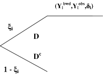
Figure 1. Sampling scheme

The full likelihood is:

(2) $$L=\prod_{i=1}^{s}(1-P)^{1-\xi_{i}}\Bigg{[}P\Bigg{(}\frac{dF(y_{i}^{bwd}+y_{i}^{fwd})}{\mu}\Bigg{)}^{\delta_{i}}\Bigg{(}\int_{\omega\geq y_{i}^{bwd}+c_{i}}\frac{dF(\omega)}{\mu}\Bigg{)}^{1-\delta_{i}}\Bigg{]}^{\xi_{i}},$$

where $P=P(\xi=1)$ is the time-independent point prevalence in the population. For the derivation of a similar likelihood see Asgharian and Wolfson (2005). As is readily seen, the above likelihood can be factorized as

(3) $$L=\Bigg{[}\prod_{i=1}^{s}(1-P)^{1-\xi_{i}}P^{\xi_{i}}\Bigg{]}\ \Bigg{[}\prod_{i=1}^{s}\Bigg{(}\frac{dF(y_{i}^{bwd}+y_{i}^{fwd})}{\mu}\Bigg{)}^{\delta_{i}}\Bigg{(}\int_{\omega\geq y_{i}^{bwd}+c_{i}}\frac{dF(\omega)}{\mu}\Bigg{)}^{1-\delta_{i}}\Bigg{]}^{\xi_{i}}\\$$

Joint maximization of (2) with respect to $S$ and $P$ gives the NPMLE $(\hat{S},\hat{P})$ and hence the NPMLE $(\hat{\mu},\hat{P})$ where $\hat{P}=N/s$ is the usual point prevalence estimator of $P$. It follows, by invariance, that $\hat{\lambda}=\hat{P}/\hat{\mu}$ is the unconditional NPMLE of $\lambda$. It is seen that $\hat{\lambda}$, the MLE, is also the natural ad hoc estimator derived from the relation $\lambda=P/\mu$, by replacing $P$ and $\mu$ by their respective natural estimators.

Wang (1991) derived the NPMLE $\hat{G}$ of $G$, the truncating distribution, by conditioning on the observed backward recurrence times. Although, under stationarity, $G$ is uniform, and this observation allows one to informally assess stationarity, it does not lead to an estimate of $\lambda$, since $\lambda$ is not uniquely determined by $G$.

4. Interval estimation of the incidence rate

To derive an asymptotic confidence interval for $\lambda$ we begin with the asymptotic properties of $(\hat{\lambda},\hat{P})$ which in turn requires a careful examination of the likelihood (2). Identity (4) of Lemma 1, though simple, plays a key role in the derivation of an asymptotic confidence interval for $\lambda$ as it facilitates the transferral of the asymptotic properties of $\hat{\mu}$ and $\hat{P}$ to those of $\hat{\lambda}$.

Lemma 1.

Let $\lambda,P,$ and $\mu$ be respectively, the time-independent underlying incidence rate, the time-independent point prevalence and the mean duration of the disease. Let $\hat{\mu}$ and $\hat{P}$ be the unconditional MLEs of $\mu$ and $P$ respectively. Define $\hat{\lambda}=\frac{\hat{P}}{\hat{\mu}}$, the MLE of $\hat{\lambda}$. Then

(4) $$\hat{\lambda}-\lambda=\frac{1}{\hat{\mu}\mu}[\mu(\hat{P}-P)-P(\hat{\mu}-\mu)]\quad.$$

Proof.

The result follows immediately from the definitions of $\lambda$ and $\hat{\lambda}$. ∎

Theorem 1 below, which draws on Lemma 1, essentially shows that $\hat{\lambda}$ is consistent and asymptotically Normal. We state this result and provide the main steps of the proof in the Appendix. Suppose $\gamma=\mathrm{sup}\{t:F_{LB}(t)=0\}$, and $\tau=\mathrm{inf}\{t:F_{LB}(t)=1\}$. Then under mild conditions we have,

Theorem 1.

Suppose $\gamma>0$, $\tau<\infty$, and $\mu=\int_{0}^{\infty}xdF(x)<\infty$. Then as $s\to\infty$ we have

(a)         $\mid\hat{\lambda}-\lambda\mid~{}\stackrel{{\scriptstyle a.s.}}{{=}}~{}O\Big{(}\sqrt{\frac{\log\log s}{s}}\Big{)}$

(b)         $T=\sqrt{s}(\hat{\lambda}-\lambda)\stackrel{{\scriptstyle\mathscr{D}}}{{\to}}\frac{Z_{1}-\lambda Z_{2}}{\mu}$,

where $Z_{1}\sim N(0,\lambda\mu[1-\lambda\mu])$ and $Z_{2}\sim N(0,\sigma^{2}_{\mu}/\lambda\mu)$ are independent,

$$\sigma^{2}_{\mu}=\mu^{2}\int_{0}^{\infty}\int_{0}^{\infty}\psi(u,v)d\Big{(}\frac{1}{u}\Big{)}d\Big{(}\frac{1}{v}\Big{)}~{},$$

and $\psi(u,v)$ is the covariance function of the limiting process of $\hat{S}$.

The covariance function $\psi(u,v)$ has an intractable form (see Asgharian et al. 2002 and Asgharian and Wolfson 2005). The asymptotic variance of $T$ has consequently a rather complex form which precludes the possibility of its direct estimation. Instead, we obtain a confidence interval for $\lambda$ by bootstrapping $\hat{\lambda}$.

5. Estimating the age-specific incidence rate

For many diseases the incidence rate is age-dependent, and estimators of age-specific incidence rates are almost always sought by epidemiologists. Following the notation from Section 2, let $\tau^{*}$ represent the calendar time of recruitment, let $X$ be the time from onset to death, and $\tau_{o}$ be the calendar time of onset. Let $D_{t}$ be the event of being diseased and alive at time $t$, let $A_{o}$ be the age at onset, and $A_{t}$ the age at calendar time $t$. We assume that the distribution of $X$ does not change with calendar time, and that both $A_{o}$ and $A_{t}$ are discrete random variables; the latter assumption can be relaxed to include arbitrary random variables. Then,

$$P(D_{\tau^{*}}|A_{o}=z) =\int_{0}^{\tau^{*}}P(X\geq\tau^{*}-t,\tau_{o}=t\mid A_{o}=z)dt$$

$$=\int_{0}^{\tau^{*}}P(X\geq\tau^{*}-t\mid\tau_{o}=t,A_{o}=z)dP_{\tau_{o}\mid A_{o}}(t\mid z)~{}\cdot$$

On the other hand, we have

$$dP_{\tau_{o}\mid A_{o}}(t\mid z) =\frac{P(\tau_{o}\in(t,t+dt),A_{o}=z)}{P(A_{o}=z)}$$

$$=\frac{P(\tau_{o}\in(t,t+dt),A_{t}=z)}{P(A_{o}=z)}$$

$$=dP_{\tau_{o}\mid A_{t}}(t\mid z)\times\frac{P(A_{t}=z)}{P(A_{o}=z)}~{}\cdot$$

We also note that

$$P(X\geq\tau^{*}-t\mid\tau_{o}=t,A_{o}=z)=P(X\geq\tau^{*}-t\mid A_{o}=z)=S_{z}(\tau^{*}-t)~{}\cdot$$

Having assumed that $dP_{\tau_{o}\mid A_{t}}(t\mid z)/dt=\lambda_{z}$ only depends on $z$, we obtain

$$P(D_{\tau^{*}}\mid A_{o}=z)=\Bigg{[}\int_{0}^{\tau^{*}}S_{z}(\tau^{*}-t)P(A_{t}=z)dt\Bigg{]}\frac{\lambda_{z}}{P(A_{o}=z)}~{}\cdot$$

We thus find the age-specific incidence

(5) $$\lambda_{z}=\frac{P(D_{\tau^{*}},A_{o}=z)}{\int_{0}^{\tau^{*}}S_{z}(\tau^{*}-t)P(A_{t}=z)dt}.$$

It follows by invariance that the MLE of $\lambda_{z}$ is

(6) $$\hat{\lambda}_{z}=\frac{\hat{P}(D_{\tau^{*}},A_{o}=z)}{\int_{0}^{\tau^{*}}\hat{S}_{z}(\tau^{*}-t)P(A_{t}=z)dt}~{},$$

where $\hat{P}(D_{\tau^{*}},A_{o}=z)$ is the observed proportion in the recruited cohort who are diseased and with age-at-onset $z$. Note that to find $\hat{S}_{z}$ we begin by restricting our attention to the length-biased survival/censoring times of the prevalent cases, whose onset occurred at age $z$. Then $\hat{S}_{z}$ is the MLE of $S_{z}$, based on these length-biased data, as derived by Asgharian et al. (2002) and Asgharian and Wolfson (2005).

It is assumed that the population age distribution $\{P(A_{t}=z)\}_{z}$, may be routinely obtained from census data. Since census data are usually only updated every five years, a reasonable assumption is that $P(A_{t}=z)$ is piecewise constant as a function of $t$. However, as we shall see in Section 6 it might be possible to make the even stronger assumption that $P(A_{t}=z)=P(A=z)$, is roughly independent of $t$, without affecting $\hat{\lambda}_{z}$ substantially. An alternative which requires more intensive modeling, is to replace the step function $P(A_{t}=z)$ by a smooth function of $t$. We suggest that the extra effort would probably result in very small improvement if any.

Since, in Section 6, the population age distribution is assumed to be constant we restrict our attention to this case. Then equation (5) reduces to

(7) $$\lambda_{z}=\frac{P(D_{\tau^{*}},A_{o}=z)}{\mu_{z}~{}P(A=z)},$$

where $P(A=z)$ is the proportion of subjects in age category $z$, and $\mu_{z}$ represents the mean survival time in age category $z$. The information contained in the observations, for the case of three age categories ($z=1,2,3$), may be illustrated through the following tree diagram,

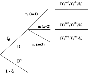
Figure 2. Illustration of information contained in the observations

where

$$\eta_{z}(i)=\begin{cases}1,&\text{if $A_{o}=z$ for the i-th subject},\\ 0,&\text{Otherwise}.\end{cases}\vspace{3mm}$$

The full likelihood, for the general case $z=1,2,...,l$ is,

(8) $$L_{a}=\Bigg{[}\prod_{i=1}^{s}(1-P)^{1-\xi_{i}}P^{\xi_{i}}\Bigg{]}\ \Bigg{[}\prod_{i=1}^{s}\Big{\{}\Big{(}\frac{dF(y_{i}^{bwd}+y_{i}^{fwd})}{\mu}\Big{)}^{\delta_{i}}\Big{(}\int_{\omega\geq y_{i}^{bwd}+c_{i}}\frac{dF(\omega)}{\mu}\Big{)}^{1-\delta_{i}}\prod_{z=1}^{l}P(A_{o}=z)^{\eta_{z}(i)}\Big{\}}^{\xi_{i}}\Bigg{]}.\vspace{5mm}$$

Using equation (7),

(9) $$\hat{\lambda}_{z}=\frac{\hat{P}(D_{\tau^{*}},A_{o}=z)}{\hat{\mu}_{z}P(A=z)}~{},$$

is the MLE of $\lambda_{z}$, where $\hat{\mu}_{z}$ is the MLE of $\mu_{z}$ derived from $\hat{S}_{z}$.

6. Estimating the incidence rate of dementia

In 1991, 10,263 elderly Canadians (65 years or older), living at home or in an institution, were screened for dementia (CSHA working group 1994). This phase of the study was known as CSHA-1. At the time of CSHA-1, 821 subjects were classified as having either possible Alzheimer’s disease, probable Alzheimer’s disease, or vascular dementia. Henceforth, by the term dementia we mean having exactly one of these three conditions since they constitute the vast majority of dementias. The approximate dates of onset were derived in a hierarchical fashion from the answers to three questions (Wolfson et al. 2001). In 1996, the second phase of the study, CSHA-2, was completed. CSHA-2 included the ascertainment of the date of death or right censoring for those cases identified at CSHA-1. These are the data upon which we shall base our estimates of the overall and age-specific incident rates of dementia. However, additional data were, in fact, collected as part of the CSHA with the goal of estimating the age-specific incidence rates of dementia among elderly Canadians. The subjects who were deemed not to have dementia at CSHA-1 were re-evaluated for dementia at CSHA-2. Assuming that these incidence rates had remained constant, they were estimated using the incident cases observed between CSHA-1 and CSHA-2. There were nevertheless, difficulties with these “incident” data since it could not be ascertained with certainty whether those who had died between CSHA-1 and CSHA-2 had become incident cases with dementia. In this paper we, therefore, re-estimated the incidence rates without relying on the “incident” cases that occurred between CSHA-1 and CSHA-2. The assumption of a roughly constant incidence rate for dementia has been previously checked in several ways and has been deemed to be reasonable (see Asgharian et al. 2002, Asgharian et al. 2006 and Addona and Wolfson 2006).

6.1. Estimating the overall incidence rate of dementia

The NPMLE, $\hat{S}(x)$, yields $\hat{\mu}\approx$ 4.75 years or 57 months. Since the CSHA data did not constitute a random sample of all subjects over the age of 65 in Canada, we used the age-standardized prevalence estimate instead of simply, $\hat{P}=\frac{N}{s}$ . This gives an estimate for $P$ of 0.066 (CSHA working group 1994), which leads to a point estimate, $\hat{\lambda}=$ 0.0139, or 13.9 per 1,000 person-years. To obtain an interval estimate for $\lambda$, we followed the bootstrap procedure and sampled with replacement from the 10,263 screened subjects to obtain 10,000 bootstrap samples of the same size. We obtained a confidence interval for $\lambda$ of $[12.52,15.28]$ cases per 1,000 person-years.

6.2. Estimating the age-specific incidence rate of dementia

Three age groups were considered for the CSHA data: 65-74, 75-84, and 85+ years old. The 821 cases of dementia were subdivided as follows: 164 had onset between 65 and 74 years old, 381 had onset between 75 and 84 years old, and 276 were 85 or older when they had onset. The estimated mean survival times in years were 7.97, 5.16, and 3.50, for the 65-74, 75-84, and 85+ groups, respectively. To use equation (9), we require an approximately stable age distribution over the period covering the onset times. We consulted data from four Canadian censuses covering 1976-1991 to assess this assumption. Figure 3 shows the progression of the percentage of the Canadian population aged 65 and older in each of the three age groups (Statistics Canada 2006). Using data from the 1976, 1981, 1986, and 1991 censuses, we also computed some measures of variability for the percentage in each of the three age groups. These are presented in Table 1.

Figure 3. Percentage of Canadian population aged 65 and older in 65-74 (circles), 75-84 (diamonds), and 85+ (triangles) age groups

Age Group	Range	SD	CV
65-74	59.8 - 62.7%	1.36%	0.022
75-84	29.1 - 31.3%	1.03%	0.034
85+	8.2 - 8.9%	0.34%	0.040

Table 1. Range, standard deviation, and coefficient of variation for the percentage of Canadians (aged 65 and older) in each age group

Having verified that the age distribution is roughly stable for this time period, we proceeded with the age-specific incidence estimation using the 1991 census data. Amongst those 65 years or older in 1991, 59.8% were in the 65-74 group, 31.3% were in the 75-84 group, and 8.9% were in the 85+ group (Statistics Canada 2006). The resulting age-specific incidence rate estimates are presented in Table 2. In 1976, amongst those 65 years or older, 62.7% were in the 65-74 group, 29.1% were in the 75-84 group, and 8.2% were in the 85+ group (Statistics Canada 2006). We also estimated the age-specific incidence rates based on the census age distribution data from 1976 to take into account small changes in the population age distribution that might have occurred over the period from 1976 to 1991. When the age distribution changes, this approach provides a simple framework for investigating robustness of the age-specific incidence rate estimator to departures from the assumption of constancy of the age distribution. For comparative purposes, the age-specific incidence rate estimates based on the 1976 census data are also given in Table 2.

Age Group	$\hat{\lambda}_{z}$ (1991)	95% CI (1991)	$\hat{\lambda}_{z}$ (1976)	95% CI (1976)
65-74	3.35	[2.72 , 3.99]	3.20	[2.58 , 3.82]
75-84	22.99	[19.92 , 26.04]	24.69	[21.26 , 28.13]
85+	85.86	[70.52 , 101.20]	93.39	[77.00 , 109.77]

Table 2. Age-specific incidence rate estimates per 1,000 person-years using 1991 and 1976 Canadian census data

6.3. Discussion of dementia incidence rate estimates

Subjects were not prospectively monitored between CSHA-1 and CSHA-2. It was thus difficult to ascertain whether those who had died in this time period had had onset of Alzheimer’s disease (possible or probable). As a result, incidence rates of Alzheimer’s disease reported from the CSHA were underestimates of the true incidence rates amongst elderly Canadians since they were based only on subjects who survived until the end of CSHA-2 in 1996. The CSHA incidence rate estimates of Alzheimer’s disease were 7.4 and 5.9 per 1,000 person-years for women and men respectively (CSHA working group 2000), giving a crude estimated incidence rate for men and women combined of 6.7 per 1000 person years. Using the CSHA data, Hébert et al.(2000) estimated the incidence rate of vascular dementia to be 3.79 per 1,000 person-years. Therefore the CSHA overall (under-) estimated rate for dementia was approximately 6.7 + 3.79 = 10.49 per 1000 person years. Direct comparison with our results is difficult. Our overall estimate (for possible or probable Alzheimer’s, or vascular dementia) of 13.9 per 1,000 person-years seems to be consistent with these previous estimates obtained from the CSHA. An analogous comparison of the age-specific incidence estimates reveals that they too are consistent with those already obtained from the CSHA. Note that the slightly different point estimates for the age-specific incidence rates, particularly in the 85+ category, should not be interpreted as meaning that incidence rates declined or increased between 1976 and 1991. They simply provide a range of possible values for the estimate depending on what is taken as the population age distribution.

7. Concluding remarks

Simulations, whose results are not reported in this paper, suggest that our methods work well for moderate sample sizes; the asymptotic distribution of the estimated incidence rates were close to Normal, the point estimates were close to their true values and the confidence intervals reasonably narrow for a range of parameter choices.

Our estimator of the incidence rate depends on the estimator $\hat{S}$, for the survival function $S$. We propose that the most efficient estimator for $S$, under the assumption of a constant incidence rate, should be used. The estimator, $\hat{S}$, used in this paper is more efficient than the well-known estimator of $S$ for general left truncation data (Wang 1991) which does not invoke stationarity of the incidence process (Asgharian et al. 2002). Indeed, it is possible to show that the estimators we present for the incidence rates (overall and age-specific) are asymptotically most efficient. This follows from Asgharian and Wolfson (2005, Theorem 3) and Van der Vaart (1998, Theorem 25.47, page 387).

If the largest observed failure time is censored, $\hat{S}$ is left undefined beyond this point by most authors. Consequently $\hat{\mu}$ is not well-defined in this situation. Fortunately, in our example, the largest survival time is a true failure time. Ad hoc “fixes” are available, but produce biased estimators.

The CSHA data used for illustration is based on an initial cohort of 10,263 subjects obtained as a stratified cluster sample whereby a fixed number of institutionalized (about 10%) and non-institutionalized (about 90%) subjects were sampled. In addition, those over 85 years old were over-sampled. We do not take into account the sampling scheme in our estimated incidence rates or in the asymptotic distributions of our estimators. To do so requires development of new theory allowing for within cluster dependence, which is a topic for further study and is not directly pertinent to our methods.

Appendix

We provide a road map of the proof of Theorem 1 and give further details about steps (iv) and (v) below. Road map of the proof:
(i) Establish the asymptotic behavior of $\hat{F}_{LB}$.
(ii) Establish the asymptotic behavior of $\hat{F}$ using (i).
(iii) Establish the asymptotic behavior of $\hat{\mu}$ using (ii).
(iv) Establish the independence of $\hat{\mu}$ and $\hat{P}$.
(v) Establish the asymptotic behavior of $\hat{\lambda}$ using (4), (iii), and (iv).
The derivation of (i) is similar to its counterpart given by Asgharian and Wolfson (2005), and those of (ii) and (iii) are similar to their counterparts in Asgharian et al. (2002). The expressions, however, are slightly different in view of the different sampling scheme under consideration here. We therefore sketch the proof of steps (iv) and (v).

Step(iv):
In this step we justify the independence of $\hat{P}$ and $\hat{F}$, and hence of $\hat{P}$ and $\hat{\mu}$. This independence is suggested by the likelihood factorization (3). Theorem 2 shows that this is in fact the case. First, observe that it follows from (2) that $\hat{P}=\frac{N}{s}$ is the NPMLE of $P$. We have

(10) $$\Pi_{s}=\sqrt{s}(\hat{P}-P)\stackrel{{\scriptstyle\mathscr{D}}}{{\to}}N\Big{(}0,P(1-P)\Big{)}\quad.$$

Theorem 2.

Let $\mathbb{R}\times D_{0}[0,t]$ be endowed with the topology induced by

$$\parallel(a,x)\parallel=\mid a\mid+\mathrm{sup}_{s\in[0,t]}\mid x(s)\mid\ \quad.$$

Under the assumptions of Theorem 1

$$(\Pi_{s},U_{N})\stackrel{{\scriptstyle\mathscr{D}}}{{\to}}(W,U)\qquad in\quad\mathbb{R}\times D_{0}[0,t]\ ,$$

where $U$ is given in Theorem 1 and $W\sim N(0,P(1-P))$ is independent of $U$.

Proof.

It follows from Theorem 7.2.1 and Lemma 7.2.1 of Cs$\ddot{o}$rgo and Revesz (1981) that

$$\parallel(\Pi_{s},U_{N})-(\Pi_{s},U_{[sP]})\parallel\stackrel{{\scriptstyle P}}{{\longrightarrow}}0\quad\text{as}\quad s\to\infty\$$

It remains to show that $\Pi_{s}$ and $U_{[sP]}$ are independent. This follows from the fact that $\hat{P}$ is a partial ancillary for $F_{LB}$, while $\{(Y_{i}^{bwd},Y_{i}^{obs},\delta_{i}),\quad i=1,2,\cdots,[sP]\}$ is partially sufficient for $F_{LB}$. ∎

Step(v):
In this final step we combine the results of steps (i) through (iii), in Theorem 1, to yield the asymptotic behaviour of $\hat{\lambda}$.

Proof of Theorem 1. Part (a) follows from Lemma 1, part (b) of Theorem 1 of Asgharian et al. (2002), and the asymptotic properties of the sample proportion in Binomial sampling. Part (b) follows from part (c) of Theorem 1 of Asgharian et al. (2002), (10), and the identity (4).                                                                                           $\Box$

References

1. Addona, V. and Wolfson, D. B. (2006). A formal test for the stationarity of the incidence rate using data from a prevalent cohort study with follow-up. Lifetime Data Analysis 12, No. 3, 267-284.
2. Alioum A., Commenges D., Thiébaut R., and Dabis F. (2005). A multistate approach for estimating the incidence of human immunodeficiency virus by using data from a prevalent cohort study. Applied Statistics 54, Part 4, 739-752.
3. Asgharian, M., M’Lan, C.E. and Wolfson, D. B. (2002). Length-biased sampling with right censoring: an unconditional approach. Journal of the American Statistical Association 97, No.457, 201-209.
4. Asgharian, M., and Wolfson, D.B. (2005). Asymptotic behaviour of the unconditional NPMLE of the length-biased survivor function from right censored prevalent cohort data. The Annals of Statistics 33, No.5, 2109-2131.
5. Asgharian, M., Wolfson, D. W. and Zhang, X. (2006). Checking stationarity of the incidence rate using prevalent cohort survival data. Statistics in Medicine 25, 1751-1767.
6. Biering-Sorensen, F., and Hilden, J. (1984). Reproducibility of the history of low-back trouble. Spine 9, No.3, 280-286.
7. Cox, D.R. (1969). Some sampling problems in technology. In New Developments in Survey Sampling. Edited by Johnson and Smith. Wiley, 506-527.
8. Csorgo, M. and Revesz (1981). Strong Approximation in Probability and Statistics. Academic Press, New York.
9. CSHA working group, (1994). Canadian study of health and aging: study methods and prevalence of dementia. Journal of the Canadian Medical Association 150, 899-913.
10. CSHA working group (2000). The incidence of dementia in Canada. Neurology 55, 66-73.
11. Diamond, I.D., and McDonald, J.W. (1991). Analysis of current-status data. In Demographic Applications of Event History Analysis Edited by Trussell, J., Hankinson, R., and Tilton, J. chapter 12. Oxford: Oxford University Press.
12. Folnegovic, Z. and Folnegovic-Smalc, V. (1992). Schizophrenia in Croatia: interregional differences in prevalence and a comment on constant incidence. Journal of Epidemiology and Community Health 46, 248-255.
13. Hébert, R., Lindsay, J., Verreault, R., Rockwood, K., Hill, G., and Dubois, M-F.(2000). Vascular dementia: Incidence and risk factors in the Canadian Study of Health and Aging. Stroke 31, 1487-1493.
14. Jemal, A., Murray, T., Ward, E., Samuels, A., Tiwari, R.C., Ghafoor, A., Feuer, E.J., and Thun, M.J. (2005). Cancer Statistics, 2005. CA: A Cancer Journal for Clinicians 55, 10-30.
15. Keiding, N. (2006). Event history analysis and the cross-section. Statistics in Medicine 25, 2343-2364.
16. Keiding, N. (1991). Age-specific incidence and prevalence: A statistical perspective (with discussion). Journal of the Royal Statistical Society, Series A 154, No.3, 371-412.
17. Keiding, N., Holst, C. and Green, A. (1989). Retrospective estimation of diabetes incidence from information in a current prevalent population and historical mortality. American Journal of Epidemiology 130, 588-600.
18. Neyman, J. (1955). Statistics-servant of all sciences. Science, Vol.122, no. 3166, 401-406.
19. Ogata, Y., Katsura, K., Keiding, N., Holst, C. and Green, A. (2000). Empirical Bayes age-period-cohort analysis of retrospective incidence data. Scandinavian Journal of Statistics 27, 415-432.
20. Patil, G.P. and Rao, C.R. (1978). Weighted distributions and sized-biased sampling with applications to wildlife populations and human families. Biometrics 34, 179-189.
21. Sorenson, E.J., Stalker, A.P., Kurland, L.T., and Windebank, A.J. (2002). Amyotrophic lateral sclerosis in Olmsted County, Minnesota, 1925 to 1998. Neurology 59, 280-282.
22. Statistics Canada (2006) Census of Population, Statistics Canada catalogue no. 97- 551-XCB2006005: Age Groups and Sex for the Population of Canada, Provinces and Territories, 1921 to 2006 Censuses. Ottawa: Statistics Canada.
23. Van der Vaart, A. W.(1998). Asymptotic Statistics. Cambridge Series in Statistics and Probabilistic Mathematics. Cambridge University Press, Cambridge, UK.
24. Vardi, Y. (1982). Nonparametric estimation in the presence of length bias. The Annals of Statistics 10, 616-620.
25. Vardi, Y. (1985). Empirical distributions in selection bias models. The Annals of Statistics 13, 178-205.
26. Vardi, Y. (1989). Multiplicative censoring, renewal processes, deconvolution and decreasing density: nonparametric estimation. Biometrika 76, No.4, 751-761.
27. Wang, M-C. (1991). Nonparametric estimation from cross-sectional survival data. Journal of the American Statistical Association 86, No.413, 130-143.
28. Wicksell, S.D. (1925). The Corpuscle Problem: A Mathematical Study of a Biometric Problem. Biometrika 17, No.1, 84-99.
29. Wolfson, C., Wolfson, D.B., Asgharian, M., M’Lan, C.E., Østbye, T., Rockwood, K. and Hogan, D.B.(2001). A reevaluation of the duration of survival after the onset of dementia. New England Journal of Medicine 344, No.15, 1111-1116.