Comment on “Failure of the Work-Hamiltonian Connection for Free-Energy Calculations”

J. Horowitz and C. Jarzynski

University of Maryland, College Park 20742

Nonequilibrium work relations establish a connection between nonequilibrium work values and equilibrium free energies. In a recent Letter, Vilar and Rubi [1] (VR) argue that the definition of work used in these relations,

$$W=\int dt\,\frac{\partial H}{\partial t}=\int dt\,\dot{\lambda}\,\frac{\partial H}{\partial\lambda},$$ (1)

is incorrect, and therefore the relations themselves are fundamentally flawed. In our investigations, however, we have reached the opposite conclusion [2], as have Imparato and Peliti [3] in direct response to VR.

In Eq. 1, $\lambda$ represents generalized coordinates ($a_{1},a_{2},\cdots$) describing the external bodies that we manipulate to act on the system of interest; $W$ is the integral of force, multiplied by the displacements of these bodies [4]. Referring to Refs. [2, 3, 4] for a broader discussion, in this Comment we illustrate that $W$ has exactly the properties we associate with thermodynamic work.

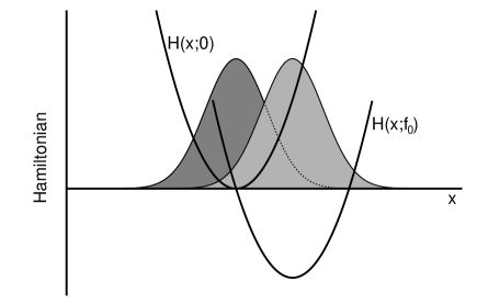
Figure 1: The Hamiltonian functions and equilibrium distributions (shaded) at $f=0$ and $f=f_{0}$.

We consider the model system analyzed in Ref. [1], described by the Hamiltonian

$$H(x;f)=\frac{1}{2}kx^{2}-fx,$$ (2)

and evolving under Langevin dynamics with friction coefficient $\gamma=1$. The force $f(t)$ is switched on uniformly, from $f(0)=0$ to $f(\tau)=f_{0}$; outside the time interval $0<t<\tau$ the force is held constant. This system evolves from equilibrium state $A$ in the distant past ($f=0$), to equilibrium state $B$ in the distant future ($f=f_{0}$). The initial and final Hamiltonian functions and canonical distributions are shown in Fig. 1. Since $H(x;f(t))$ is constant for $t<0$ and $t>\tau$, its value during these times is identified with the energy of the system [1]. Using the equilibrium distribution $p\propto\exp(-\beta H)$, we compute the internal energy ($E=\int pH$) and the entropy ($S=-\int p\ln p$) for states $A$ and $B$: $E_{A}=(2\beta)^{-1}$, $E_{B}=(2\beta)^{-1}-f_{0}^{2}/(2k)$, $S_{A}=S_{B}=[1-\ln(\beta k/2\pi)]/2$. From the thermodynamic definition of free energy, $G=E-ST$ [5], we then get

$$\Delta G=G_{B}-G_{A}=-\frac{f_{0}^{2}}{2k}.$$ (3)

The negative value of $\Delta G$ reflects a decrease in internal energy, with no change in entropy (see Fig. 1).

For this model, the distribution of work values over an ensemble of realizations of the process, $\rho(W)$, can be obtained using the approach of Ref. [6]. This distribution is a Gaussian with mean and variance,

$$\langle W\rangle=-\frac{f_{0}^{2}}{2k}+\frac{\beta\sigma_{W}^{2}}{2}\quad,\quad\sigma_{W}^{2}=\frac{2f_{0}^{2}}{\beta k^{2}\tau}\left[1+\frac{e^{-k\tau}-1}{k\tau}\right].$$ (4)

This result implies that: $W\rightarrow\Delta G$ for every realization in the reversible limit ($\tau\rightarrow\infty$); $\langle W\rangle>\Delta G$ in the irreversible case (finite $\tau$); and $\langle e^{-\beta W}\rangle=e^{-\beta\Delta G}$ for any value of $\tau$. Thus the work defined by Eq. 1 is consistent with the second law of thermodynamics, and its exponential average correctly gives $\Delta G$, when the free energy is defined by the expression $G=E-ST$.

By contrast, VR obtain $\Delta G>0$ for this model (Eq. 4 of Ref. [1]), and assert that a negative value would be “inconsistent with a nonspontaneous process”. We disagree. An undisturbed system certainly seeks to minimize its free energy (e.g., after the removal of a constraint), but when an external agent varies a parameter of the system, such as the field $f$ above, then there is no universal restriction on the sign of the free energy change. For instance, by manipulating a piston we can either increase or decrease the Helmholtz free energy of a gas, according to whether we compress or expand the gas.

References

- [1] J.M.G. Vilar and J.M. Rubi, Phys. Rev. Lett. 100, 020601 (2008).
- [2] C. Jarzynski, C. R. Physique 8, 495 (2007); J. Horowitz and C. Jarzynski, J. Stat. Mech. P11002 (2007).
- [3] A. Imparato and L. Peliti, arXiv:0707.3802v1; L. Peliti, J. Stat. Mech. P05002 (2008).
- [4] See e.g. J.W. Gibbs, Elementary Principles in Statistical Mechanics. Scribner’s, New York, 1902. Pages 42-44; K. Sekimoto, Prog. Theor. Phys. Suppl. 130, 17 (1998).
- [5] The distinction between Gibbs and Helmoltz free energies is not relevant for this model.
- [6] O. Mazonka and C. Jarzynski, arXiv:cond-mat/9912121 (1999).