Oscillations of the large-scale circulation in turbulent Rayleigh-Bénard convection: the off-center mode and its relationship with the torsional mode

Abstract

We report an experimental study of the large-scale circulation (LSC) in a turbulent Rayleigh-Bénard convection cell with aspect ratio unity. The temperature-extremum-extraction (TEE) method for obtaining the dynamic information of the LSC is presented. With this method, the azimuthal angular positions of the hot ascending and cold descending flows along the sidewall are identified from the measured instantaneous azimuthal temperature profile. The motion of the LSC is then decomposed into two different modes based on these two angles: the azimuthal mode and the translational or off-center mode that is perpendicular to the vertical circulation plane of the LSC. Comparing to the previous sinusoidal-fitting (SF) method, it is found that both the TEE and the SF methods give the same information about the azimuthal motion of the LSC, but the TEE method in addition can provide information about the off-center motion of the LSC. The off-center motion is found to oscillate time-periodically around the cell’s central vertical axis with an amplitude being nearly independent of the turbulent intensity. It is further found that the azimuthal angular positions of the hot ascending flow near the bottom plate and the cold descending flow near the top plate oscillate periodically out of phase by $\pi$, leading to the torsional mode of the LSC. These oscillations are then propagated vertically along the sidewall by the hot ascending and cold descending fluids. When they reach the mid-height plane, the azimuthal positions of the hottest and coldest fluids again oscillate out of phase by $\pi$. It is this out-of-phase horizontal positional oscillation of the hottest and coldest fluids at the same horizontal plane that produces the off-center oscillation of the LSC. A direct velocity measurement further confirms the existence of the bulk off-center mode of the flow field near cell center.

The paper has been submitted to J. Fluid Mech.

I Introduction

The convection phenomenon is ubiquitous in nature and in many engineering applications. A simple but paradigmatic model that has been widely used to study the convection phenomenon for more than a century is the turbulent Rayleigh-Bénard (RB) convection, which is a fluid layer heated from below and cooled on the top (for recent reviews, see siggia1994arfm ; agl2008rmp ). The dynamics of the RB system is determined by its geometry and two dimensionless control parameters: The Rayleigh number $Ra=\beta gH^{3}\Delta T/\nu\kappa$ and the Prandtl number $Pr=\nu/\kappa$, where $g$ is the gravitational acceleration, $H$ the height of the cell, $\Delta T$ the temperature difference across the cell, and $\beta$, $\nu$, and $\kappa$, respectively, the thermal expansion coefficient, the kinematic viscosity, and the thermal diffusivity of the fluid. The geometry of the system is described by its symmetry and the aspect ratio of the convection cell $\Gamma$. For a cylindrical cell, $\Gamma=D/H$ with $D$ being the cell’s diameter.

A prominent feature of turbulent RB system is the presence of the large-scale circulation (LSC), which is self-organized from thermal plumes that erupt from the top and bottom thermal boundary layers xi2004jfm . We call it “large-scale” because it is a single cellular structure that spans the height of the cell, at least in cells with aspect ratios close to one. In an axial symmetric configuration, the LSC is found to exhibit stochastic azimuthal meandering and small-probability events of cessations and reversals (see agl2008rmp and references therein). In addition, the horizontal motions of the LSC near the top and bottom plates are found to oscillate periodically out of phase by $\pi$. This twisting oscillation of the LSC’s vertical circulation plane is referred to as the torsional mode of the LSC, which was first found by Funfschilling $\&$ Ahlers funfschilling2004prl .

In addition to the torsional oscillation of the LSC, there also exists a well-defined low-frequency oscillation in both the temperature and velocity fields, which has been long observed in turbulent RB experiments using various fluids (see, e.g., castaing1989jfm ; takeshita1996prl ; ashkenazi1999prl ; qiu2001prl ; qiu2002pre ; lam2002pre ). As oscillation is a common phenomenon in closed flow systems, understanding the nature and the origin of the low-frequency oscillation in the RB system should be of general interest. To understand this oscillation, Villermaux villermaux1995prl proposed the coupled boundary layer model and the two main predictions of the model are: (1) Plumes are emitted periodically and (2) hot and cold plumes are emitted alternatively. The two predictions are not independent of each other. Physically speaking, thermal plumes can emit periodically but not necessarily alternatively. However, they cannot emit both alternatively and nonperiodically. This is because the alternative emission of hot and cold plumes implies a triggering mechanism of plume generation, i.e., hot plumes cause the emission of cold ones and vice versa. Therefore, the emission of one type of plumes should wait for the arrival of the other type. Since there exists a typical timescale for thermal plumes to travel from one plate to the other, the alternative emission process should quickly lead to a synchronized and periodic emission of hot and cold plumes from the bottom and top plates respectively. Some experiments based on single-point or two-dimensional (2D) measurements of the temperature and velocity fields appear to support Villermaux’s model ciliberto1996pre ; qiu2001prl ; qiu2002pre ; sun2005pre ; tsuji2005prl . Some other works, however, pointed out that periodic plume emission is not necessary for the periodicity of the system funfschilling2004prl ; resagk2006pof . Recently, Ahlers et al. agl2008rmp conjectured that the low-frequency oscillation of the system presumably is due to the torsional oscillation of the LSC. However, how the torsional mode generates the temperature and velocity oscillations at the mid-height plane of the cell is unclear, since, without the off-center oscillation, a simple twisting oscillation near the top and bottom plates would cancel out at the mid-height plane due to symmetry.

In a recent experimental study of the three-dimensional (3D) structure of temperature oscillations, Xi et al. xi2008prl have presented convincing evidences that hot and cold thermal plumes are emitted neither periodically nor alternatively, but continuously and randomly, from the top and bottom plates. Thus invalidate the two predictions of the Villermux’s model. They further showed that the low-frequency oscillation at the cell’s mid-height plane is due to the off-center oscillation of the LSC. It should be mentioned that a previous single-point velocity measurement has shown that at the cell center the strongest velocity oscillation is along the direction perpendicular to the LSC plane and that the strength of this oscillation decays away from the cell center towards the plates qiu2004pof . More recently, a study of the 3D spatial structure of the velocity field has shown that the velocities along the axis perpendicular to the LSC plane and at the cell’s mid-height plane correlate strongly with each other and have a common phase across the cell’s entire diameter sun2005pre . Both these results imply the existence of the off-center motion. However, the nature of this motion and its relationship with the torsional oscillation of the LSC have not been revealed, which are among the objectives of this paper.

The rest of the paper is organized as follows. We describe the experimental setup and conditions in Section 2.1. In Section 2.2, we describe in detail a method for extracting the azimuthal angular positions of the hottest and coldest fluids along the sidewall and the LSC’s central line from the measured instantaneous azimuthal temperature profile and provide a validation of this method. Comparisons with the previous sinusoidal-fitting method will also be made. The experiment results are presented and analyzed in Section 3, which is divided into three parts. In Section 3.1 we present a detailed study of the off-center oscillation of the LSC. Section 3.2 discusses the relationship between the off-center mode and the torsional mode of the LSC and Section 3.3 presents results from a direct velocity measurement of the bulk off-center mode of the flow field. We summarize our findings and conclude in Section 4.

II Experimental setup, methods and parameters

II.1 The convection cell and experiment conditions

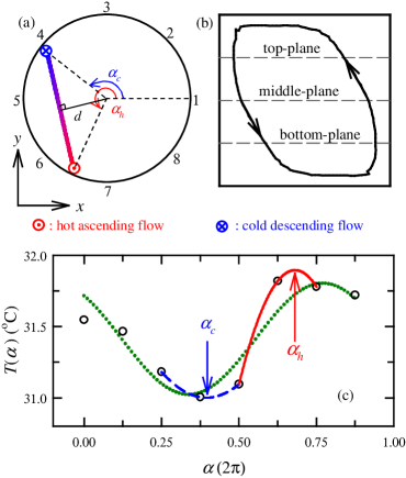
Figure 1: (a) Top-view of the convection cell and coordinate system used. Also shown is an actual instantaneous azimuthal positions $\alpha_{h}$ and $\alpha_{c}$ of the hot ascending and cold descending flows, corresponding to the temperature profile $T(\alpha)$ shown in (c). The $z$-axis (not shown in the figure) is along the cell’s central vertical axis. The numbers $1,2,\ldots,8$ show the locations of the sidewall thermistors. (b) Side-view of the cell with measured circulation path of the LSC reproduced from Ref. sunxia2005pre . The three dashed lines show the top, middle and bottom planes where the thermistors are placed. (c) An example of an actual instantaneous temperature profile (circles) measured by the 8 thermistors at mid-height plane at $Ra=5.5\times 10^{9}$. The solid line represents a quadratic fit to the highest temperature reading and the two temperature readings adjacent to it. The dashed line represents a quadratic fit to the lowest temperature reading and the two temperature readings adjacent to it. The two vertical arrows indicate the fitted peak positions of $\alpha_{h}$ and $\alpha_{c}$, respectively. The dotted line shows a sinusoidal fit to the profile. It is seen from the figure that, in this case, the sinusoidal fit to the profile shifts $\alpha_{h}$ to the right (anticlockwise in (a)) and shifts $\alpha_{c}$ to the left (clockwise in (a)).

The experiment was carried out in a cylindrical cell with its top and bottom plates made of 1.5-cm-thick copper, the sidewall of a 5-mm-thick Plexiglas tube and water as convection fluid xi2008pof . The inner diameter $D$ and the height $H$ of the cell are both 19.0 cm and hence its aspect ratio $\Gamma$ is unity. Twenty-four thermistors (Omega, 44031) with a diameter of 2.5 mm and an accuracy of $0.01^{\circ}$ were placed in blind holes drilled horizontally from the outside into the sidewall with a distance of 0.7 mm from the fluid-contact surface. These thermistors are distributed in three horizontal rows at distances $H/4$, $H/2$, and $3H/4$ from the bottom plate, which are denoted as the bottom, middle and top planes (the three dashed lines in figure 1(b)), respectively, and in eight vertical columns equally spaced azimuthally around the cylinder (figure 1(a)). A multichannel multimeter was used to record the resistances of the 24 thermistors at a sampling rate of 0.29 Hz, which are converted into temperatures using calibration curves. Then the azimuthal temperature profile $T(\alpha)$ at the three heights can be obtained, where $\alpha$ is the azimuthal angle referenced to location 1. During the measurements, the mean temperature $T_{0}$ of the bulk fluid was kept at $31^{\circ}$C and hence $Pr=5.3$. The measurements covered six values of $Ra$, ranging from $9.0\times 10^{8}$ to $6.0\times 10^{9}$, and lasted 70 to 750 hours.

In Ref. xi2008prl the cell was tilted by $2^{\circ}$ to study the origin of the temperature oscillations. This is because in addition to the twisting and off-center sloshing motion, the orientation of the LSC also meanders randomly. By tilting the cell and thus locking the LSC orientation, one can remove the stochastic meandering from the signal and separate the complicated phenomena produced by the different types of motions. This enabled us to study the phase relationships between temperature oscillations at various locations. In this work, our focus is on the relationship between the twisting motion near the top and bottom plates and the off-center motion at the mid-height plane. As the LSC meanders azimuthally as a whole across the height of the cell sun2005prl , the phase relationship between these two types of motions can be studied even with the azimuthal meandering present. Therefore, unless stated otherwise, all measurements in the present work were made with the cell levelled (to within $0\pm 0.06^{\circ}$).

As stated above, the temperature measurements in the present case are made with thermistors embedded in the sidewall, whereas in Ref. xi2008prl the off-center motion was obtained from thermistors placed in fluid. It is known that the sidewall acts as a low-pass filter, thus the thermistors embedded in the sidewall are not sensitive to the high-frequency signals. Spatially, they actually sense the integrated signal over a finite area of the sidewall, which leads to a lowered strength of the off-center oscillation as compared from that using the in-fluid probes. Nevertheless, as we will see below, the basic pictures obtained from the two cases are essentially the same. As one of the objectives of the present work is to understand the relationship between the off-center oscillation and the twisting oscillations near the plates, we use data measured simultaneously by the 24 in-wall probes from the three heights (there are only 8 in-fluid probes and that measurements can only be made at one height at a time). Thus, unless stated otherwise, all results presented in this paper were obtained from the in-wall probes.

II.2 The temperature-extremum-extraction method

An often-used method based on the multi-probe technique for extracting the dynamic information about the LSC motion is to fit the temperature azimuthal profile using a sinusoidal function, i.e. $T_{k}=T_{a}+A^{\prime}cos(k\pi/4-\phi^{\prime}),k=0,1,...,7$, where $T_{a}$ is the azimuthal average of the 8 temperature readings, $A^{\prime}$ is a measure of the strength of the LSC and $\phi^{\prime}$ is the LSC’s orientation (see, e.g. cioni1997jfm ; brown2005prl ; brown2006jfm ; xi2007pre ; xi2008pof ; funfschilling2008jfm ). This sinusoidal-fitting (SF) method has been very successful in the study of the azimuthal motion of the LSC, including rotations, cessations and reversals (see agl2008rmp and references therein). However, the SF method requires the separation between the hottest and coldest azimuthal positions to be $\pi$, i.e., the obtained LSC’s central line is forced to always pass through the cell’s central vertical axis, which, as we shall show below, is not always the case.

Here, we introduce the temperature-extremum-extraction (TEE) method that determines first the hottest and coldest azimuthal positions of the bulk fluid and then the central line of the LSC band. The TEE method has been described very briefly in Ref. xi2008prl . In this section, we give its detailed description, validation and comparison with the SF method. To illustrate this mehtod, figure 1(c) shows an example of the actual instantaneous temperature readings (circles) from the 8 thermistors at mid-height plane. The hottest (coldest) azimuthal position of the bulk fluid along the sidewall was determined by making a quadratic fit around the highest (lowest) temperature reading. In practice, this requires only the local maximum (minimum) temperature and the two temperatures directly adjacent to it. This is because a quadratic function has 3 degrees of freedom and thus can be uniquely determined by only 3 data points. We label these azimuthal positions $\alpha_{1}$, $\alpha_{2}$ and $\alpha_{3}$ with $\alpha_{2}$ being the position of the local maximum (minimum) temperature. The position $\alpha_{h}$ ($\alpha_{c}$) at any plane can then be found by solving analytically the 3 quadratic equations between $T({\alpha_{k}})$ and $\alpha_{k}$ ($k=1,2,3$), i.e.,

$$\alpha_{h}(\alpha_{c})=\frac{1}{2}\frac{(\alpha_{1}^{2}-\alpha_{2}^{2})[T(\alpha_{2})-T(\alpha_{3})]-(\alpha_{2}^{2}-\alpha_{3}^{2})[T(\alpha_{1})-T(\alpha_{2})]}{(\alpha_{1}-\alpha_{2})[T(\alpha_{2})-T(\alpha_{3})]-(\alpha_{2}-\alpha_{3})[T(\alpha_{1})-T(\alpha_{2})]}.$$ (1)

In this paper, the subscripts ‘$h$’ and ‘$c$’ are used to denote those quantities associated with the hot ascending and cold descending flows, respectively, and the subscripts ‘$t$’, ‘$m$’ and ‘$b$’ for the top, middle and bottom planes, respectively. To test the validity of the quadratic fit, figure 2 shows the normalized sidewall-temperature-profile. Each point is an average of $[T(\alpha_{k})-T_{0}]/\Delta T$ ($k=\alpha_{1},\alpha_{2},\alpha_{3}$) in a bin with a small range around $\alpha-\alpha_{h,m}$ (figure 2(a)) or $\alpha-\alpha_{c,m}$ (figure 2(b)). The data around the hottest (figure 2(a)) and coldest (figure 2(b)) positions are both in good agreement with the quadratic functions (solid lines), indicating that the quadratic function is indeed a good representation for the temperature distribution around the hot ascending and cold descending flows. With this method, the three rows of thermistors can thus provide simultaneously the azimuthal positions of the hot ascending and cold descending flows at the three heights, which are denoted as $\alpha_{h,t}$, $\alpha_{h,m}$, and $\alpha_{h,b}$, and $\alpha_{c,t}$, $\alpha_{c,m}$, and $\alpha_{c,b}$. With the obtained hottest and coldest positions, the line connecting the two positions is the central line of the LSC band. The orientation of this line is the orientation of the LSC, the distance between this line and the cell’s central vertical axis is defined as the off-center distance (see figure 1(a)) and $A=(T(\alpha_{h})-T(\alpha_{c}))/2$ is used to characterize the strength of the LSC, where the factor 1/2 is used in order to compare the obtained $A$ with that obtained from the SF method. We denote $\phi_{t}$, $\phi_{m}$, and $\phi_{b}$, $A_{t}$, $A_{m}$, and $A_{b}$, and $d_{t}$, $d_{m}$, and $d_{b}$ as the orientations, the strengths and the off-center distances of the LSC at the top, middle, and bottom planes, respectively. Therefore, based on the TEE method, the motion of the LSC can be decomposed into two different modes: The azimuthal mode and the off-center mode.

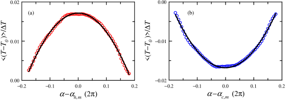
Figure 2: The averaged sidewall-temperature-profile $[T(\alpha)-T_{0}]$ normalized by the temperature difference $\Delta T$ around the fitted (a) hottest and (b) coldest azimuthal positions obtained at $Ra=5.5\times 10^{9}$. Solid lines are quadratic functions.

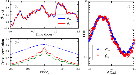
Figure 3: (a) Time traces of the orientation $\phi_{m}$ of the LSC central line obtained using the TEE method and the orientation $\phi^{\prime}_{m}$ obtained from the SF method. (b) The cross-correlation functions between the orientations obtained using the two different methods for the top (solid line), middle (dashed line) and bottom (dotted line) planes. (c) PDF of the two orientations $\phi_{m}$ and $\phi^{\prime}_{m}$. All data were measured at $Ra=5.5\times 10^{9}$.

We now compare the orientations and the strengths of the LSC obtained using the TEE method and those obtained using the SF method. Figure 3(a) shows the time traces of $\phi_{m}$ and $\phi^{\prime}_{m}$, which are obtained using the same data set measured by the embedded thermistors. One sees that the time traces are very similar to each other. This similarity can be characterized by the coefficient of the cross-correlation between the two quantities. The cross-correlation function between two variables $a$ and $b$ is defined as

$$C_{a,b}(\tau)=\langle(a(t+\tau)-\langle a\rangle)(b(t)-\langle b\rangle)\rangle/a_{rms}b_{rms},$$ (2)

where $a_{rms}$ and $b_{rms}$ are standard deviations of $a$ and $b$, respectively, and $\langle\cdots\rangle$ represents the temporal average. When $a=b$, $C_{a,a}$, denoted as $C_{a}$, is the auto-correlation function of the variable $a$. Figure 3(b) shows the cross-correlation functions between $\phi$ and $\phi^{\prime}$ at the three heights. It shows that all these three functions have a positive and strong correlation with the coefficient being all larger than 0.85 at time lag $\tau=0$. (The subpeaks of $C_{\phi_{t},\phi^{\prime}_{t}}$ and $C_{\phi_{b},\phi^{\prime}_{b}}$ correspond to the twisting oscillations of the LSC near the top and bottom plates.) It is further found that this strong positive correlation exists for all values of $Ra$ investigated. Figure 3(c) shows the probability density functions (PDF) of $\phi_{m}$ and $\phi^{\prime}_{m}$. One sees that the two PDFs essentially collapse on top of each other except that the distribution of $\phi^{\prime}_{m}$ seems to be a little smoother than that of $\phi_{m}$.

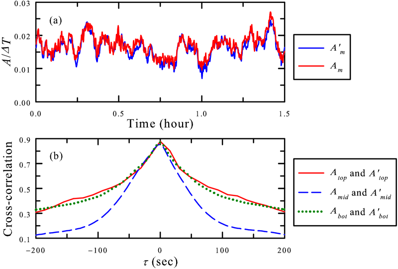
Figure 4: (a) Time traces of the normalized strength $A_{m}/\Delta T$ of the LSC obtained using the TEE method and the normalized strength $A^{\prime}_{m}/\Delta T$ obtained from the SF method. (b) The cross-correlation functions between the strengths obtained using the two different methods for the top (solid line), middle (dashed line) and bottom (dotted line) planes. The data were measured at $Ra=5.5\times 10^{9}$.

Figure 4(a) shows the time traces of $A_{m}$ and $A^{\prime}_{m}$. It is seen that the two time traces are again very similar to each other except that $A_{m}$ is on average $\sim 5\%$ larger than $A^{\prime}_{m}$. Figure 4(b) shows the cross-correlation functions between $A$ and $A^{\prime}$ at the three heights. It similarly shows that all three functions have a strong positive correlation with their peaks all located at time lag $\tau=0$ and the cross-correlation coefficient $C(\tau=0)$ all being nearly 0.9.

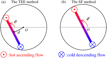
Figure 5: (a) Schematic diagram showing the definitions of the orientation $\phi$ and the off-center distance $d$ of the LSC obtained using the TEE method. (b) Schematic diagram showing the definition of the orientation $\phi^{\prime}$ of the LSC obtained using the SF method. In this method, the off-center distance is forced to be always zero.

The above results imply that, as far as the orientation and the strength of the LSC are concerned, both the SF and TEE methods give the same results, but the TEE method in addition determines the LSC’s off-center motion, which is missed by the SF method. This is illustrated in figures 5(a) and (b). It is also clear that the LSC’s orientation is determined mainly by the hottest and coldest azimuthal positions of the bulk fluid along the sidewall. This is not surprising, since one can see from figure 1(c) that the sinusoidal fit to the temperature profile shifts the hottest azimuthal position $\alpha_{h,m}$ right or anticlockwise and shifts the coldest azimuthal position $\alpha_{c,m}$ left or clockwise and the changes of the obtained orientation of the LSC due to the two shifts roughly cancel each other.

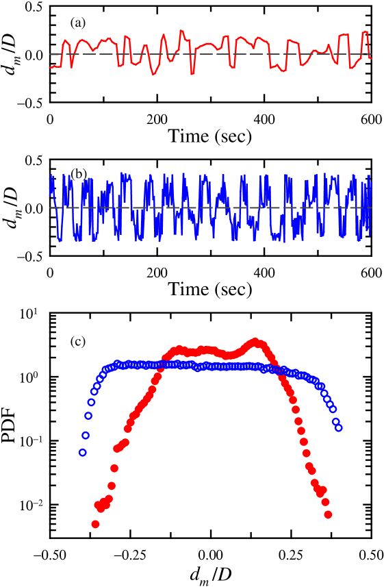
Figure 6: (a, b) Time traces of the normalized off-center distance $d_{m}/D$ from thermistors (a) embedded into the sidewall and (b) placed in fluid. (c) PDF of $d_{m}/D$ from the in-wall (solid circles) and in-fluid (open circles) thermistors. The data of the in-fluid thermistors are taken at $Ra=5.0\times 10^{9}$ with a sampling rate of 0.76 Hz and that of the in-wall probes at $Ra=5.5\times 10^{9}$ with a sampling rate of 0.29 Hz.

III Results and discussion

III.1 The off-center oscillation of the LSC at mid-height plane

The off-center distance $d_{m}$ of the LSC’s central line at the mid-height plane is used to study the off-center motion of the LSC at that plane. Figure 6(a) shows a typical time trace of the measured $d_{m}$ normalized by the cell’s diameter $D$. It is seen from the figure that $d_{m}/D$ fluctuates around 0. We further found that the temporal averages of $d_{m}/D$ for all six values of $Ra$ are nearly 0. In Ref. xi2008prl a similar trace measured with the in-fluid thermistors in a tilted cell has been shown. For comparison, we plot in figure 6(b) a time trace of $d_{m}/D$ measured under the same conditions as in Ref. xi2008prl but with the cell leveled ($0\pm 0.06^{\circ}$). It shows that $d_{m}/D$ measured from the in-fluid probes has a stronger strength and its oscillation looks more periodic when compared with that obtained from the in-wall thermistors. Nevertheless, the physical pictures revealed by the two time traces are the same, i.e., the LSC’s central line oscillates horizontally around the cell’s central vertical axis. Figure 6(c) shows the PDF of $d_{m}/D$ obtained from the in-wall thermistors (solid circles). The PDF is found to be flatter than a Gaussian function, i.e. the flatness is $2.3$. The PDFs obtained at other $Ra$ share the same features as that shown in figure 6(c), except for the two lowest $Ra$ which is probably due to the limited temperature contrast along the sidewall. For comparison, we also plot the PDF of $d_{m}/D$ obtained from the in-fluid thermistors (open circles). It is seen that the PDF from the in-fluid probes is even flatter (flatness 1.9) than that from the in-wall thermistors, reflecting a larger range of oscillation.

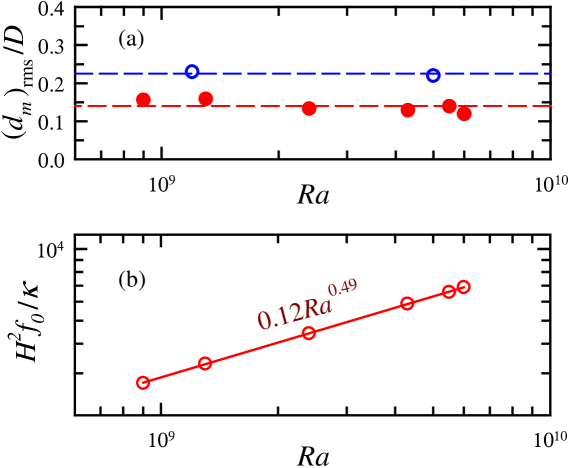
Figure 7: (a) The $Ra$-dependence of the standard deviation of $d_{m}/D$ from the in-wall (solid circles) and in-fluid (open circles) thermistors. Two dashed lines show the mean value of $d_{m}/D$ averaged over all $Ra$ investigated. (b) Normalized oscillation frequency $H^{2}f_{0}/\kappa$ obtained from the frequency power spectra of $d_{m}$ as a function of $Ra$. The solid line is the power-law fit.

As $d_{m}/D$ oscillates around its mean value of 0, its standard deviation $(d_{m})_{rms}/D$ can be used as a measure of the amplitude of this oscillation. Figure 7(a) shows the $Ra$-dependence of $(d_{m})_{rms}/D$ obtained from the in-wall (solid circles) and in-fluid (open circles) thermistors. One sees that $(d_{m})_{rms}/D$ depends weakly on $Ra$ for the present range of $Ra$ with $(d_{m})_{rms}/D$ from the in-fluid probes being $\sim 60\%$ larger than that obtained from the in-wall thermistors. In Ref. xi2008prl it has been shown that the off-center or sloshing motion of the LSC exhibits a well-defined time-periodic oscillation. The prominent peak near $f_{0}$ in the frequency power spectra of $d_{m}$ (see the second curve from bottom in figure 8(a)) corresponds to this periodic oscillation. In figure 7(b) we plot the $Ra$-dependence of the normalized frequency corresponding to this prominent peak obtained from the spectra of $d_{m}$. The solid line in the figure represents the power-law fit to the data: $H^{2}f_{0}/\kappa=0.12Ra^{0.49\pm 0.02}$, with the scaling exponent being in good agreement with the previous temperature measurements in water qiu2001prl ; qiu2002pre ; sunxia2005pre ; brown2007jstat , mercury takeshita1996prl and low-temperature helium gas heslot1987pra ; castaing1989jfm ; sano1989pra ; niemela2001jfm . This result further indicates that the previously-observed temperature oscillations near the mid-height of the cell indeed originates from the off-center oscillation of the LSC. Taken together, the physical picture behind figure 6 is that the LSC’s central line oscillates time-periodically around the cell’s central vertical axis with an amplitude nearly independent of the turbulent intensity.

III.2 The relationship between the off-center mode and the torsional mode of the LSC

Figure 8: From top to bottom: Power spectra of (a) $\phi_{t}$, $\phi_{m}$, $\phi_{b}$, $d_{t}$, $d_{m}$, and $d_{b}$, and (b) $\alpha_{h,t}$, $\alpha_{h,m}$, $\alpha_{h,b}$, $\alpha_{c,t}$, $\alpha_{c,m}$, and $\alpha_{c,b}$. All data have been shifted vertically for clarity.

Figure 8(a) shows, from top to bottom, the frequency power spectra of $\phi_{t}$, $\phi_{m}$, $\phi_{b}$, $d_{t}$, $d_{m}$, and $d_{b}$. For the orientations of the LSC obtained at the three heights, the prominent peak near $f_{0}$ representing periodic oscillation can be seen clearly for $\phi_{t}$ and $\phi_{b}$, but is absent for the mid-height plane ($\phi_{m}$). These are consistent with those observed by Ref. funfschilling2008jfm and correspond to the twisting mode of the LSC funfschilling2004prl . We further found that although $\phi_{m}$ will also exhibit oscillation when the cell is tilted by several degrees, the strength of this oscillation obtained at the mid-height plane is much weaker than those of $\phi_{t}$ and $\phi_{b}$, i.e., the peak height of the spectra of $\phi_{m}$ at $f_{0}$ is much smaller than those of $\phi_{t}$ and $\phi_{b}$. However, for the off-center distance, the situation is opposite. In figure 8(a) one sees that the strength of the oscillation peak for $d_{m}$ at the mid-height plane is much stronger than those of $d_{t}$ and $d_{b}$.

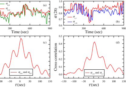
Figure 9: Time traces of (a) $\alpha_{h,b}$ and $\alpha_{h,m}$ and of (b) $\alpha_{c,t}$ and $\alpha_{c,m}$. The cross-correlation functions between (c) $\alpha_{h,m}$ and $\alpha_{h,b}$ and between (d) $\alpha_{c,m}$ and $\alpha_{c,t}$. All data were obtained at $Ra=5.5\times 10^{9}$.

To understand this difference and to find out the relationship between the off-center mode at the mid-height plane and the torsional mode of the LSC near the top and bottom plates, we examine the frequency power spectra of the azimuthal positions of the hot ascending and cold descending flows at the three heights, as both the orientation $\phi$ and the off-center distance $d$ of the LSC are obtained from these positions. Figure 8(b) shows that the spectra of $\alpha_{c,t}$ and $\alpha_{h,b}$ exhibit an oscillation peak near $f_{0}$. Whereas the spectra of $\alpha_{h,t}$ and $\alpha_{c,b}$ both give very faint oscillations, which is due to a tilted ellipselike circulation path of the LSC when viewed from the side (Qiu $\&$ Tong 2001b; Sun $\&$ Xia 2005; Sun et al. 2005b). The thermistors embedded into the sidewall can not feel accurately the hot ascending flow of the LSC at the top-plane and the cold descending flow of the LSC at the bottom-plane, since they are far away from the sidewall at the respective heights (figure 1(b)). Therefore, at the top and bottom planes, the in-wall probes may not be able to measure the orientation and the off-center distance of the LSC as accurately as those at the mid-height plane. This suggests that the relatively weak oscillation peaks of $d_{t}$ and $d_{b}$ shown in figure 8(a) are mainly due to the oscillations of $\alpha_{c,t}$ and $\alpha_{h,b}$. The surprising thing shown in figure 8(b) is that the spectra of the azimuthal positions $\alpha_{h,m}$ and $\alpha_{c,m}$ of the hot ascending and cold descending flows at the mid-height plane both exhibit a well-defined time-periodic oscillation with the oscillation peak located at $f_{0}$ and with the same strength as those of $\alpha_{h,b}$ and $\alpha_{c,t}$. This implies that the azimuthal positions of the hot ascending and cold descending fluids both oscillate periodically along the sidewall irrespective of whether they are near the plates or at the mid-height of the cell.

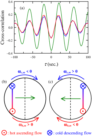
Figure 10: (a) The cross-correlation functions $C_{\omega_{c,t},\omega_{h,b}}$ (blue line) and $C_{\omega_{c,m},\omega_{h,m}}$ from the in-wall (red line) and in-fluid thermistors (dark green line). The data from in-wall thermistors are taken at $Ra=5.5\times 10^{9}$ and that from in-fluid probes at $Ra=5.0\times 10^{9}$. (b) Schematic diagram of the azimuthal positions of the hot ascending and cold descending flows when the off-center oscillation is at an extremum. The curved arrows show the directions of the angular velocities and the horizontal arrow shows the moving direction of the LSC’s central line. (c) Same as (b) but half an oscillation period later.

Figure 9(a) shows typical time traces of $\alpha_{h,b}$ and $\alpha_{h,m}$ measured at the same time. It is seen that the two time traces are rather similar to each other except for a several-second delay between them. The cross-correlation function $C_{\alpha_{h,m},\alpha_{h,b}}$ shown in figure 9(c) quantifies this similarity. It shows that $\alpha_{h,m}$ and $\alpha_{h,b}$ have a strong positive correlation with the main peak located at $\tau\simeq 6\pm 1$ s. This positive time-delay indicates that the azimuthal motion of $\alpha_{h,m}$ lags that of $\alpha_{h,b}$, which is easy to understand since the hot ascending flow rises up from bottom. Similar situation can be seen for the relation between $\alpha_{c,t}$ and $\alpha_{c,m}$. Figure 9(b) shows the time traces of $\alpha_{c,t}$ and $\alpha_{c,m}$, which again are quite similar to each other. Figure 9(d) plots $C_{\alpha_{c,m},\alpha_{c,t}}$, and it is found that $\alpha_{c,m}$ correlates strongly with $\alpha_{c,t}$ with a positive time delay $\tau\simeq 5\pm 1$ s indicating that the azimuthal motion of $\alpha_{c,m}$ lags that of $\alpha_{c,t}$. Here we note that the time delay of the main peak of $C_{\alpha_{c,m},\alpha_{c,t}}$ is essentially the same as that of $C_{\alpha_{h,m},\alpha_{h,b}}$ within experimental uncertainty, this is due to the fact that the distance between the middle and the top planes is the same as the distance between the middle and bottom ones. Note also that the subpeaks of $C_{\alpha_{h,m},\alpha_{h,b}}$ and $C_{\alpha_{c,m},\alpha_{c,t}}$ correspond to the periodic oscillations shown in figure 8(b). These results further imply that the hot ascending and cold descending flows go up and fall down coherently, thus propagate their azimuthal positional oscillations along the sidewall.

The torsional mode of the LSC can be revealed by the horizontal motions of the hot ascending and cold descending flows near the top and bottom plates. Here, we define

$$\omega_{i,j}=d\alpha_{i,j}/dt,$$ (3)

as the azimuthal angular velocity of $\alpha_{i,j}$, where $i=h$ or $c$ and $j=t$, $m$, or $b$. Figure 10(a) shows the cross-correlation function $C_{\omega_{c,t},\omega_{h,b}}$ between $\omega_{c,t}$ and $\omega_{h,b}$ (blue line). It is seen that $C_{\omega_{c,t},\omega_{h,b}}$ oscillates and $\omega_{c,t}$ anticorrelates with $\omega_{h,b}$ with a strong negative peak located at $\tau=0$. The negative peak at $\tau=0$ indicates that $\alpha_{c,t}$ rotates clockwise when $\alpha_{h,b}$ rotates anticlockwise and vice versa, implying the twisting motion of the LSC. Recall that the azimuthal motions of $\alpha_{h,m}$ and $\alpha_{c,m}$ follow coherently those of $\alpha_{h,b}$ and $\alpha_{c,t}$, respectively, with the same time delay. The azimuthal angular velocities of $\alpha_{h,m}$ and $\alpha_{c,m}$ would hence be expected to exhibit the same behavior as those of $\alpha_{h,b}$ and $\alpha_{c,t}$, and this is indeed observed from figure 10(a), which shows that $C_{\omega_{c,m},\omega_{h,m}}$ (red line) is the same as $C_{\omega_{c,t},\omega_{h,b}}$ (blue), i.e. periodic oscillations and a strong negative peak at $\tau=0$. Here, we also plot $C_{\omega_{c,m},\omega_{h,m}}$ obtained from the in-fluid thermistors (dark green line). It is seen that $C_{\omega_{c,m},\omega_{h,m}}$ obtained from the in-fluid thermistors exhibits the oscillation with much stronger periodicity than that obtained from the in-wall thermistors (red line). However, the basic picture is the same for both cases. These results indicate that the azimuthal positional oscillations of the hot ascending and cold descending flows at the mid-height plane are out of phase with each other by $\pi$, leading to the off-center mode of the LSC at the mid-height plane. The mechanism of how this off-center mode is generated is illustrated in figures 10(b) and (c). Figure 10(b) shows that $\alpha_{c,m}$ rotates clockwise when $\alpha_{h,m}$ rotates anticlockwise, and the line connecting them thus moves to the right. Half an oscillation period later (figure 10(c)), the motion of $\alpha_{c,m}$ changes to anticlockwise while that of $\alpha_{h,m}$ to clockwise. This makes the LSC central line move to the left. The periodic occurrence of this process thus generates the off-center oscillation of the LSC and produces the prominent peak near $f_{0}$ on the spectra of $d_{m}$. On the other hand, as the orientation $\phi_{m}$ equals to $(\alpha_{h,m}+\alpha_{c,m})/2$ plus a constant, the anticorrelation between $\omega_{h,m}$ and $\omega_{c,m}$ would cancel out the periodic oscillations, and hence it is not surprising to see in figure 8(a) that an oscillation peak is absent for the spectra of $\phi_{m}$.

III.3 Direct velocity measurement of the off-center motion

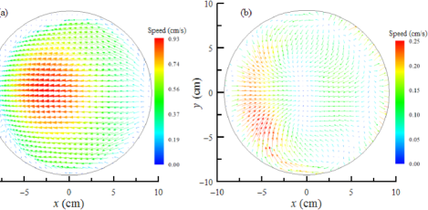
Figure 11: Time-averaged velocity vector map measured (a) near the top plate and (b) at the mid-height plane. For clarity, a coarse-grained vector map of size $32\times 32$ is shown. The magnitude of the velocity $\sqrt{u^{2}+v^{2}}$ is coded in both the color and the length of the arrows in units of cm/s. Both time-averages are taken over a period of 151 min corresponding to 20000 velocity maps.

We present in this subsection direct evidence of the off-center oscillation of the LSC from particle image velocimetry (PIV) measurement of the horizontal velocity field at the mid-height plane in a sapphire cell. Both the sapphire cell and the horizontal velocity measurement using the PIV technique have been described in detail previously xi2006pre ; zhou2007prl and hence we outline only their main features here. The sapphire cell consists of two sapphire discs with thickness 5 mm as the top and bottom plates and a Plexiglas tube with thickness 8 mm as the sidewall. The cell’s inner diameter and height are both 18.5 cm, so the aspect ratio of the cell is also unity. In the present work, 50-$\mu$m-diameter polyamid spheres (density 1.03 gcm^-3) were used as the seeding particles and a horizontal laser light-sheet with thickness $\sim 2$ mm was used to illuminate the particles in the mid-height plane of the cell. The measuring area is a square of $18.5\times 18.5$ cm², which covers completely the horizontal cross-section of the cell. The spatial resolution is 0.29 cm, corresponding to $63\times 63$ velocity vectors in each 2D velocity map. Denote the laser-illuminated plane as the $(x,y)$-plane and the center of the mid-height horizontal cross-section of the cell as the origin $O$ of the coordinates (see figure 13(a)), then two horizontal velocity components $u(x,y)$ and $v(x,y)$ are measured. In these PIV measurements, the cell was tilted by $\sim 1^{\circ}$ at position 1, and thus the orientation of the LSC was locked along the $x$-direction (see figure 1(a)). For the PIV experiment, the measurements were made at $Ra=3.0\times 10^{9}$ and $6.0\times 10^{9}$ and at $Pr=4.3$. A total of 20000 vector maps were acquired for each $Ra$ at a sampling rate of $\sim 2.2$ Hz. As the two measurements give the same results, only results for $Ra=6.0\times 10^{9}$ will be presented.

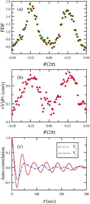
Figure 12: (a) PDF of the orientation $\theta$ of the spatially averaged vector $\vec{V}$. (b) The conditional average $\langle V|\theta\rangle$ on the velocity orientation $\theta$. (c) The auto-correlation functions of $V_{x}$ and $V_{y}$.

To study the global motion of the central bulk fluid, we use the velocity vector $\vec{V}(t)=V_{x}(t)\hat{x}+V_{y}(t)\hat{y}$ to characterize the overall flow behavior at the mid-height plane, where $V_{x}(t)$ and $V_{y}(t)$ are the spatial averages of the local velocity components $u(t)$ and $v(t)$, respectively, within a circular area centered at the center of the measurement area. The diameter of the circular area is 5 cm and there are 221 vectors contained in this circular region for averaging. A circle with a diameter of 10 cm has also been used and the obtained results are essentially the same xi2006pre . The orientation $\theta\equiv\arctan(V_{y}/V_{x})$ and the magnitude $V\equiv|\vec{V}|=\sqrt{V_{x}^{2}+V_{y}^{2}}$ of the averaged vector are then measures of the orientation and the strength of the motion of the central bulk fluid, respectively.

Note that the horizontal velocity field investigated in Ref. xi2006pre was obtained near the top plate. Figure 11(a) shows the time-averaged velocity vector map measured at 2 cm from the top plate, which shows that the LSC is dominated mainly by the horizontal velocities. Thus, the spatial averaged velocity vector $\vec{V}(t)$ measured at the horizontal planes near the top plate can be used as a measure of the orientation vector $\vec{V}_{LSC}$ of the LSC xi2006pre and its orientation $\theta$ can be used to characterize the orientation of the LSC at the corresponding height. However, the situation is different when the measurement is made near the cell’s mid-height plane. Figure 11(b) shows the time-averaged velocity vector map obtained at the mid-height horizontal plane of the cell. Because at the cell’s mid-height plane the LSC is concentrated near the sidewall and dominated mainly by vertical velocities (see the circulation path of the LCS shown in figure 1(b)), the velocity vector $\vec{V}(t)$ spatially averaged from the velocities in the central bulk region cannot be used to represent the orientation vector of the LSC and its orientation $\theta$ is no longer a direct measure of the LSC’s orientation. Therefore, $\theta$ and $\phi_{m}$ (the orientation of the LSC obtained from the azimuthal temperature profile) would exhibit different behaviors. As we shall see below, this is indeed the case.

Figure 12(a) shows the PDF of the measured velocity orientation $\theta$. It is seen that the PDF of $\theta$, which is significantly different from that of $\phi_{m}$ in figure 3(c), exhibits a bimodal distribution with two peaks located at the orientations ($\theta=\pm 0.25$) that are perpendicular to the preferred orientation of the LSC ($\theta=0$). The probabilities of $\theta=\pm 0.25$ are nearly 3 times larger than those of $\theta=0$ and $\theta=\pm 0.5$, suggesting that the central bulk fluid is much more likely to move in the direction perpendicular to the LSC’s vertical circulation plane rather than in the LSC’s preferred direction itself. To study the flow strength of the central bulk fluid in different orientations, we calculate the conditional average $\langle V|\theta\rangle$ on the velocity orientation $\theta$, as shown in figure 12(b). One sees that the averaged velocity magnitudes in the directions ($\theta=\pm 0.25$) perpendicular to the LSC plane are much stronger than the magnitudes in all other directions, especially than that in the preferred direction of the LSC. Figure 12(c) shows the auto-correlation functions $C_{V_{x}}$ (dashed line) and $C_{V_{y}}$ (solid line). Both show oscillations, but the oscillation strength of $V_{y}$ (in the direction perpendicular to the LSC plane) is much stronger than that of $V_{x}$ (along the LSC’s preferred direction) and $V_{y}$ oscillates more coherently than $V_{x}$. In fact, a previous single-point velocity measurement has shown that at the cell center the strongest velocity oscillation is along the direction perpendicular to the LSC plane and that the strength of this oscillation decays away from the cell center towards the plates qiu2004pof ; sun2005pre . We further note that the oscillation frequency of $V_{y}$ is the same as that of the off-center motion of the LSC but $20\%$ larger than that of $V_{x}$. The existence of two different oscillation frequencies in turbulent convection with fixed control parameters ($Ra$ and $Pr$) have already been observed previously xi2006pre ; brown2007jstat , but the reason(s) for the presence of two clocks in turbulent RB system remain unknown xia2007jstat . Here we offer a possible reason for the observed different oscillation frequencies of $V_{x}$ and $V_{y}$. Even though the convection cell has been tilted by $\sim 1^{\circ}$ in the PIV measurement, the orientation of the LSC can still meander around the locked direction (the $x$-axis in the present case) over an azimuthal angular range of a few tens degrees ahlers2006jfm . The projection of the off-center oscillation onto the $x$-direction would thus generate the oscillation in $V_{x}$, while the stochastic fluctuations of the projection angle would both reduce the coherence and change the frequency of the oscillation of $V_{x}$. Note that the different oscillation frequencies for $V_{x}$ and $V_{y}$ have also been observed, but not explicitly recognized, by Refs. qiu2004pof and sun2005pre . Notwithstanding the above, the overall picture emerging from the PIV measurements is that the translational motion of the central bulk fluid in the direction perpendicular to the LSC’s vertical circulation plane is more probable, much stronger and more coherent than the motions in all other directions, which provides a direct evidence for the off-center motion of the LSC at the mid-height plane.

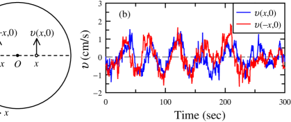
Figure 13: (a) Coordinate system and schematic diagram of the mid-height horizontal cross-section of the cell. The origin $O$ of the coordinates is chosen as the center of the cross-section and thus the $z$-axis (not shown in the figure) is along the cell’s central vertical axis. The two vertical arrows show the velocity components $v$ located at positions $(x,0)$ and $(-x,0)$ and the dashed line shows the $x$-axis. (b) Time traces of $v(x,0)$ and $v(-x,0)$ for $x/D=0.11$.

In a previous work, Sun et al. sun2005pre measured the 2D velocity field in the $(y,z)$-plane, which is perpendicular to the LSC’s vertical circulation plane and studied the phase relationships among the horizontal velocity components $v(y)$ along the $y$-axis and among $v(z)$ along the $z$-axis. For $v(y)$ along the $y$-axis, their results showed that the velocity component $v(y)$ at different values of $y$ are highly correlated and have a common phase across the cell’s entire diameter. For $v(z)$ along the $z$-axis, their results revealed that the horizontal velocity component $v(z)$ at different height $z$ remain in phase along the $z$-axis mainly in the middle one-half of the cell, while the horizontal velocity components $v(z)$ near the upper and lower conducting plates gradually lag behind those in the central region of the cell. Both of these results imply that the motion of the central bulk fluid is spatially coherent and the off-center oscillation is the dominant mode of the central bulk fluid motion.

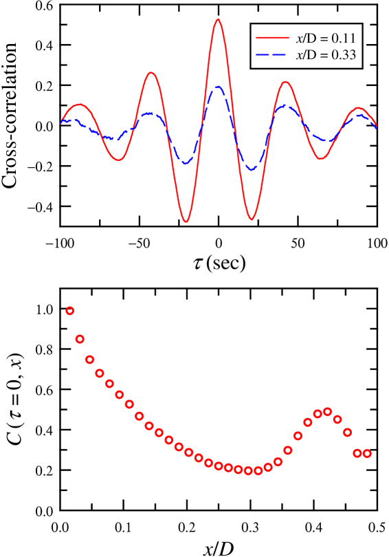
Figure 14: (a) The cross-correlation functions $C(\tau,x)$ between $v(x,0)$ and $v(-x,0)$ for $x/D=0.11$ (solid line) and $0.33$ (dashed line). (b) The cross-correlation coefficient $C(\tau=0,x)$ as a function of $x$.

The bulk off-center mode of the flow field can also be revealed by investigating the variation along the $x$-axis of the $y$ velocity component $v(x,0)$. Here we study the relationship between $v(x,0)$ and $v(-x,0)$ for various values of $x(>0)$. If the azimuthal rotation is the dominant motion of the LSC, $v(x,0)$ should anticorrelate with $v(-x,0)$, i.e., $v(x,0)$ is along the $y$-direction when $v(-x,0)$ is along the $-y$-direction and vice versa. While $v(x,0)$ correlates strongly with $v(-x,0)$ for the situation that the off-center motion is the LSC’s dominant mode, i.e., $v(x,0)$ and $v(-x,0)$ are along the same direction. Figure 13(b) shows the typical time series of $v(x,0)$ and $v(-x,0)$ for $x/D=0.11$. It is seen that $v(x,0)$ and $v(-x,0)$ are very similar to each other and along the same direction for most of the time. In addition, both $v(x,0)$ and $v(-x,0)$ are found to exhibit a well-defined periodic oscillation, corresponding to the off-center oscillation of the LSC. To characterize quantitatively these features, figure 14(a) shows the cross-correlation functions $C(\tau,x)$ between $v(x,0)$ and $v(-x,0)$ for $x/D=0.11$ (solid line) and 0.33 (dashed line). It shows that both functions oscillate and have a large positive peak located at $\tau=0$, indicating that $v(x,0)$ correlates strongly with $v(-x,0)$. It is further found that this peak exists for all $x$ and all horizontal velocity oscillations of $v(x,0)$ have a common phase across the cell’s entire diameter. Figure 14(b) shows the cross-correlation coefficient $C(\tau=0,x)$ as a function of $x$. One sees that $C(\tau=0,x)\gtrsim 0.2$ for all $x$ and it has a peak near the sidewall (around $x/D\simeq 0.42$). The peak of $C(\tau=0,x)$ near the sidewall represents the anticorrelation between $\omega_{h,m}$ and $\omega_{c,m}$, i.e. the off-center motion of the LSC, as illustrated in figures 10(b) and (c). Both the strong positive peak located at $\tau=0$ and the oscillation of the cross-correlation functions $C(\tau,x)$ between $v(x,0)$ and $v(x,0)$ for all $x$ reveal the fact that the dominant motion of the LSC at the mid-height plane is indeed the off-center oscillation, which provides another direct evidence for the off-center mode of the LSC at the mid-height plane.

IV Conclusion

To conclude, we have made a detailed experimental study of the oscillations of the large-scale circulation (LSC) in a cylindrical turbulent Rayleigh-Bénard convection cell with aspect ratio unity using water as working fluid. Direct spatial measurements of both the temperature and velocity fields were carried out to study the motion of the LSC.

Direct measurements of the horizontal velocity field at the cell’s mid-height plane using the PIV technique were made at $Ra=3.0\times 10^{9}$ and $6.0\times 10^{9}$ and $Pr=4.3$. It is found that the horizontal translational motion of the central bulk fluid in the direction perpendicular to the vertical circulation plane of the LSC is more probable, much stronger and more coherent than the motions in all other directions. For the velocity component $v(x,0)$ perpendicular to the LSC plane, $v(x,0)$ for all values of $x$ are found to correlate strongly with each other, especially for the velocities near the sidewall, and have a common phase across the cell’s entire diameter. Both of these results provide direct evidences for the off-center mode of the LSC at the mid-height plane.

The temperature measurement was performed over the Rayleigh-number range $9\times 10^{8}\leq Ra\leq 6\times 10^{9}$ and at fixed Prandtl number $Pr=5.3$. At each $Ra$ the instantaneous azimuthal temperature profile along the sidewall at three different heights, i.e. $H/4$, $H/2$, and $3H/4$ from the bottom plate, were measured. To study the motion of the LSC, we developed a new method, the temperature-extremum-extraction (TEE) method. Using this method, the azimuthal angular positions of the hot ascending and cold descending flows at each height were obtained by making a quadratic fit around the highest and lowest temperature readings, respectively, and the line connecting these two positions is the central line of the LSC band. The orientation of this line is thus the orientation of the LSC and the distance between this line and the cell’s central vertical axis is defined as the off-center distance. The motion of the LSC is therefore decomposed into two different modes: the azimuthal mode and the translational or off-center mode. When compared to the sinusoidal-fitting (SF) method, it is found that, as far as the azimuthal motion of the LSC is concerned, the two methods give the same information in terms of both the orientation and the flow strength of the LSC, while the TEE method can in addition determine the LSC’s off-center motion that is missed by the SF method. With the TEE method, the LSC’s central line is found to oscillate time-periodically around the cell’s central vertical axis with an amplitude being nearly independent of the turbulent intensity, leading to the off-center oscillation of the LSC.

Results obtained using the TEE method further reveal that both the torsional and off-center modes of the LSC are manifestations of the out-of-phase azimuthal positional oscillations of the hot ascending and cold descending flows. When these two flows are near the top and bottom plates, the resulting motion is torsional. When they are near the mid-height plane, the resulting motion is the off-center oscillation.

- (1) Ahlers, G., Brown, E. Nikolaenko, A. 2006 The search for slow transients, and the effect of imperfect vertical alignment, in turbulent Rayleigh-Bénard convection J. Fluid Mech. 557, 347-367.
- (2) Ahlers, G., Grossmann, S. Lohse, D. 2008 Heat transfer and large scale dynamics in turbulent Rayleigh-Bénard convection Rev. Mod. Phys. submitted.
- (3) Ashkenazi, S. Steinberg, V. 1999 High Rayleigh number turbulent convection in a gas near the gas-liquid critical point. Phys. Rev. Lett. 83, 3641-3644.
- (4) Brown, E. Ahlers, G. 2006 Rotations and cessations of the large-scale circulation in turbulent Rayleigh-Bénard convection. J. Fluid Mech. 568, 351-386.
- (5) Brown, E., Funfschilling, D. Ahlers, G. 2007 Anomalous Reynolds-number scaling in turbulent Rayleigh-Bénard convection. J. Statist. Mech., P10005.
- (6) Brown, E., Nikolaenko, A. Ahlers, G. 2005 Reorientation of the large-scale circulation in turbulent Rayleigh-Bénard convection. Phys. Rev. Lett. 95, 084503.
- (7) Castaing, B., Gunaratne, G., Heslot, F., Kadanoff, L., Libchaber, A., Thomae, S., Wu, X.-Z., Zaleski, S. Zanetti, G. 1989 Scaling of hard thermal turbulence in Rayleigh-Bénard convection. J. Fluid Mech. 204, 1-30.
- (8) Ciliberto, S., Cioni, S. Laroche, C. 1996 Large-scale flow properties of turbulent thermal convection. Phys. Rev. E 54, R5901-R5904.
- (9) Cioni, S., Ciliberto, S. Sommeria, J. 1997 Strongly turbulent Rayleign-Bénard convection in mercury: Comparison with results at moderate Prandtl number. J. Fluid Mech. 335, 111-140.
- (10) Funfschilling, D. Ahlers, G. 2004 Plume motion and large-scale circulation in a cylindrical Rayleigh-B enard cell. Phys. Rev. Lett. 92, 194502.
- (11) Funfschilling, D., Brown, E. Ahlers, G. 2008 Torsional oscillations of the large-scale circulation in turbulent Rayleigh-Bénard convection. J. Fluid Mech. 607, 119-139.
- (12) Heslot, F., Castaing, B. Libchaber, A. 1987 Transitions to turbulence in helium gas. Phys. Rev. A 36, 5870-5873.
- (13) Lam, S., Shang, X.-D., Zhou, S.-Q. Xia, K.-Q. 2002 Prandtl number dependence of the viscous boundary layer and the Reynolds numbers in Rayleigh-Bénard convection. Phys. Rev. E 65, 066306.
- (14) Niemela, J. J., Skrbek, L., Sreenivasan, K. R. Donnelly, R. J. 2001 The wind in confined thermal convection. J. Fluid Mech. 449, 169-178.
- (15) Qiu, X.-L. Tong, P. 2001a Onset of Coherent Oscillations in Turbulent Rayleigh-B nard Convection. Phys. Rev. Lett. 87, 094501.
- (16) Qiu, X.-L. Tong, P. 2001b Large-scale velocity structures in turbulent thermal convection. Phys. Rev. E 64, 036304.
- (17) Qiu, X.-L. Tong, P. 2002 Temperature oscillations in turbulent Rayleigh-Bénard convection. Phys. Rev. E 66, 026308.
- (18) Qiu, X.-L., Shang, X.-D., Tong, P. Xia, K.-Q. 2004 Velocity oscillations in turbulent Rayleigh-Bénard convection. Phys. Fluid 16, 412-423.
- (19) Resagk, C., du Puits, R., Thess, A., Dolzhansky, F., Grossmann, S., Fontenele Araujo, F. Lohse, D. 2006 Oscillations of the large scale wind in turbulent thermal convection. Phys. Fluids 18, 095105.
- (20) Sano, M., Wu, X.-Z. Libchaber, A. 1989 Turbulence in helium-gas free convection. Phys. Rev. A 40, 6421-6430.
- (21) Siggia, E. D. 1994 High Rayleigh number convection. Annu. Rev. Fluid. Mech. 26, 137-168.
- (22) Sun, C., Xi, H.-D. Xia, K.-Q. 2005a Azimuthal symmetry, flow dynamics, and heat flux in turbulent thermal convection in a cylinder with aspect ratio one-half. Phys. Rev. Lett. 95, 074502.
- (23) Sun, C. Xia, K.-Q. 2005 Scaling of the Reynolds number in turbulent thermal convection. Phys. Rev. E 72, 067302.
- (24) Sun, C., Xia, K.-Q. Tong, P. 2005b Three-dimensional flow structures and dynamics of turbulent thermal convection in a cylindrical cell. Phys. Rev. E 72, 026302.
- (25) Takeshita, T., Segawa, T., Glazier, J. A. Sano, M. 1996 Thermal turbulence in Mercury. Phys. Rev. E 76, 1465-1468.
- (26) Tsuji, Y., Mizuno, T., Mashiko, T. Sano, M. 2005 Mean Wind in Convective Turbulence of Mercury. Phys. Rev. Lett. 94, 034501.
- (27) Villermaux, E. 1995 Memory-induced low frequency oscillations in closed convection boxes. Phys. Rev. Lett. 75, 4618-4621.
- (28) Xi, H.-D., Lam, S. Xia, K.-Q. 2004 From laminar plumes to organized flows: the onset of large-scale circulation in turbulent thermal convection. J. Fluid Mech. 503, 47-56.
- (29) Xi, H.-D. Xia, K.-Q. 2007 Cessations and reversals of the large-scale circulation in turbulent thermal convection. Phys. Rev. E 75, 066307.
- (30) Xi, H.-D. Xia, K.-Q. 2008 Flow mode transitions in turbulent thermal convection. Phys. Fluids 20, 055104.
- (31) Xi, H.-D., Zhou, Q. Xia, K.-Q. 2006 Azimuthal motion of the mean wind in turbulent thermal convection. Phys. Rev. E 73, 056312.
- (32) Xi, H.-D., Zhou, S.-Q., Zhou, Q., Chan, T.-S. Xia, K.-Q. 2008 Origin of the temperature oscillation in turbulent thermal convection. Phys. Rev. Lett. submitted.
- (33) Xia, K.-Q. 2007 Two clocks for a single engine in turbulent convection. J. Statist. Mech. N11001.
- (34) Zhou, Q., Sun, C. Xia, K.-Q. 2007 Morphological evolution of thermal plumes in turbulent Rayleigh-Bénard convection. Phys. Rev. Lett. 98, 074501.