Hole spin relaxation in $p$-type GaAs quantum wires investigated by numerically solving fully microscopic kinetic spin Bloch equations

Abstract

We investigate the spin relaxation of $p$-type GaAs quantum wires by numerically solving the fully microscopic kinetic spin Bloch equations. We find that the quantum-wire size influences the spin relaxation time effectively by modulating the energy spectrum and the heavy-hole–light-hole mixing of wire states. The effects of quantum-wire size, temperature, hole density, and initial polarization are investigated in detail. We show that, depending on the situation, the spin relaxation time can either increase or decrease with hole density. Due to the different subband structure and effects arising from spin-orbit coupling, many spin-relaxation properties are quite different from those of holes in the bulk or in quantum wells, and the inter-subband scattering makes a marked contribution to the spin relaxation.

I Introduction

Spintronics is continuing to attract considerable interest because of its potential application to information technology.spintronics Several spintronics devices have been proposed that manipulate spin via spin-orbit coupling (SOC).datta ; Loss ; filter In recent years, progress in nanofabrication and growth techniques has made it possible to produce high-quality quantum wires (QWRs) and investigate spin physics in semiconductor nanostructures.Quay ; Ritchie ; Hirayama The energy spectrum of QWR systems with strong SOC has been extensively studied.Cahay2 ; Liu ; Ulrich1 ; Ulrich2 ; Hausler ; Arakawa ; Bastard ; Kapon ; Fasolino ; Chang ; Bimberg ; Vlaev It is well known that, even in the absence of an external magnetic field, the RashbaRashba and DresselhausDresselhaus SOCs lift the spin degeneracy in wire subbands at nonzero wave vectors. The subband structure for quantum-confined valence-band states is particularly interesting since they are subject to an especially strong SOC.Ulrich1 ; Ulrich2 ; Arakawa ; Bastard ; Chang ; Kapon ; Fasolino ; Sherman ; Bimberg ; Vlaev

As a long spin relaxation time (SRT) is desirable for the operation of spintronic devices, many investigations have been performed to better understand the electron spin relaxation in quantum structures,Bleibaum ; Cahay1 ; Ridley ; Raimondi ; Ando ; Rossler ; Flatte ; Bottesi ; Privman ; Yoh ; Smith ; Balents ; Wu1 ; Wu2 ; Wu3 ; Weng ; Wu5 ; review ; Cheng ; schu ; Zhou ; Zhou2 ; Cheng2 ; Clv e.g., using the single-particle modelRossler ; Flatte ; Bleibaum ; Cahay1 ; Ridley ; Raimondi ; Ando or Monte-Carlo simulations.Privman ; Yoh ; Cahay1 However, it was shown by Wu et al.Wu1 ; Wu2 ; Wu3 ; Weng ; Wu5 that the single-particle approach is inadequate in accounting for the spin relaxation. A fully microscopic kinetic spin Bloch equation (KSBE) theory, which takes full account of the inhomogeneous broadening from the Dresselhaus and/or Rashba SOC and the effect of scattering, has been developed to study spin relaxation.review ; Wu1 ; Wu2 ; Wu3 ; Weng ; Wu5 Cheng et al. applied this approach (excluding the Coulomb scattering) to study electron spin relaxation in QWR systems and showed the feasibility of manipulating spin decoherence.Cheng Investigations of spin relaxation of holes in QWRs are relatively limited,Ando even though knowledge of hole spin relaxation in $p$-type QWRs is important for assessing the feasibility of hole-based spintronic devices.ohno The spin-relaxation mechanism in hole QWRs can be expected to be quite different from that in electron systems, and 2D or bulk hole systems, due to the strong SOC and the complex wire-subband structure. These effects have not been addressed previously.

In this paper, we investigate hole spin relaxation in a $p$-doped (001) GaAs QWR. An idealized system of quantum wire with rectangular confinements and hard wall potential is considered in our calculation. First, we obtain the subband structure by diagonalizing the hole Hamiltonian including the quantum confinement. Here the light-hole (LH) admixture is dominant in the lowest spin-split subband, but the heavy-hole (HH) admixture becomes also important in higher subbands due to the strong HH-LH mixing. Then we investigate the time evolution of holes by numerically solving the fully microscopic KSBEs in the obtained subbands, with all the scattering, particularly the Coulomb scattering, explicitly included. We find that the QWR size influences the SRT effectively because the SOC and the subband structure in QWRs depend strongly on the confinement. When the QWR size increases, the lowest spin-split subband and the second-lowest spin-split subband will get very close to each other at an anticrossing point. If the anticrossing is close to the Fermi surface, the contribution from spin-flip scattering reaches a maximum and, correspondingly the SRT will reach a minimum. Moreover, we show that the dependence of the SRT on confinement size in QWRs behaves oppositely to the trend found in quantum wells. It is also found that, when the QWR size is very small, the SRT can either increase or decrease with hole density, depending on the spin mixing of the subbands. However, the behavior of holes in QWRs where the SRT increases or decreases with hole density is quite different from the one of LHs in quantum wells with small well width.Clv These features originate from the subband structure of the QWRs and the spin mixing which give rise to the spin-flip scattering. The spin mixing and inter-subband scattering are modulated more dramatically in QWRs by changing the hole distribution in different subbands. We also investigate the effects of temperature and initial spin polarization, showing that the inter-subband scattering and the Coulomb Hartree-Fock contribution can make a marked contribution to the spin relaxation.

This paper is organized as follows: In Sec. II we set up our model and the KSBEs. Our numerical results are presented in Sec. III. We conclude in Sec. IV.

II Model and KSBE

Our investigation considers a rectangular $p$-doped (001) GaAs QWR confined in both $x$ and $y$ directions as shown schematically in Fig. 1. The potential height of the barrier layer is assumed to be infinite, and the QWR size in the $x$ ($y$) direction is $a_{x}$ ($a_{y}$). Here the $x$, $y$ and $z$ directions correspond to the [100], [010] and [001] crystallographic directions, respectively. We assume that the conduction and valence bands are decoupled, and the effect of the split-off band is neglected because the spin-orbit split-off energy in bulk GaAs is much larger than the energy gap between the subbands caused by the confinement considered here. Then, based on the four-band Luttinger-Kohn model, lutt the explicit matrix form of the 4$\times$4 bulk-hole Hamiltonian in the basis of spin-3/2 projection ($J_{z}$) eigenstates with quantum numbers $+\frac{3}{2}$, $+\frac{1}{2}$, $-\frac{1}{2}$ and $-\frac{3}{2}$ can be written asWinkler_book

$$H_{h}=\left(\begin{array}[]{cccc}H_{hh}&S&R&0\\ S^{\dagger}&H_{lh}&0&R\\ R^{\dagger}&0&H_{lh}&-S\\ 0&R^{\dagger}&-S^{\dagger}&H_{hh}\end{array}\right)+H_{8v8v}^{r}+H_{8v8v}^{b}+V_{c}({\bf r}),$$ (1)

where $V_{c}({\bf r})$ is the hard-wall confinement potential in $x$ and $y$ directions and

$$H_{hh}=\frac{1}{2m_{0}}[(\gamma_{1}+\gamma_{2})[P_{x}^{2}+P_{y}^{2}]+(\gamma_{1}-2\gamma_{2})P_{z}^{2},$$ (2)

$$H_{lh}=\frac{1}{2m_{0}}[(\gamma_{1}-\gamma_{2})[P_{x}^{2}+P_{y}^{2}]+(\gamma_{1}+2\gamma_{2})P_{z}^{2},$$ (3)

$$S=-\frac{\sqrt{3}\gamma_{3}}{m_{0}}P_{z}[P_{x}-iP_{y}],$$ (4)

$$R=-\frac{\sqrt{3}}{2m_{0}}\{\gamma_{2}[P_{x}^{2}-P_{y}^{2}]-2i\gamma_{3}P_{x}P_{y}\},$$ (5)

$$H_{8v8v}^{r}=\frac{\gamma^{8v8v}_{41}}{\hbar}[J_{x}(P_{y}{\cal E}_{z}-P_{z}{\cal E}_{y})+J_{y}(P_{z}{\cal E}_{x}-P_{x}{\cal E}_{z})$$

$$\ \ \ \ \ \ \ \ +J_{z}(P_{x}{\cal E}_{y}-P_{y}{\cal E}_{x})],$$ (6)

$$H_{8v8v}^{b}=\frac{b^{8v8v}_{41}}{\hbar^{3}}\{J_{x}[P_{x}(P_{y}^{2}-P_{z}^{2})]+J_{y}[P_{y}(P_{z}^{2}-P_{x}^{2})]$$

$$\ \ \ \ \ \ \ \ +J_{z}[P_{z}(P_{x}^{2}-P_{y}^{2})]\}.$$ (7)

In these equations, $m_{0}$ denotes the free electron mass, $\gamma_{1}$, $\gamma_{2}$ and $\gamma_{3}$ are the Luttinger parameters, ${\cal E}$ is the electric field, and $J_{i}$ are spin-3/2 angular momentum matrices.lutt $H_{8v8v}^{r}$ is the SOC arising from the structure inversion asymmetry (SIA) and $H_{8v8v}^{b}$ is the SOC from the bulk inversion asymmetry (BIA). These two terms turn out to be one or two orders of magnitude smaller than the intrinsic SOC from the four-band Luttinger-Kohn Hamiltonian [the first term in Eq. (1)]. This can be seen from Appendix A where we present a comparison between spin splittings due to the SIA and BIA and the splitting from the intrinsic SOC. Moreover, from the first term in Eq. (1), one can see that the LH spin-up states can be directly mixed with the HH states by $S$ and $R$, but the mixing between LH spin-up states and LH spin-down states has to be mediated by the HH states. All the mixing is related to the confinement. When the confinement decreases, the mixing increases due to the decrease of the energy gap between the LH and HH states.

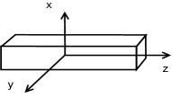
Figure 1: Schematic geometry of the QWR.

We construct the KSBEs by using the nonequilibrium Green function method as follows:review

$$\dot{\bf{\rho}}_{{k}}+\dot{\bf{\rho}}_{{k}}|_{coh}+\dot{\bf{\rho}}_{{k}}|_{scatt}=0.$$ (8)

Here ${\bf{\rho}}_{{k}}$ represents a single-particle density matrix of holes with wave vector $k$ along the $z$-axis. One can project $\rho_{{k}}$ in the collinear spin space which is constructed by basis $\{s\}$, with $\{s\}$ obtained from the eigenfunctions of the diagonal part of $H_{h}(k)$. $|s\rangle=|m,n\rangle|\sigma\rangle$ with $\langle r|m,n\rangle=\frac{2}{\sqrt{a_{x}a_{y}}}\sin(\frac{m\pi y}{a_{y}})\sin(\frac{n\pi x}{a_{x}})e^{i{k}z}$ and $|\sigma\rangle$ standing for the eigenstates of $J_{z}$. Then the matrix elements in the collinear spin space $\rho^{c}_{k,s_{1},s_{2}}$ is written as $\rho^{c}_{k,s_{1},s_{2}}=\langle s_{1}|\rho_{k}|s_{2}\rangle$. Here the superscript “$c$” denotes the quantum number distinguishing states in the collinear spin space. One can also project $\rho_{k}$ in the “helix” spin space which is constructed by basis $\{\eta\}$ with $\eta$ being the eigenfunctions of $H_{h}(k)$:

$$H_{h}(k)|\eta\rangle=E_{\eta,k}|\eta\rangle.$$ (9)

This basis function is a mixture of LH and HH states and is $k$ dependent. Then the matrix elements in the helix spin space $\rho^{h}_{{k},\eta,\eta^{\prime}}$ can be written as $\rho^{h}_{{k},\eta,\eta^{\prime}}=\langle\eta|\rho_{k}|\eta^{\prime}\rangle$, with the superscript “$h$” denoting the helix spin space. The density matrix in the helix spin space can be transformed from that in the collinear one by a unitary transformation: $\rho^{h}_{k}=U^{\dagger}_{k}\rho_{k}^{c}U_{k}$, where $U_{k}(i,\alpha)=\eta^{i}_{\alpha}(k)$ with $\eta^{i}_{\alpha}(k)$ being the $i$th element of the $\alpha$th eigenvector after the diagonalization of $H_{h}(k)$.

In this paper we project the density matrix in the helix spin spaceCheng2 and then the coherent terms can be written as

$$\dot{\rho}^{h}_{{k}}|_{coh} = -i\Big{[}\sum_{\bf Q}V_{\bf Q}U^{\dagger}_{k}I_{\bf Q}U_{k-q}{\rho}^{h}_{k-q}U^{\dagger}_{k-q}I_{\bf-Q}U_{k},\rho^{h}_{k}\Big{]}$$ (10)

$$\mbox{}-i\Big{[}U^{\dagger}_{k}H_{h}(k)U_{k},\rho^{h}_{k}\Big{]},$$

where $[A,B]=AB-BA$ denotes the commutator, and $I_{\bf Q}$ is the form factor in the collinear spin space with wave vector ${\bf Q}\equiv(q_{x},q_{y},q)$. The first term in Eq. (10) is the Coulomb Hartree-Fock term, and the second term is the contribution from the intrinsic SOC from the Luttinger-Kohn Hamiltonian. $I_{\bf Q}$ can be written as $I_{{\bf Q},s_{1},s_{2}}=\langle s_{1}|e^{i{\bf Q}\cdot{\bf r}}|s_{2}\rangle=\delta_{\sigma_{1},\sigma_{2}}F(m_{1},m_{2},q_{y},a_{y})F(n_{1},n_{2},q_{x},a_{x})$, with

$$F(m_{1},m_{2},q,a)=2iaq[e^{iaq}\cos{\pi(m_{1}-m_{2})}-1]\left[\frac{1}{\pi^{2}(m_{1}-m_{2})^{2}-a^{2}q^{2}}-\frac{1}{\pi^{2}(m_{1}+m_{2})^{2}-a^{2}q^{2}}\right].$$ (11)

For small spin polarization, the contribution from the Hartree-Fock term in the coherent term is negligibleWeng ; schu and the spin precession is determined by the SOC, $\dot{\rho}^{h}_{{k},\eta,\eta^{\prime}}|_{coh}=-i\rho^{h}_{{k},\eta,\eta^{\prime}}(E_{\eta,k}-E_{\eta^{\prime},k})$, which is proportional to the energy gap between $\eta$ and $\eta^{\prime}$ subbands.

The scattering terms include the hole-nonmagnetic-impurity, hole-phonon and hole-hole Coulomb scatterings. In the helix spin space, The scattering terms are given by

$$\dot{\rho}^{h}_{{k}}|_{scat} = \pi N_{i}\sum_{{\bf Q},\eta_{1},\eta_{2}}|U^{i}_{\bf Q}|^{2}\delta(E_{\eta_{1},k-q}-E_{\eta_{2},k})U^{\dagger}_{k}I_{\bf Q}U_{k-q}[(1-{\rho}^{h}_{k-q})T_{k-q,\eta_{1}}U^{\dagger}_{k-q}I_{-{\bf Q}}U_{k}T_{k,\eta_{2}}{\rho}^{h}_{k}$$ (12)

$$\mbox{}-\rho^{h}_{k-q}T_{k-q,\eta_{1}}U^{\dagger}_{{k-q}}I_{-{\bf Q}}U_{k}T_{k,\eta_{2}}(1-\rho^{h}_{k})]+\pi\sum_{{\bf Q},\eta_{1},\eta_{2},\lambda}|M_{{\bf Q},\lambda}|^{2}U^{\dagger}_{k}I_{\bf Q}U_{k-q}\{\delta(E_{\eta_{1},k-q}-E_{\eta_{2},k}+\omega_{{\bf Q},\lambda})$$

$$\mbox{}\times[(N_{{\bf Q},\lambda}+1)(1-{\rho}^{h}_{k-q})T_{k-{q},\eta_{1}}U^{\dagger}_{k-q}I_{-{\bf Q}}U_{k}T_{{k},\eta_{2}}{\rho}^{h}_{k}-N_{{\bf Q},\lambda}\rho^{h}_{k-q}T_{{k}-q,\eta_{1}}U^{\dagger}_{{\bf k-q}}I_{-{\bf Q}}U_{k}T_{k,\eta_{2}}(1-\rho^{h}_{k})]$$

$$\mbox{}+\delta(E_{\eta_{1},k-q}-E_{\eta_{2},k}-\omega_{{\bf Q},\lambda})[N_{{\bf Q},\lambda}(1-{\rho}^{h}_{k-q})T_{{k}-q,\eta_{1}}U^{\dagger}_{k-q}I_{-{\bf Q}}U_{{k}}T_{k,\eta_{2}}{\rho}^{h}_{k}$$

$$-(N_{{\bf Q},\lambda}+1)\rho^{h}_{k-q}T_{{k}-q,\eta_{1}}U^{\dagger}_{k-q}I_{-{\bf Q}}U_{k}T_{k,\eta_{2}}(1-\rho^{h}_{k})]\}$$

$$\mbox{}+\pi\sum_{{\bf Q},k^{\prime}}\sum_{\eta_{1},\eta_{2},\eta_{3},\eta_{4}}V_{\bf Q}^{2}U^{\dagger}_{k}I_{\bf Q}U_{k-q}\delta(E_{\eta_{1},{k}-q}-E_{\eta_{2},k}+E_{\eta_{3},k^{\prime}}-E_{\eta_{4},k^{\prime}-q})$$

$$\mbox{}\times\{(1-{\rho}^{h}_{k-q})T_{k-q,\eta_{1}}U^{\dagger}_{k-q}I_{-{\bf Q}}U_{k}T_{{k},\eta_{2}}{\rho}^{h}_{k}\mbox{Tr}[(1-\rho^{h}_{k^{\prime}})T_{\eta_{3},k^{\prime}}U^{\dagger}_{k}I_{\bf Q}U_{k-q}T_{k^{\prime}-q,\eta_{4}}\rho^{h}_{k^{\prime}-q}U^{\dagger}_{k-q}I_{-{\bf Q}}U_{k}]$$

$$\mbox{}-\rho^{h}_{{\bf k}-q}T_{k-q,\eta_{1}}U^{\dagger}_{k-q}I_{-{\bf Q}}U_{k}T_{{k},\eta_{2}}(1-\rho^{h}_{k})\mbox{Tr}[\rho^{h}_{k^{\prime}}T_{\eta_{3},k^{\prime}}U^{\dagger}_{k}I_{\bf Q}U_{k-q}T_{k^{\prime}-q,\eta_{4}}(1-\rho^{h}_{k^{\prime}-q})U^{\dagger}_{k-q}I_{-{\bf Q}}U_{k}]\}$$

$$\mbox{}+h.c.$$

in which $T_{k,\eta}(i,j)=\delta_{\eta i}\delta_{\eta j}$. $V_{\bf Q}$ in Eq. (12) reads $V_{\bf Q}=4\pi e^{2}/[\kappa_{0}(q^{2}+q_{\|}^{2}+\kappa^{2})]$, with $\kappa_{0}$ representing the static dielectric constant and $\kappa^{2}=4\pi e^{2}N_{h}/(k_{B}T\kappa_{0}a^{2})$ standing for the Debye screening constant. $N_{i}$ in Eq. (12) is the impurity density and $|U^{i}_{\bf Q}|^{2}=\{4\pi Z_{i}e^{2}/[\kappa_{0}(q^{2}+q_{\|}^{2}+\kappa^{2})]\}^{2}$ is the impurity potential with $Z_{i}$ standing for the charge number of the impurity. $|M_{{\bf Q},\lambda}|^{2}$ and $N_{{\bf Q},\lambda}=[\mbox{exp}(\omega_{{\bf Q},\lambda}/k_{B}T)-1]^{-1}$ are the matrix element of the hole-phonon interaction and the Bose distribution function with phonon energy spectrum $\omega_{{\bf Q},\lambda}$ at phonon mode $\lambda$ and wave vector ${\bf Q}$, respectively. Here the hole-phonon scattering includes the hole–LO-phonon and hole–AC-phonon scatterings with the explicit expressions of $|M_{{\bf Q},\lambda}|^{2}$ can be found in Refs. Weng, ; Zhou, .

It is noted that in the scattering terms Eq. (12), the energy spectra $E_{\eta,k}$ are from Eq. (9) with full SOC included. As discussed by Cheng and Wu, this spectrum leads to the so called helix statistics in the equilibrium,Cheng2 i.e., the Fermi distribution with SOC included in the energy spectrum. In most of our previous works,Wu1 ; Wu2 ; Wu3 ; Weng ; Wu5 ; Cheng ; Clv ; Zhou the energy spectra in the scattering terms do not include the SOC, i.e., the energy spectra from the Hamiltonian without the SOC. The corresponding equilibrium statistics is referred to as the collinear statistics.Cheng2 It has been demonstrated that when the SOC is weak, the collinear statistics is good enough. However, the SOC for holes in QWR system can be very strong. Therefore, it is important to adopt the helix statistics in this investigation.

Finally we comment on the reason we solve the KSBEs in the helix spin space $\rho^{h}_{k}$. This is because the numerical calculation becomes faster in the helix spin space. This can be understood from the fact that even the lowest helix subband is a mixture of many collinear basis states $\{s\}$ due to the strong SOC. Therefore, a large number of basis states have to be included in the calculation if we project the KSBE in the collinear spin space.

III Numerical Results

We first solve Eq. (9) to obtain the subband structure. In Fig. 2 we show six typical energy spectra for different confinements. Each subband is denoted as $l+$ ($l-$) if the dominant spin component is the spin-up (-down) state. One can see from Fig. 2 that $1+$ and $1-$ are very close to each other, so are the subbands $2\pm$. The spin-splitting between them is mainly caused by the SOC arising from BIA, for that the spin-splitting caused by the SOC arising from SIA is three orders of magnitude smaller than the diagonal terms in Eq. (1) and can not be seen in Fig. 2. The spin-splitting caused by the BIA is proportional to $(P_{x}^{2}-P_{y}^{2})$, which disappears when the confinement in $x$ and $y$ directions are symmetrical. Therefore, $l\pm$ are almost degenerate when $a_{x}=a_{y}=10$ nm. If one excludes the SOC from the BIA and SIA, $l\pm$ are always degenerate because of the Kramers degeneracy. One also observes that when $a_{x}$ gets larger, the subbands are closer to each other. Especially, in the case of $a_{x}=a_{y}=10$ nm, there are anticrossing points due to the HH-LH mixing in the Luttinger Hamiltonian. When $a_{x}$ keeps on increasing, the anticrossing point at small $k$ between the $1\pm$ and $2\pm$ gradually disappears. However, at large $k$ region, the lowest two subbands become very close to each other. These will lead to significant effect on SRT.

Figure 2: Typical energy spectra for (a) $a_{x}=6$ nm; (b) $a_{x}=8$ nm; (c) $a_{x}=10$ nm; (d) $a_{x}=12$ nm; (e) $a_{x}=15$ nm; and (f) $a_{x}=20$ nm. $a_{y}=10$ nm. ${\langle E\rangle}$ at $T=20$ K is also plotted: solid line for $N_{h}=4\times 10^{5}$ cm^-1 and dashed line for $N_{h}=2\times 10^{6}$ cm^-1.

In order to show the situation of hole’s population in these subbands clearly, We introduce a quantity $\langle E\rangle$, with

$${\langle E\rangle}=\frac{\sum_{l}\int^{+\infty}_{-\infty}dk(\rho^{h}_{k,l+,l+}-\rho^{h}_{k,l-,l-})(E_{l+,k}+E_{l-,k})}{2\sum_{l}\int^{+\infty}_{-\infty}dk(\rho^{h}_{k,l+,l+}-\rho^{h}_{k,l-,l-})},$$ (13)

to represent the energy region where spin precession and relaxation between the $+$ and $-$ bands mainly take place. Due to the small spin polarization, $\langle E\rangle$ is approximately equal to the Fermi energy at very low temperature. In Fig. 2 we plot $\langle E\rangle$ for $N_{h}=4\times 10^{5}$ cm^-1 and $2\times 10^{6}$ cm^-1 at $T=20$ K. It is seen that $\langle E\rangle$ only intersects with the $1\pm$ and $2\pm$ subbands, which means holes are mainly populated in $1\pm$ and $2\pm$ subbands.comment Therefore, only the $1\pm$ and $2\pm$ subbands are taken into account in the present investigation. Higher subbands should be included if one considers higher hole density, higher temperature, or larger QWR size. It is further noticed that the dominant spin component in $1+$ ($1-$) state is the spin-up (spin-down) LH state. At small $k$, the spin-up (spin-down) LH admixture remains at more than 90 %. Moreover, the HH-LH mixing in $2\pm$ subbands is much stronger.

After the energy spectrum is obtained, we numerically solve the KSBEs and obtain the temporal evolution of the hole density matrix $\rho^{h}_{k}(t)$ in helix spin space. Then we project $\rho^{h}_{k}(t)$ back into the collinear spin space $\rho^{c}_{k}(t)$ and obtain the temporal evolution of the spin polarization

$${\bf S}^{c}_{k}(t)=\mbox{Tr}[\rho_{k}^{c}(t){\bf J}],$$ (14)

in which ${\bf J}$ is the operator for spin-3/2 angular momentum, written as a matrix in the basis of $z$-projection eigenstates with eigenvalues $m=+3/2,+1/2,-1/2,-3/2$. We include the hole-phonon and hole-hole scatterings throughout our computation. The material parameters of GaAs in our calculation are the same as those used in Refs. Clv, ; Zhou, . The initial condition at $t=0$ is set to be spin polarized with a small initial spin polarization ${P}$ which is given, in the helix spin space, by $P=(N_{1+}+N_{2+}-N_{1-}-N_{2-})/N_{h}$ where $N_{h}$ is the total hole density. Therefore, we have initial spin polarization along all directions in the collinear spin space. Then as discussed in the previous papers,Weng the SRT $\tau$ can be defined by the slope of the envelope of the spin polarization along the $z$-axis:

$$S^{c}_{z}=\sum_{k}{S}^{c}_{k,z}(t).$$ (15)

III.1 Spin relaxation mechanisms

There are three mechanisms leading to spin relaxation. First, the spin-flip scattering, which includes the scattering between $l+$ and $l-$ subbands and the scattering between $l+$ and $l^{\prime}-$ subbands ($l\neq l^{\prime}$), can cause spin relaxation. The SRT decreases with the spin-flip scattering, with the scattering strength being proportional to the spin mixing of the helix subbands. Second, because of the coherent term $\dot{\rho}^{h}_{{k}}|_{coh}$, there is a spin precession between different subbands. The frequency of this spin precession depends on $k$ and this dependence serves as inhomogeneous broadening. As shown in Refs. review, ; Wu1, ; Wu2, ; Wu3, ; Weng, ; Wu5, , in the presence of the inhomogeneous broadening, even the spin-conserving scattering can cause irreversible spin relaxation. As a result, the spin-conserving scattering, i.e., the scattering between $l+$ and $l^{\prime}+$ and the scattering between $l-$ and $l^{\prime}-$, can cause spin relaxation along with the inhomogeneous broadening. At last, the spin-flip scattering along with the inhomogeneous broadening can also cause an additional spin relaxation.

It is seen from Fig. 2(a) that when $N_{h}=4\times 10^{5}$ cm^-1 and $a_{x}=6$ nm, $\langle E\rangle$ only intersects with the $1\pm$ subbands and is far away from the $2\pm$ subbands. Therefore, holes populate the $1\pm$ subbands only. As pointed out before, the coherent term $\dot{\rho}^{h}_{k,1+,1-}|_{coh}$ is proportional to $(E_{1+,k}-E_{1-,k})$. As holes are only populating states in the small $k$ region where the spin splitting between $1\pm$ is negligible, the spin precession between these two states, and thus the inhomogeneous broadening, is very small. Consequently the main spin-relaxation mechanism is due to the spin-flip scattering, i.e., the scattering between $1\pm$ subbands.

In the case of larger $a_{x}$ and $N_{h}$ as shown in Fig. 2(c)-(f), where $\langle E\rangle$ is close to or intersects with the $2\pm$ subbands, holes populate both the $1\pm$ and $2\pm$ subbands. The spin-flip scattering here includes the scattering between $1\pm$ states, the scattering between $2\pm$ states and the spin-flip scattering between $1\pm$ and $2\pm$ subbands. This spin-flip scattering is still found to be the main spin relaxation mechanism. Besides, differing from the case of Fig. 2(a), the coherent term $\dot{\rho}^{h}_{k,1\pm,2\pm}|_{coh}$ is proportional to the energy gap between $1\pm$ and $2\pm$, and it is much larger than $\dot{\rho}^{h}_{k,1+,1-}|_{coh}$. As a result, there is a much stronger spin precession between $1\pm$ and $2\pm$ subbands with a frequency depending on $k$, and the inhomogeneous broadening caused by this precession along with both the spin-conserving scattering and the spin-flip scattering can make a considerable contribution to the spin relaxation.

III.2 Wire width dependence of the SRT

Figure 3: SRT $\tau$ vs. the QWR width in $x$ direction $a_{x}$ for (a) $N_{h}=4\times 10^{5}$ cm^-1 at different temperatures and (b) $N_{h}=2\times 10^{6}$ cm^-1 at $T=20$ K. $a_{y}=10$ nm.

In Fig. 3 we plot the SRT as a function of the QWR width in $x$ direction, $a_{x}$, for various temperatures. Here $a_{y}=10$ nm, the hole density is taken to be $N_{h}=4\times 10^{5}$ cm^-1 in Fig. 3(a) and $N_{h}=2\times 10^{6}$ cm^-1 in Fig. 3(b). It is seen from Fig. 3(a) that in the case of low density and $T=20$ K, the SRT first decreases with $a_{x}$ when $a_{x}<10$ nm, then increases with $a_{x}$ when 10 nm $<a_{x}<14$ nm, and finally decreases with $a_{x}$ when $a_{x}>14$ nm. To understand this behavior, let’s look at the energy spectra for a wire with $a_{x}=6$ nm and $10$ nm in Fig. 2. When the wire width increases, the energy gap between the $1\pm$ and $2\pm$ becomes smaller, and the spin mixing in the helix subbands increases. Therefore, the contribution from all of the spin-flip scattering increases, and the SRT decreases with increasing $a_{x}$. From this point of view, one can expect a minimum of SRT when all of the spin mixing reaches a maximum at the Fermi surface as we can approximately make the assumption that the spin relaxation occurs mainly around the Fermi surface. In order to show this effect, let’s look at $\langle E\rangle$ at $T=20$ K for $N_{h}=4\times 10^{5}$ cm^-1 in Fig. 2(c). One can see that in the case of $a_{x}=a_{y}=10$ nm, the lowest two subbands have an anticrossing and $\langle E\rangle$ is very close to the anticrossing point. From our calculation, we find that all of the spin mixing, including the HH-LH mixing, the mixing between the LH up states and the LH down states, and the mixing between the HH up states and the HH down states, reaches a maximum because of the anticrossing. As a result, this anticrossing point leads to a strong spin-flip scattering and accounts for the minimum of SRT in Fig. 3(a) at $T=20$ K as expected. When $a_{x}$ keeps on increasing, $\langle E\rangle$ will move into the larger-$k$ region and the anticrossing point will disappear gradually as shown in Fig. 2, and the energy gap between the lowest two helix subbands at the Fermi surface gets larger. Therefore, the spin mixing at the Fermi surface becomes smaller, and the SRT will slightly increase with $a_{x}$. However, when $a_{x}\geq 14$ nm, the effect of reducing the energy gap between the lowest two subbands and increasing the spin mixing are more important and the SRT decreases with $a_{x}$ again.

We also plot the SRT as a function of $a_{x}$ at $100$ K and $300$ K in Fig. 3(a). One finds that the SRT decreases with temperature. This could be understood as follows: firstly, when the temperature increases, holes are populating the higher-$k$ states, for which all of the spin mixings in the $1\pm$ and $2\pm$ subbands are stronger; secondly, the strength of total scattering is enhanced. Both effects increase the contribution of spin-flip scattering and speed up the spin relaxation.

It is seen from Fig. 2(f) that the lowest two subbands are very close to each other in large $k$ region. Therefore, one can expect a very short SRT when the Fermi surface enters this region as the spin mixing here is very large and the contribution from the spin-flip scattering could be very strong. In order to show this effect, we take the hole density to be $N_{h}=2\times 10^{6}$ cm^-1 to place the Fermi surface into the larger $k$ region in Fig. 3(b). It is seen from the figure that the SRT decreases monotonically with $a_{x}$. This could be easily understood from the fact that the LH-HH mixing increases with $a_{x}$ due to the decrease of the energy gap between the LH and HH states. In the case of $a_{x}=20$ nm, the SRT is nearly two orders of magnitude smaller than the SRT at $a_{x}=6$  nm as expected.

Figure 4: SRT $\tau$ vs. the QWR width in $x$ direction at different $a_{y}$ at $N_{h}=4\times 10^{5}$ cm^-1 and $T=100$ K.

In Fig. 4 we plot the SRT as a function of $a_{x}$ with different $a_{y}$ at $N_{h}=4\times 10^{5}$ cm^-1 and $T=100$ K. It is seen that, when $a_{y}=5$ nm, the SRT decreases monotonically with $a_{x}$. This is because when the confinement is strong, there is no anticrossing point between the lowest two subbands in the region where holes are distributed. As a result, the SRT decreases with $a_{x}$ because of the effect of reducing the energy gap between the lowest two subbands. When $a_{y}$ is increased, the anticrossing point appears and the SRT shows a minimum similar to the case shown in Fig. 3(a).

III.3 Hole density and temperature dependence of SRT

Figure 5: SRT vs. the hole density at different temperatures. (a) $a_{x}=a_{y}=6$ nm; (b) $a_{x}=a_{y}=10$ nm. The energy spectrum for $a_{x}=a_{y}=6$ nm is shown in (c).

Now we turn to study the hole-density dependence of the SRT at different temperatures and confinement sizes. In Fig. 5(a) we plot the SRT as a function of $N_{h}$ at various temperatures and $a_{x}=a_{y}=6$ nm. From the figure one can see that, when $T\leq 50$ K, the SRT first increases then decreases with $N_{h}$. To understand this behavior, let’s look at the energy spectrum for $a_{x}=a_{y}=6$ nm shown in Fig. 5(c). The dashed line in Fig. 5(c) represents $\langle E\rangle$ for $N_{h}=12\times 10^{5}$ cm^-1 at $T=20$ K. One can see that the energy gap between $1\pm$ and $2\pm$ is large because of the small QWR size. When the temperature is low, $\langle E\rangle$ only intersects with the $1\pm$ subbands and is far away from the $2\pm$ subbands. Therefore, holes populate the $1\pm$ subbands only. The main spin relaxation mechanism is from the spin-flip scattering, i.e., the scattering between $1\pm$ subbands. Furthermore, it can be seen that the $2\pm$ subbands have a maximum at the wavenumber where the $1\pm$ subbands intersect with $\langle E\rangle$ for $N_{h}=12\times 10^{5}$ cm^-1 at $T=20$ K. In the region where $k$ is smaller than the intersection point of $\langle E\rangle$ and the $1\pm$ subbands, the energy gap between $1\pm$ and $2\pm$ subbands increases, and our calculation shows that the spin mixing of the $1\pm$ states decreases. Therefore, when $T=20$ K and $N_{h}\leq 12\times 10^{5}$ cm^-1, the spin mixing at the Fermi surface decreases with increase of $N_{h}$, and the SRT increases with $N_{h}$ because of the decrease of the spin-flip scattering. In the region where $k$ is larger than the intersection point, the energy gap between $1\pm$ and $2\pm$ subbands decreases, and the spin mixing of the $1\pm$ states increases. As a result, the SRT increases with $N_{h}$ when $N_{h}>12\times 10^{5}$ cm^-1. The case of $T=50$ K is similar to that of $T=20$ K, but the holes are distributed in a wider $k$ region and reach the maximum of the $2\pm$ subbands at a smaller $N_{h}$. Therefore, the SRT begins to decrease at $N_{h}=8\times 10^{5}$ cm^-1. One can further see that the SRT for $T=20$ K is smaller than that for $T=50$ K at small $N_{h}$ but larger than it at large $N_{h}$. This can be easily understood as when the Fermi wavevector is smaller than the wavevector where the maximum of the $2\pm$ subbands occurs, the spin mixing decreases with $T$ and the SRT increases with $T$. Otherwise, the SRT decreases with $T$.

We also plot the SRT as a function of $N_{h}$ at $100$ K and $300$ K in Fig. 5(a). One finds that the SRT decreases with $N_{h}$. This can be understood as follows: firstly, holes are populated at high-$k$ states that are larger than the wavevector where the maximum of the $2\pm$ subbands occurs, and the spin mixing increases with $N_{h}$; secondly, due to the larger temperature, the holes are also distributed in $2\pm$ states. Therefore, the spin-flip scattering includes not only the scattering between $1\pm$ subbands, but also the inter-subband spin-flip scattering, i.e., the spin-flip scattering between $1\pm$ and $2\pm$ subbands. The strength of this inter-subband spin-flip scattering is enhanced with the increase of $N_{h}$ because of the increase of the hole population in $2\pm$ states. Both effects increase the contribution of spin-flip scattering and boost the spin relaxation.

The results shown in Fig. 5(a) are quite different compared with those of LHs in quantum wells with small well width where the SRT decreases monotonically with $N_{h}$ at low temperature but increases with $N_{h}$ at high temperature.Clv The difference originates from the fact that the energy spectrum of the QWR is modulated dramatically by the QWR size, and one can modulate the spin mixing strength by changing the region where holes are distributed. In order to better show this modulation, we also plot the results of $a_{x}=a_{y}=10$ nm in Fig. 5(b). In this situation the energy gap between the lowest two subbands gets smaller as shown in Fig. 2(c), and consequently both the spin mixing and the strength of the inter-subband spin-flip scattering increase with $N_{h}$ like the case of $T\geq 100$ K in Fig. 5(a). Therefore, the SRT decreases with $N_{h}$ as expected. The case of $N_{h}>5\times 10^{5}$ cm^-1 is not calculated in Fig. 5(b) as higher subbands should be included when $N_{h}>5\times 10^{5}$ cm^-1 and $T\geq 200$ K, while only the $1\pm$ and $2\pm$ subbands are taken into account in our investigation.

Figure 6: SRT $\tau$ vs. temperature $T$. $\blacktriangle$: $N_{h}=4\times 10^{5}$ m^-1; $\bullet$: $N_{h}=2\times 10^{6}$ m^-1. The QWR size is $a_{x}=a_{y}=6$ nm. The solid curve is the result from the full calculation; the dashed curve is the result without the inter-subband hole-phonon scattering and inter-subband hole-hole scattering; the chain curve is the result without the coherent term. We also plot the hole distribution of the $2\pm$ subbands. Note the scale of the distribution is on the right side of the figure.

To see more detail of how the temperature affects the spin relaxation, we plot in Fig. 6 the SRT as a function of $T$ with the QWR size of $a_{x}=a_{y}=6$ nm. When $N_{h}=4\times 10^{5}$ m^-1, the SRT first increases then decreases with $T$ for the reason mentioned in the paragraph above. When $N_{h}=2\times 10^{6}$ m^-1, one can see a fast decrease of the SRT around $T=100$ K. To understand this behavior, we plot the hole distribution in the $2\pm$ subbands in Fig. 6, from which one can see a fast increase of population in the $2\pm$ subbands around $T=100$ K, as the energy scale of the gap between the $1\pm$ and $2\pm$ subbands is close to $k_{B}T$ of $T=100$ K. This fast increase of the hole occupation in the $2\pm$ subbands leads to an increase of inter-subband spin-flip scattering which accounts for the fast decrease of the SRT around $T=100$ K. To further reveal the contribution of inter-subband scattering, we plot the results which exclude the inter-subband hole-phonon scattering and inter-subband hole-hole scattering as dashed curves in Fig. 6. One finds that the fast decrease of the SRT around $T=100$ K disappears. We also plot the results without the coherent term but including all the scattering as the chain curve. One can see that when $T<100$ K and the holes are populated at the $1\pm$ subbands only, the chain curve coincides with the solid curve for that the coherent term only includes $\dot{\rho}^{h}_{k,1+,1-}|_{coh}$ which is negligible. When $T\geq 100$ K and holes populate both the $1\pm$ and $2\pm$ subbands, there is difference between the chain curve and the solid curve which is due to the inhomogeneous broadening in the coherent term $\dot{\rho}^{h}_{k,1\pm,2\pm}|_{coh}$. This inhomogeneous broadening, together with the inter-subband scattering, can cause spin relaxation as discussed in subsection A. However, the difference between the chain and the solid curves is small. This indicates that the contribution of this spin relaxation mechanism is not as important as the contribution from the spin-flip scattering.

III.4 Spin polarization dependence of SRT

Figure 7: SRT vs. the hole density $N_{h}$ at different QWR sizes and initial spin polarizations. The solid (dashed) curves are the results obtained for an initial spin polarization $P=2.5\%$ ($40\%$). $\blacksquare$: $a_{x}=a_{y}=6$ nm; $\blacktriangle$: $a_{x}=a_{y}=10$ nm. $T=100$ K.

Finally, we investigate the initial spin polarization dependence of the spin relaxation. In Fig. 7 we plot the SRT as a function of hole density for both low and high spin polarizations with different QWR sizes at $T=100$ K. It can be seen from the figure that the SRT of the case with high spin polarization is larger. This originates from the Hartree-Fock contribution of the hole-hole coulomb interaction, which serves as an effective magnetic field and can effectively reduce the spin relaxation at large spin polarization.Weng ; schu

IV Conclusion

In conclusion, we have investigated the spin relaxation of holes in $p$-type GaAs QWRs. The SRT is calculated by numerically solving the fully microscopic kinetic spin Bloch equations in the helix spin space. Differing from our previous works in $n$-type quantum-well and QWR systemsWu1 ; Wu2 ; Wu3 ; Weng ; Wu5 ; Cheng ; Zhou where the SOC is weak and the collinear statistics is good enough, the helix statistics is adopted in this investigation because of the strong SOC for holes in QWR system. Using this approach, we have studied in detail how the hole spin relaxation is affected by the wire size, the hole densities, temperature and the spin polarization. The confinement potential is assumed to be rectangular hard wall potential with infinite-depth throughout the paper. In real sample, the SRT can be quantitatively different from our results due to the different confinements. However, the leading features such as the strong HH-LH mixing and the anticrossing points will be retained,Ulrich1 and the qualitative results will remain unchanged accordingly.

We show that when holes are populated at the lowest helix subbands $1\pm$ only, the main spin-relaxation mechanism is the spin-flip scattering which is proportional to the spin mixing of the helix subbands. When holes are populated in both $1\pm$ and $2\pm$ subbands, there are three mechanisms leading to spin relaxation: first, the bare spin-flip scattering; second, the spin-conserving scattering along with the inhomogeneous broadening; and third, the spin-flip scattering along with the inhomogeneous broadening. However, the bare spin-flip scattering is still the dominant spin relaxation mechanism.

The QWR size influences the SRT effectively because the spin mixing and the subband structure in QWRs depend strongly on the confinement. When the wire width gets larger, the subbands are closer to each other and the spin mixing of the subbands gets larger, therefore, the SRT decreases. Especially, in the case of $a_{x}=a_{y}=10$ nm, there is an anticrossing point. If the Fermi surface happens to be close to this point, this anticrossing point leads to a strong spin-flip scattering which accounts for a minimum of the SRT. When $a_{x}=20$ nm, $a_{y}=10$ nm, the anticrossing point at small $k$ between the $1\pm$ and $2\pm$ disappears. However, at large $k$, the lowest two subbands become very close to each other. If we take the hole density to be $N_{h}=2\times 10^{6}$ cm^-1 to place the Fermi surface at this large $k$ region, the SRT is nearly two orders of magnitude smaller than the SRT at small wire width because the spin mixing here is very large and the contribution from the spin-flip scattering is very strong.

The hole density influences the SRT by modulating the strength of spin mixing and the strength of inter-subband spin-flip scattering. In most of the cases we considered, the strength of spin mixing and the inter-subband scattering increase with $N_{h}$ as the holes are populated in high $k$ states. As a result, the SRT decreases with $N_{h}$. However, when the confinement is very strong and the energy gap between $1\pm$ and $2\pm$ is large, there is a small region where the spin mixing decreases with $k$. If we choose a small $N_{h}$ and a low temperature to make the holes be distributed in this small region only, one finds that the SRT increases with $N_{h}$ because of the decreasing spin mixing.

The influence of temperature on the SRT is similar to the case of the hole density dependence. The strength of both the spin mixing and the spin-flip scattering increases with $T$, and the SRT decreases with $T$. Especially, when the energy scale of the gap between the $1\pm$ and $2\pm$ subbands is close to $k_{B}T$, there is a fast increase of the distribution on the $2\pm$ subbands, which leads to an increase of inter-subband spin-flip scattering and leads to a fast decrease of the SRT. This decrease of the SRT also proves that the inter-subband spin-flip scattering makes a marked contribution to the spin relaxation. We further show that the Hartree-Fock term increases with spin polarization and can reduce the spin relaxation.

Appendix A A COMPARISON OF BIA, SIA AND THE INTRINSIC SOC

The SOC contributions for holes arising from the BIA and SIA can be obtained by quasi-degenerate perturbation theory (Löwdin partitioning) from the extended Kane model.Winkler_book For an external electric field along $x$ direction, the dominant terms of the SIA contribution can be written, in an explicit matrix notation, as follows:Winkler_book

$$H_{8v8v}^{r}=\frac{\gamma^{8v8v}_{41}{\cal E}_{x}}{\hbar}\left(\begin{array}[]{cccc}-\frac{3}{2}P_{y}&-\frac{\sqrt{3}}{2}iP_{z}&0&0\\ \frac{\sqrt{3}}{2}iP_{z}&-\frac{1}{2}P_{y}&-iP_{z}&0\\ 0&iP_{z}&\frac{1}{2}P_{y}&-\frac{\sqrt{3}}{2}iP_{z}\\ 0&0&\frac{\sqrt{3}}{2}iP_{z}&\frac{3}{2}P_{y}\end{array}\right).$$ (16)

The coefficient $\gamma^{8v8v}_{41}$ for GaAs is $-1.462\times 10^{-19}$ e$\cdot$m² and is two or three orders of magnitude smaller than the off-diagonal terms in Eq. (1).Winkler_book Besides, this term couples the two LH states directly while in Eq. (1) the two LH states can only mix with each other mediated by the HH states. However, this direct coupling is still very small compared to the intrinsic mixing due to the first term in Eq. (1). To show this, we study a simplified case including only the lowest eight collinear subbands of $|1,1,\sigma\rangle$ and $|1,2,\sigma\rangle$ with $\sigma=\pm\frac{3}{2}$ and $\sigma=\pm\frac{1}{2}$, and we use the second-order Löwdin partitioning to convert this $8\times 8$ matrix expanded by Eq. (1) to a block-diagonal form in which the off-diagonal matrix elements between $|1,1,\pm\frac{1}{2}\rangle$ and the other states are zero. Then the effective coupling between these two lowest LH states can be written as:

$$H_{\frac{1}{2},-\frac{1}{2}}^{(2)} = \frac{\langle 1,1,\frac{1}{2}|S^{\dagger}|1,2,\frac{3}{2}\rangle\langle 1,2,\frac{3}{2}|R|1,1,-\frac{1}{2}\rangle}{E_{1,1,\frac{1}{2}}-E_{1,2,\frac{3}{2}}}$$ (17)

$$+\frac{\langle 1,1,\frac{1}{2}|R|1,2,-\frac{3}{2}\rangle\langle 1,2,-\frac{3}{2}|-S^{\dagger}|1,1,-\frac{1}{2}\rangle}{E_{1,1,\frac{1}{2}}-E_{1,2,-\frac{3}{2}}}$$

$$=\frac{\hbar^{2}}{2m_{0}}\frac{64\gamma_{2}\gamma_{3}k}{a(3\gamma_{1}-13\gamma_{2})},$$

in which we assume $a_{x}=a_{y}=a$ for simplicity. Then we compare this term to the coupling between $|1,1,\pm\frac{1}{2}\rangle$ contributed by SIA, and find $\frac{\gamma^{8v8v}_{41}{\cal E}_{x}k}{H_{\frac{1}{2},-\frac{1}{2}}^{(2)}}=4.1\times 10^{-3}$ when $a=6$ nm and ${\cal E}_{x}=100$ kV/cm (in experiments with quantum wells, the values of ${\cal E}_{x}$ are typically of the order of several kV/cm).Winkler2 Therefore, the contribution from SIA is very small.

The SOC contribution from the BIA is also very small. The BIA coefficient $b^{8v8v}_{41}$ in Eq. (II) is $-8.193\times 10^{-29}$eV$\cdot$m³ for GaAs,Winkler_book and is one order of magnitude smaller than the intrinsic mixing due to the first term in Eq. (1). Furthermore, when only the lowest four collinear states (two for HHs and two for LHs) are included, one finds from Eq. (II) that only the third term is nonzero. However, the third term is diagonal and does not contribute any coupling. Therefore, the spin coupling due to the BIA contributions must be mediated by higher collinear states.

References

- (1) D. D. Awschalom, D. Loss and N. Samarth, Semiconductor Spintronics and Quantum Computation (Springer, Berlin, 2002); I. Z̆utić, J. Fabian, and S. Das Sarma, Rev. Mod. Phys. 76, 323 (2004); J. Fabian, A. Matos-Abiague, C. Ertler, P. Stano, and I. Žutić, acta physica slovaca 57, 565 (2007), and references therein.
- (2) S. Datta and B. Das, Appl. Phys. Lett. 56, 665 (1990).
- (3) J. Schliemann, J. C. Egues, and D. Loss, Phys. Rev. Lett. 90, 146801 (2003).
- (4) J. Zhou, Q. W. Shi, and M. W. Wu, Appl. Phys. Lett. 84, 365 (2004); K. Shen and M. W. Wu, Phys. Rev. B 77, 193305 (2008).
- (5) L. N. Pfeiffer, R. de Picciotto, K. W. West, K. W. Baldwin, and C. H. L. Quay, Appl. Phys. Lett. 87, 073111 (2005).
- (6) R. Danneau, W. R. Clarke, O. Klochan, A. P. Micolich, A. R. Hamilton, M. Y. Simmons, M. Pepper, and D. A. Ritchie, Appl. Phys. Lett. 88, 012107 (2006).
- (7) O. Klochan, W. R. Clarke, R. Danneau, A. P. Micolich, L. H. Ho, A. R. Hamilton, K. Muraki, and Y. Hirayama, Appl. Phys. Lett. 89, 092105 (2006).
- (8) Y. A. Bychkov and E. Rashba, Sov. Phys. JETP Lett. 39, 78 (1984).
- (9) G. Dresselhaus, Phys. Rev. 100, 580 (1955).
- (10) W. Häusler, Phys. Rev. B 63, 121310 (2001).
- (11) S. Pramanik, S. Bandyopadhyay, and M. Cahay, Phys. Rev. B 76, 155325 (2007).
- (12) S. Zhang, R. Liang, E. Zhang, L. Zhang, and Y. Liu, Phys. Rev. B 73, 155316 (2006).
- (13) D. Csontos and U. Zülicke, Phys. Rev. B 76, 073313 (2007); Appl. Phys. Lett 92, 023108 (2008).
- (14) R. Danneau, O. Klochan, W. R. Clarke, L. H. Ho, A. P. Micolich, M. Y. Simmons, A. R. Hamilton, M. Pepper, D. A. Ritchie, and U. Zülicke, Phys. Rev. Lett. 97, 026403 (2006).
- (15) Y. Arakawa, T. Yamauchi, and J. N. Schulman, Phys. Rev. B 43, 4732 (1991).
- (16) U. Bockelmann and G. Bastard, Phys. Rev. B 45, 1688 (1992).
- (17) F. Vouilloz, D. Y. Oberli, M.-A. Dupertuis, A. Gustafsson, F. Reinhardt, and E. Kapon, Phys. Rev. Lett. 78, 1580 (1997).
- (18) D. S. Citrin and Y.-C. Chang, Phys. Rev. B 40, 5507 (1989).
- (19) O. Stier and D. Bimberg, Phys. Rev. B 55, 7726 (1997).
- (20) N. Shtinkov, P. Desjardins, R. A. Masut, and S. J. Vlaev, Phys. Rev. B 70, 155302 (2004).
- (21) G. Goldoni and A. Fasolino, Phys. Rev. B 52, 14118 (1995); G. Goldoni, F. Rossi, E. Molinari, A. Fasolino, R. Rinaldi, and R. Cingolani, Appl. Phys. Lett 69, 2965 (1996).
- (22) E. I. Rashba and E. Ya. Sherman, Phys. Lett. A 129, 175 (1988).
- (23) O. Bleibaum, Phys. Rev. B 71, 235318 (2005).
- (24) P. I. Tamborenea, M. A. Kuroda, and F. L. Bottesi, Phys. Rev. B 68, 245205 (2003).
- (25) J. Kainz, U. Rössler, and R. Winkler, Phys. Rev. B 68, 075322 (2003).
- (26) W. H. Lau, J. T. Olesberg, and M. E. Flatté, Phys. Rev. B 64, 161301 (2001).
- (27) F. X. Bronold, A. Saxena, and D. L. Smith, Phys. Rev. B 70, 245210 (2004).
- (28) A. A. Burkov and L. Balents, Phys. Rev. B 69, 245312 (2004).
- (29) S. Saikin, M. Shen, M.-C. Cheng, and V. Privman, J. Appl. Phys. 94, 1769 (2003).
- (30) M. Ohno and K. Yoh, Phys. Rev. B 75, 241308 (2007).
- (31) S. Pramanik, S. Bandyopadhyay, and M. Cahay, Phys. Rev. B 68, 075313 (2003); ibid. 73, 125309 (2006); P. Upadhyaya, S. Pramanik, S. Bandyopadhyay, and M. Cahay, ibid. 77, 045306 (2008).
- (32) A. Dyson and B. K. Ridley, Phys. Rev. B 72, 045326 (2005).
- (33) P. Schwab, M. Dzierzawa, C. Gorini, and R. Raimondi, Phys. Rev. B 74, 155316 (2006).
- (34) T. Sogawa, H. Ando, and S. Ando, Phy. Rev. B 58, 15652 (1998).
- (35) M. W. Wu and H. Metiu, Phys. Rev. B 61, 2945 (2000).
- (36) M. W. Wu and C. Z. Ning, Eur. Phys. J. B 18, 373 (2000).
- (37) M. W. Wu, J. Phys. Soc. Jpn. 70, 2195 (2001).
- (38) M. Q. Weng and M. W. Wu, Phys. Rev. B 68, 075312 (2003); ibid. 70, 195318 (2004).
- (39) M. Q. Weng, M. W. Wu, and L. Jiang, Phys. Rev. B 69, 245320 (2004).
- (40) For brief review, see M. W. Wu, M. Q. Weng, and J. L. Cheng, in Physics, Chemistry and Application of Nanostructures: Reviews and Short Notes to Nanomeeting 2007, eds. V. E. Borisenko, V. S. Gurin, and S. V. Gaponenko (World Scientific, Singapore, 2007) pp. 14, and references therein.
- (41) J. L. Cheng and M. W. Wu, J. Appl. Phys. 99, 083704 (2006).
- (42) D. Stich, J. Zhou, T. Korn, R. Schulz, D. Schuh, W. Wegscheider, M. W. Wu, and C. Schüller, Phys. Rev. Lett. 98, 176401 (2007); Phys. Rev. B 76, 205310 (2007).
- (43) J. Zhou and M. W. Wu, Phys. Rev. B 77, 075318 (2008).
- (44) J. Zhou, J. L. Cheng, and M. W. Wu, Phys. Rev. B 75, 045305 (2007).
- (45) C. Lü, J. L. Cheng, and M. W. Wu, Phys. Rev. B 73, 125314 (2006).
- (46) J. L. Cheng, M. Q. Weng, and M. W. Wu, Solid State Commun. 128, 365 (2003).
- (47) T. Dietl, H. Ohno, F. Matsukura, J. Cibert, and D. Ferrand, Science 287, 1019 (2000).
- (48) J. Luttinger, Phys. Rev. 102, 1030 (1956).
- (49) R. Winkler, Spin-Orbit Coupling Effects in Two-Dimensional Electron and Hole Systems (Springer, Berlin, 2003).
- (50) From our calculation, we find that in the case of nm, cm-1 and K, is close to states and the total population in states is approximately 8 %.
- (51) R. Winkler, S. J. Papadakis, E. P. De Poortere, and M. Shayegan, Phys. Rev. Lett. 84, 713 (2000).