Handling jets + missing $E_{T}$ channel using inclusive $m_{T2}$

Abstract:

The ATLAS and CMS experiments at the Large Hadron Collider (LHC) may discover the squarks ($\tilde{q}$) and gluino ($\tilde{g}$) of the minimal supersymmetric standard model (MSSM) in the early stage of the experiments if their masses are lighter than 1.5 TeV. In this paper we propose the sub-system $m_{T2}$ variable ($m^{\rm sub}_{T2}$), which is sensitive to the gluino mass when $m_{\tilde{q}}>m_{\tilde{g}}$. Using it with the inclusive $m_{T2}$ distribution proposed earlier, $\tilde{q}$ and $\tilde{g}$ masses can be determined simultaneously in the early stage of the experiments. Results of Monte Carlo simulations at sample MSSM model points are presented both for signal and background.

1 Introduction

Supersymmetry (SUSY) provides an elegant solution to the hierarchy problem in the Standard Model (SM) Higgs sector [1, 2, 3]. It predicts a set of new particles containing spin 0 sfermions and spin 1/2 gauginos and higgsinos. If R parity is conserved, the lightest supersymmetric particle (LSP), which is often the lightest neutralino, is stable and a good dark matter candidate. The thermal relic density of the LSP can be consistent with the cold dark matter density of our Universe.

The ATLAS and CMS experiments at the CERN Large Hadron Collider (LHC) may discover the SUSY particles in the early stage of data collection. The missing momentum carried by the stable LSP becomes an important signature of the sparticle production. Current studies show that an integrated luminosity of around $1\,$fb^-1 is enough to find sparticle production if the squark and gluino masses are below 1.5 TeV and the mass difference between the LSP and squark/gluino is large.

We do not yet have many clues on the sparticle mass scale, although the current measurements of flavor changing neutral current (FCNC) give stringent constraints on the relation among sfermion masses unless they are extremely heavy. Once we have seen signs of SUSY at the LHC, we should use direct evidence to determine the SUSY particle masses, from which we may determine the sparticle mass relations. Various methods have been developed for spaticle mass determination from event kinematics. The invariant mass distributions of various exclusive channels are known to be very useful [4, 5, 6, 7, 8, 9]. By combining the measured endpoints of the distributions of the relatively clean and long cascade decay channels involving charginos ($\tilde{\chi}^{\pm}_{i}$), neutralinos ($\tilde{\chi}^{0}_{i}$) and sleptons ($\tilde{l}$), such as the opposite sign same flavor lepton signal arising from $\tilde{q}\rightarrow\tilde{\chi}^{0}_{2}q\rightarrow\tilde{l}ql\rightarrow\tilde{\chi}^{0}_{1}qll$, one can determine not only the masses of the squark and gluino, but also the neutralino and slepton masses arising from their cascade decays. The exact relations among momenta of visible particles from a cascade decay are also useful [10, 11, 12, 13]. For some cases, the decay kinematics can be solved event by event to obtain the sparticle masses in the decay cascade.

Another important quantity is the $m_{T2}$ variable, which is calculated from two visible momenta $p^{(i)}_{\rm vis}(i=1,2)$ and the missing transverse momentum ${\mathbf{E}}\!\!\!/_{T}$ as in Eq.(1) [14, 15],

$$m_{T2}=\min_{{\mathbf{E}}\!\!\!/_{T}={\bf p}\!\!\!/_{T}^{(1)}+{\bf p}\!\!\!/_{T}^{(2)}}\Bigl{[}\max\left\{m_{T}(p^{(1)}_{\rm vis},{\bf p}\!\!\!/_{T}^{(1)};M_{\rm test}),m_{T}(p^{(2)}_{\rm vis},{\bf p}\!\!\!/_{T}^{(2)};M_{\rm test})\right\}\Bigr{]}.$$ (1)

Here, $p^{(i)}_{\rm vis}(i=1,2)$ is the sum of momenta of the particles in the visible system $i$ which is a set of visible decay products from a parent particle $i$. $M_{\rm test}$ is an arbitrary mass parameter called the test LSP mass.

The quantity is bounded above by the mass of the heavier of the initially produced sparticles if we set $M_{\rm test}=m_{\rm LSP}$. This property of the $m_{T2}$ is useful for determining the sparticle masses. For example, for the process $pp\rightarrow\tilde{q}_{R}\tilde{q}_{R}\rightarrow jj\chi^{0}_{1}\chi^{0}_{1}$ studied in [16, 17], the events are populated near the $m_{T2}$ endpoint, which is very clearly visible and coincides with $m_{\tilde{q}_{R}}$.

It was pointed out recently that the endpoint of the $m_{T2}$ distribution $m^{\rm end}_{T2}$ as a function of $M_{\rm test}$ has a kink at the true LSP mass in the case that the invariant mass of the visible system $m_{\rm vis}$ (which consists of jets and leptons) can range [18, 19, 20, 21, 22, 23, 24]. The kink arises because the derivative of $m^{\rm end}_{T2}$ with respect to a test LSP mass differs depending on the $m_{\rm vis}$, while $m_{T2}^{\rm end}$ cannot be above the parent sparticle masses $\max\{m_{1},m_{2}\}\equiv M$ at $M_{\rm test}=m_{LSP}$, so every trajectory that an event makes on the $m_{T2}-M_{\rm test}$ plane passes or goes below the point $(m_{T2},M_{\rm test})=(M,m_{LSP})$. The LSP mass and gluino mass may be reconstructed from $M_{\rm test}$ and the $m_{T2}^{\rm end}$ value at the kink position. The mass determination has been demonstrated in the four jets and $E\!\!\!/_{T}$ channel at a certain MSSM model point in which $\tilde{g}$ decays dominantly via $\tilde{g}\rightarrow\tilde{q}q\rightarrow{\tilde{\chi}}^{0}_{1}qq$ and $\tilde{q}$ is heavy [21]. This shows that short hadronic decay chains can also contribute to sparticle mass determination.

To make use of the SUSY events fully in the early stage of the LHC, it is useful to define the $m_{T2}$ variable in an inclusive manner without any specification of decay modes. This is because a squark and a gluino may decay into a mode with more than two jets in the final state. For example, the decay modes $\tilde{g}\rightarrow t\bar{t}\tilde{\chi}^{0}_{1}$ and $tb\tilde{\chi}^{\pm}_{1}$ have large branching ratios in large mSUGRA parameter regions, because the scalar top and the scalar bottom tend to have masses much lighter than the first generation squark masses.

In the previous paper, we therefore define an inclusive $m_{T2}$ variable using a hemisphere method [22]. The inclusive $m_{T2}$ is defined in two steps. In the first step, we divide jets in each event into two hemispheres [25, 26]. This is normally done by associating the jets with two leading axes which are initially taken as the two leading jets in the event. The sum of the jet momenta assigned in a hemisphere is called a hemisphere momentum $p_{\rm hemi}^{(i)}(i=1,2)$. In the next step, a stransverse mass $m_{T2}$ is calculated using Eq.(1) with $p_{\rm hemi}^{(i)}$ taken as $p_{\rm vis}^{(i)}$. The inclusive $m_{T2}$ as defined above carries the information on the parent sparticle masses $\max\{m_{1},m_{2}\}$, if the hemisphere algorithm groups the decay products from the particle 1 and 2 into two different hemispheres correctly. It is shown that a parent squark mass $m_{\tilde{q}}$ can be obtained from $m_{T2}^{\rm end}$ in the case of $m_{\tilde{q}}>m_{\tilde{g}}$. Moreover, the $m_{T2}^{\rm end}$ as a function of a test LSP mass still has a kink at the true LSP mass. The inclusive $m_{T2}$ distribution is also useful for discriminating model parameters and discussed extensively in [27].

In this paper, we propose a “sub-system $m_{T2}$”, $m_{T2}^{\rm sub}$ . It is defined as an inclusive $m_{T2}$ variable, but the highest $p_{T}$ jet is removed before the hemisphere reconstruction. The definition is inspired by an observation that the squark decays via $\tilde{q}\rightarrow\tilde{g}$ or $\tilde{q}\rightarrow\tilde{\chi}^{\pm},\tilde{\chi}^{0}$ produce a high $p_{T}$ jet if $m_{\tilde{q}}$ is sufficiently larger than $m_{\tilde{g}}$, $m_{\tilde{\chi}^{\pm}}$ and $m_{\tilde{\chi}^{0}}$. In the case that the jet from the squark decay is identified, the remaining system is either gluino-gluino or gluino-neutralino/chargino for $\tilde{q}\tilde{g}$ co-production, so $m_{T2}^{\rm sub}({\rm end})=m_{\tilde{g}}$. By studying several model points we provide convincing cases that both $m_{\tilde{q}}$ and $m_{\tilde{g}}$ are estimated using $m_{T2}^{\rm end}$ and $m^{\rm sub,end}_{T2}$. We also calculate background distributions coming from the productions $t\bar{t}+n$ jets, $W+n$ jets and $Z+n$ jets using ALPGEN [28, 29] with MLM matching. We find that the signal to noise ratio ($S/N$) is large especially for the events near the $m_{T2}$ endpoint, which are most sensitive to squark and gluino masses.

The importance of matrix element (ME) corrections to SUSY processes have been emphasized recently [30, 31, 32]. We provide an estimate of the size of the matrix element correction to the signal $m_{T2}$ distributions using MadGraph [33]. We find that the signal $m_{T2}$ distributions are not significantly modified by the SUSY matrix element corrections near the endpoint of the $m_{T2}$ distributions.

This paper is organized as follows. In Section 2, we describe the sub-system $m_{T2}$. We show parton level $m_{T2}$ and $m^{\rm sub}_{T2}$ distributions, and discuss reconstruction efficiencies of the SUSY decay cascades using a hemisphere algorithm at our sample model point. The jet level distributions using HERWIG [34] with simple detector simulator AcerDET [35] are given in Section 3. We study the SM background distributions generated by ALPGEN in Section 4. Section 5 is devoted to the conclusions.

In Appendix A.1, we describe the condition that $m^{\rm end}_{T2}$ coincides with the mass of the heavier of the initially produced squarticles. The effects of the matrix element corrections to $m_{T2}$ distributions are studied in Appendix A.2.

2 The sub-system inclusive $m_{T2}$ ($m^{\rm sub}_{T2}$) - Parton level analysis

At the LHC, squarks and gluinos are copiously produced via $\tilde{q}\tilde{q},\tilde{q}\tilde{g}$ and $\tilde{g}\tilde{g}$ production processes. Each of them decays into visible objects and a LSP. If the visible systems are correctly grouped, the inclusive $m_{T2}$ with the correct $p_{\rm vis}^{(i)}$ defined as Eq.(1) can be calculated. In that case, the important property is

$$m_{T2}^{\rm end}=\max\{m_{1},m_{2}\}.$$ (2)

Here, $m_{T2}^{\rm end}$ denotes the endpoint of the $m_{T2}$ distribution and $m_{1}$ and $m_{2}$ denote the masses of the produced parent particles. In this section, the test mass is taken as the true LSP mass ($M_{\rm test}=m_{\rm LSP}$).

In the case of $m_{\tilde{q}}\gg m_{\tilde{g}}$, squark-gluino and gluino-gluino production events are dominant SUSY production processes. They give the different $m_{T2}$ endpoints: $m_{\tilde{q}}$ and $m_{\tilde{g}}$. For the squark-gluino production events, a squark decays dominantly into a gluino (or another lighter sparticle) and a jet. If we can identify the jet, all other elements of the system make up a sub-system that may be considered as a gluino-gluino (or gluino-the other sparticle) system. We introduce the variable $m_{T2}^{\rm sub}$ (sub-system $m_{T2}$), which is $m_{T2}$ calculated for the sub-system. The missing transverse momentum is taken as the same as for the whole system since the sum of the two LSP momenta is required for the calculation of $m_{T2}$. The expected endpoint of $m_{T2}^{\rm sub}$ is $m_{\tilde{g}}$.

Practically, we define the sub-system as the system with the highest $p_{T}$ jet removed. If the highest $p_{T}$ jet is from a decay chain of a squark, the endpoint of $m_{T2}^{\rm sub}$ is expected as,

$$m_{T2}^{\rm sub,end}=\min\{m_{1},m_{2}\}.$$ (3)

We now show parton level $m_{T2}$ and $m^{\rm sub}_{T2}$ distributions at our sample model points. Here, we take the model points “a - f” listed in Table 1 with the GUT scale gaugino mass $M_{1/2}=300$ GeV and $\tan\beta=10$. The GUT scale sfermion mass $m_{0}$ is 600 GeV at point f and 1400 GeV at point a. The gluino masses at these points are approximately the same, while squark masses range from $\sim 900$ GeV (at point f) to $\sim 1500$ GeV (at point a). The GUT scale Higgs masses are tuned so that the $\mu$ parameters are small $\sim 180$ GeV. The relation $\mu\sim M_{1}$ results in a thermal relic density of the LSP that is consistent with the observed cold dark matter density of our universe [36, 37, 38]. Some of the branching ratios of the 1st generation squarks are given in Table 2. We calculate the masses and the branching ratios at these model points using ISAJET [39], and the mass parameters are interfaced to HERWIG [34] using ISAWIG [40]. The cross sections are calculated using HERWIG. Note that the values of $m_{0}$ and $M_{1/2}$ in Table 1 are within the discovery reach in mSUGRA for the ATLAS and CMS experiments at $\int dtL=1\,$fb^-1.

	$m_{0}$	$A_{0}$	$m_{\tilde{q}}$	$m_{\tilde{g}}$	$m_{\rm LSP}$	$\mu$
a	1400	$-1400$	1516	795.7	107.9	180
b	1200	$-1200$	1342	785.0	107.4	180
c	1100	$-1100$	1257	779.5	107.1	180
d	1000	$-1000$	1175	773.2	106.8	180
e	820	$-750$	1035	761.7	106.1	180
f	600	$-650$	881.0	745.4	107.8	190

Table 1: Some of the mass parameters of our model points. We take the scalar masses of sfermions and gaugino masses to be universal. We tune the higgsino mass parameter $\mu$ by allowing non-universal GUT scale Higgs masses parameters so that $\Omega h^{2}\sim 0.1$. All mass parameters are given in GeV.

point	$m_{\tilde{u}_{L}}$	$Br(\tilde{u}_{L}\rightarrow\tilde{g}u)$	$Br(\tilde{u}_{R}\rightarrow\tilde{g}u)$	$\sigma$(SUSY)(pb)	$\sigma(\tilde{q})$ (pb)
a	1516	0.71	0.93	4.91	0.46
b	1342	0.68	0.92	5.35	0.79
c	1257	0.66	0.91	5.84	1.07
d	1175	0.62	0.90	6.15	1.40
e	1035	0.53	0.96	7.31	2.36
f	881	0.31	0.71	9.49	4.34

Table 2: Some relevant branching ratios of squarks are calculated using ISAJET. The total SUSY production cross section and the cross section involving at least one first generation squark estimated using HERWIG are also given.

The squark production cross section reduces quickly with increasing first generation squark masses. The total SUSY production cross section varies more than a factor of two from point a to point f. The difference comes mostly from the decrease of $\sigma(\tilde{q}\tilde{g})$. In particular, the production cross section involving at least one first generation squark is only 0.46 pb at point a and 4.34 pb at point f. The gluino-gluino production cross section also becomes reduced because $t$-channel squark exchange is suppressed. Chargino and neutralino production is important at point a.

The squark decays dominantly into gluino and a jet (See Table 2). The squark branching ratio into the gluino is dominant except at point f. For points a to c, the mass difference between squark and gluino is significantly larger than half of the gluino mass. Therefore, a jet from a squark decay is likely to be the highest $p_{T}$ jet in the event. Jets from the other squark decay modes such as $\tilde{q}\rightarrow\tilde{\chi}^{0}_{i}j$ and $\tilde{\chi}^{\pm}j$ have $p_{T}$ which is even higher than that of $\tilde{q}\rightarrow\tilde{g}j$ on average.

To define the inclusive $m_{T2}$ and $m_{T2}^{\rm sub}$ distributions, we group jets in an event into two “visible objects”. For this purpose, we adopt the hemisphere method in Refs [25, 26]. For each event, two hemispheres are defined and high $p_{T}$ jets are assigned to one of the hemispheres as follows:

1. Each hemisphere is defined by an axis $p_{\rm hemi}^{(i)}$ ($i=1,2$), which is the sum of the momenta of the selected high $p_{T}$ objects belonging to the hemisphere $i$.

2. A high $p_{T}$ object $k$ belonging to a hemisphere $i$ satisfies the following conditions:

   $$d(p_{k},p_{\rm hemi}^{(i)})<d(p_{k},p_{\rm hemi}^{(j)}),$$ (4)

   where the function $d$ is defined by

   $$d(p_{k},p_{\rm hemi}^{(i)})=(E_{\rm hemi}^{(i)}-|{\bf p}_{\rm hemi}^{(i)}|\cos\theta_{ik})\frac{E_{\rm hemi}^{(i)}}{(E_{\rm hemi}^{(i)}+E_{k})^{2}}$$ (5)

   Here $\theta_{ik}$ is the angle between ${\bf p}_{\rm hemi}^{(i)}$ and ${\bf p}_{k}$.

For our $m_{T2}$ analysis in this paper, the selected objects are jets with $p_{Ti}>50$ GeV and $|\eta_{i}|<3$. We do not include the jets with $p_{T}\leq 50$ GeV nor $|\eta_{i}|>3$ to avoid contaminations from initial state radiations. For $m^{\rm sub}_{T2}$, we do not include the highest $p_{T}$ jet in the selected objects.

To find the $p_{\rm hemi}^{(i)}$, we adopted the algorithm discussed in Refs. [25]:

1. We first take the highest $p_{T}$ object with momentum $p_{1}$ and the object $i$ which has the largest $p_{Ti}\times\Delta R(1,i)$, where $\Delta R(i,j)=\sqrt{(\eta_{i}-\eta_{j})^{2}+(\phi_{i}-\phi_{j})^{2}}$.

2. We regard $p_{1}$ and $p_{i}$ as two seeds of the initial hemisphere axes, and assign the other objects to one of the two axes.

3. We recalculate the hemisphere axes. We perform iterations until the assignment converges. Once $p_{\rm hemi}$’s are determined, one can calculate $m_{T2}$ by using Eq.1 with taking $p_{\rm hemi}$ as $p_{\rm vis}$.

In this section, we study parton level events. The momenta of quarks and gluons from sparticle decays are extracted from HERWIG event records, and only $\tilde{q}$-$\tilde{q}^{(*)}$, $\tilde{q}^{(*)}$-$\tilde{g}$ and $\tilde{g}$-$\tilde{g}$ productions are included in the figures. When a sparticle decays into $W^{\pm}$,$Z^{0}$, and $t$, we further follow their decays. Note that each parton is in general off-shell when they are created from a sparticle decay, and we do not follow parton shower evolutions after that. We do not include partons from initial state radiations. These effects will be taken into account in particle level MC simulations in the next section.

For the calculation of the $m^{\rm sub}_{T2}$, we remove the highest $p_{T}$ jet before the hemisphere assignment to obtain the $p_{\rm hemi}$’s. As an alternative definition, we can remove the highest $p_{T}$ jet from the $p_{\rm hemi}$’s after the hemisphere assignment, and $\tilde{m}^{\rm sub}_{T2}$ denotes this alternative $m_{T2}$ in the following.

We now compare $m_{T2}^{\rm sub}$ and $\tilde{m}_{T2}^{\rm sub}$ at point b in Fig. 1. In the left plot, we show the $m^{\rm sub}_{T2}$ distribution in the solid line. In the right plot, the solid line shows the $\tilde{m}_{T2}$ distribution. In each plot, the dotted line shows the ‘true distribution’ $m_{T2}^{\rm sub}({\rm true})$, in which the $p_{\rm vis}^{(i)}$ consists of the momenta of decay products from a parent particle $i$ except for the highest $p_{T}$ parton using the generator information. This is an ideal distribution when the assignment of the visible systems is perfect. Note that the highest $p_{T}$ jet is not always from a $\tilde{q}$ decay. Even in the distribution of $m_{T2}^{\rm sub}({\rm true})$, two endpoints can be seen, the lower is at the gluino mass and the higher is at the squark mass.

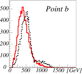
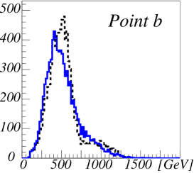
Figure 1: Various parton level $m^{\rm sub}_{T2}$ distributions at point b. The left plot, a solid line: the $m_{T2}^{\rm sub}$ distribution. The right plot, a solid line: a $\tilde{m}^{sub}_{T2}$ distribution, which is a $m_{T2}$ variables but calculated after subtracting the highest $p_{T}$ object from the hemisphere momenta. Dotted lines, $m^{\rm sub}_{T2}({\rm true})$ distributions, which uses generator information for the hemisphere assignment. Arbitrary normalizations are used for the $y$-axes. See text for details.

The endpoint at the gluino mass is more clearly visible for the $m^{\rm sub}_{T2}$ than for the $\tilde{m}^{\rm sub}_{T2}$ distribution. The improvement in $m^{\rm sub}_{T2}$ distribution may be explained as follows. At point b, a parton from $\tilde{q}\rightarrow q\tilde{g}$ has a large open angle to the gluino decay products on average. The event effectively has three axes: the two momenta of the two gluino decay products and the momentum of the extra parton from squark decay. The assumption of the hemisphere algorithm that events must have two axes may lead to an incorrect hemisphere assignment. Removing the highest $p_{T}$ parton before the hemisphere assignment therefore makes the kinetic endpoints more visible.

The successful endpoint reconstruction shows that the hemisphere algorithm reconstructs a total visible momentum of a squark/gluino decay more or less correctly. One can check this explicitly by counting the number of partons assigned to an incorrect hemisphere. (Fig. 2). The solid (dashed) histograms correspond to the distributions of the number of mis-reconstructed partons for the case that the highest $p_{T}$ parton is removed before (after) the hemisphere assignment. The improvement achieved by removing the highest $p_{T}$ parton before the hemisphere assignment is clearly seen at point a (the left plot). At this point, $m_{\tilde{q}}=1516$ GeV and $m_{\tilde{b}}=796$ GeV, so the parton from the squark decay should have $p_{T}$ of the order of several hundred GeV. We also see mild improvement at point b (the middle plot). At point e (the right plot), the squark and gluino masses are close, $(m_{\tilde{q}}-m_{\tilde{g}})/m_{\tilde{g}}=0.36$. In this case, removing the highest $p_{T}$ jet before the hemisphere assignment leads to the slightly worse reconstruction efficiency. The number of mis-reconstructed partons is either 0 or one for more than half of the events in Fig. 2.

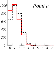
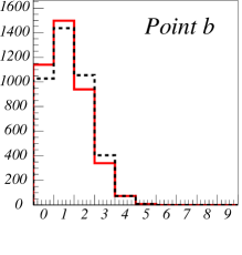
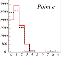
Figure 2: The distributions of the number of partons assigned to an incorrect hemisphere at point a (left), b (middle) and e (right). In all figures, solid (dashed) histograms correspond to the case that the highest $p_{T}$ parton is removed before (after) the hemisphere assignment. Arbitrary normalizations are used for the $y$-axes. See text for details.

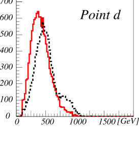
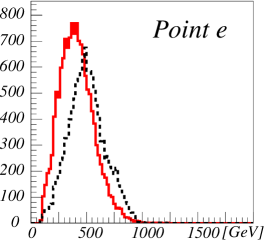
Figure 3: The $m^{\rm sub}_{T2}$ distributions (solid) and the $m^{\rm sub}_{T2}({\rm true})$ distributions (dashed) for squark-gluino co-production events at points d and e. Arbitrary normalizations are used for the $y$-axes.

If the highest $p_{T}$ parton does not arise from $\tilde{q}$ decay, the gluino endpoint cannot be reconstructed even for squark-gluino production events. The probability strongly depends on the model parameters. In Fig. 3 we show the $m^{\rm sub}_{T2}$ distributions for only squark-gluino co-production events at points d (left) and e (right). The gluino endpoint can be seen around 750 GeV from the $m_{T2}^{\rm sub}$ distribution at point d, which is close to that of the $m_{T2}^{\rm sub}({\rm true})$ distribution shown in the dotted line. However, at point e, even in the $m_{T2}^{\rm sub}({\rm true})$ distribution we cannot see the clear structure at the gluino mass.

The difference between the $m_{T2}^{\rm sub}$ and $m_{T2}^{\rm sub}({\rm true})$ distributions at points d and e may be explained as follows. At point d, $(m_{\tilde{q}}-m_{\tilde{g}})/m_{\tilde{g}}=0.52$, and the energy of the parton from the squark decay is bigger than that from the gluino on average. This is why $m^{\rm sub}_{T2}$ shows clear gluino endpoints at point d. In contrast, $(m_{\tilde{q}}-m_{\tilde{g}})/m_{\tilde{g}}=0.36$ at point e. The $m_{\tilde{q}}-m_{\tilde{g}}$ is not large enough, and it is not likely that the parton from $\tilde{q}\rightarrow\tilde{g}q$ has significantly high $p_{T}$ compared with those coming from the gluino decays. This is why the $m^{\rm sub}_{T2}({\rm true})$ distribution does not show the endpoint at the gluino mass, it could be a problem to extract the gluino mass from the $m^{\rm sub}_{T2}$ distribution. However, the $m_{T2}^{\rm sub}$ distribution of $\tilde{q}\tilde{g}$ production is significantly smeared towards the lower $m_{T2}$ value. In the actual situation, the contribution from gluino-gluino pair productions would be added, and the $m_{T2}^{\rm sub}$ distribution would have the endpoint at the gluino mass. We will see in the next section that the contamination from squark-gluino production is not serious.

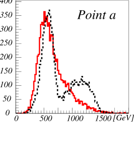
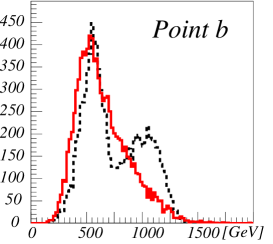
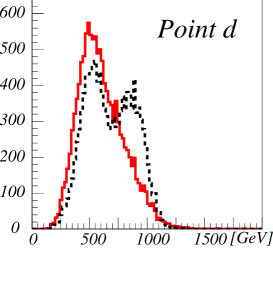
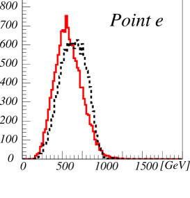
Figure 4: The parton level $m_{T2}$ distributions at points a, b, d and e. The solid lines correspond to the distributions using the hemisphere algorithm, while the dotted lines correspond to those with correct parton assignments obtained by using the generator information. Arbitrary normalizations are used for the $y$-axes.

For completeness, we show the parton level $m_{T2}$ distributions at points a, b, d and e in Fig. 4 to emphasize the difference between $m_{T2}$ and $m^{\rm sub}_{T2}$ distributions. The solid histograms are the $m_{T2}$ distributions using the hemisphere algorithm, while the dotted histograms correspond to the $m_{T2}({\rm true})$ distributions which are obtained by assigning the partons arising from a parent particle $i$ to hemisphere $i$ using generator information. At points a, b and d, the $m_{T2}({\rm true})$ distribution has two peaks. The peak at the lower $m_{T2}$ value comes from gluino-gluino production, while the peak at higher $m_{T2}$ corresponds to the squark-gluino and squark-squark productions. The endpoint of the distributions coincides with squark mass. The double peak structure cannot be seen in the distributions of $m_{T2}$, but the endpoints are the same as that of $m_{T2}({\rm true})$.

The slope of the distribution near the endpoint becomes flatter with increasing squark mass as can be seen from the distributions at points a, b, and d. In particular, the existence of a high $p_{T}$ parton from squark decay leads to some confusions in the hemisphere algorithm at point a, and a careful study of the distribution would be required to extract the squark mass from the fit. The peak of the $m_{T2}$ distribution coincides with the lower $m_{T2}({\rm true})$ peak. The events near the peak come from gluino pair productions at points a, b, and d. In principle, the position of the peak contains the gluino mass information. However, this is not easy to observe because the SM background may also be large in this region. At point e, although the endpoints of the $m_{T2}$ and $m_{T2}({\rm true})$ distributions are consistent, the squark and gluino masses are too close for the two peak structure to be seen.

3 The MC simulation of the signal

We have shown that the endpoints of $m_{T2}$ and $m_{T2}^{\rm sub}$ distributions carry the information on squark and gluino masses using parton level events. In this section we study the events produced by a parton shower Monte Carlo HERWIG (in the particle level) with a detector simulator AcerDET under the set of cuts to reduce the standard model backgrounds. The simple snowmass cone algorithm implemented in AcerDET is used for finding jets and we set the cone size $R=0.4$.

Figure 5: The inclusive $m_{T2}$ destributions at points a b, d and f (from left to right). The up squark mass is 1516, 1342, 1175, 881 GeV from left to right, respectively. Unit of $y$-axes is events/bin/$1\,$fb^-1.

Figure 6: The fitted $m_{T2}$ and $m_{T2}^{sub}$ endpoints (solid lines) and $m_{\tilde{q}}$ and $m_{\tilde{g}}$ (dashed lines) at each model point. The bars show the size of statistical errors for 50,000 SUSY events.

We apply the following cuts to the events.

• Jet $p_{T}$ cuts: $n_{50}\equiv N_{\rm jet}(p_{T}>50~{}{\rm GeV})\geq 4$, $n_{100}\equiv N_{\rm jet}(p_{T}>100~{}{\rm GeV})\geq 1$.

• $M_{\rm eff}(\equiv\sum_{p^{\rm jet}_{T}>50{\rm GeV}}p_{T}+E\!\!\!/_{T})>500$ GeV

• Transverse sphericity: $S_{T}>$ 0.2.

• Missing Transverse momentum:$E\!\!\!/_{T}>200$ GeV, $E\!\!\!/_{T}>0.2M_{\rm eff}$.

• No isolated lepton with $p_{T}>20$ GeV.

These cuts are similar to the standard SUSY cuts in the ATLAS TDR [6], except for our tighter $E\!\!\!/_{T}$ cut. We veto events with isolated leptons because a hard lepton might be assoicated with a hard neutrino. If there is a hard neutrino in an event, $p_{\rm Tmiss}$ of the event may not be the sum of the transverse momenta of LSPs. In that case, the endpoint of the $m_{T2}$ distribution might be smeared.

We first show the $m_{T2}$ distributions for our model points. The $m_{T2}$ distributions for $m_{\rm test}=10$ GeV under the SUSY cuts are shown in Fig. 5. For each point, we have generated 50,000 SUSY events and the distribution is scaled to correspond to $\int dt{\cal L}=1\,$fb^-1 of luminosity.

The endpoint of the $m_{T2}$ distribution is roughly at $\sim m_{\tilde{q}}$. We fit the distributions to linear functions

$$f(m) = a(m-m^{\rm end}_{T2})+c\ \ ({\rm for}\ \ m<m^{\rm end}_{T2})$$ (6)

$$= b(m-m^{\rm end}_{T2})+c\ \ ({\rm for}\ \ m>m^{\rm end}_{T2}),$$ (7)

and the fitted $m^{\rm end}_{T2}$ values are shown in Fig. 6. Here, the statistical errors shown in bars correspond to 50,000 total SUSY events. The obtained $m_{T2}^{\rm end}$ and $m_{\tilde{q}}$ are consistent except at points a and f. For point f, the squark and gluino masses are too close, and it is natural that the endpoint fall at weighted mean of gluino and squark masses. For point a, due to the very large mass difference between squark and gluino, the hemisphere method involving the highest $p_{T}$ jet does not work perfectly.

Note that there is some ambiguity in choosing a fitting region. For example, for point a, the distribution consists of the two components, one arising from the gluino-gluino production with the endpoint around $800\,$GeV and the other from the squark-gluino production with the endpoint around $1400\,$GeV. We fit the distribution above $m_{T2}>1000\,$GeV for this point. If we did the same fit at point f (the right plot), we might fit the mis-reconstructed tail of the events and therefore might obtain the endpoint at $1150\,$GeV. This suggests that the region of the fit must be chosen carefully. In particular, the events near the fitted endpoint must make up a sizable fraction of the total events. For points b, d and f, we first fit the region from the $m_{T2}$ slightly above the peak position of the distribution up to the highest bin with enough statistics ($>10$ events/bin). We then increase the lower limit until we obtain a small $\Delta\chi^{2}$. The $\Delta\chi^{2}/{\rm n.d.f}$ is less than 1 except at points c and e, and all fits satisfy $\Delta\chi^{2}/{\rm n.d.f}<2$.

Figure 7: The $p_{T}$ distributions of the highest $p_{T}$ jet (left) among the jets with $|\eta|<3$, and the distributions of the $m^{\rm sub}_{T2}$ (right) at point a. The dashed lines show the contributions from the events with $n_{300}=1$ and the dotted lines show the contributions from the events with $n_{\tilde{q}}=1$. The standard SUSY cuts are applied for all plots, and $m_{\rm test}=10$ GeV. Unit of $y$-axes is events/bin/$1\,$fb^-1.

Figure 8: The same as Fig. 7 but at point f.

Figure 9: The $m^{\rm sub}_{T2}$ destributions at points a to f normalized for $1\,$fb^-1. The input gluino masses differ slightly among the model points as we fix gaugino mass at the GUT scale. The top figures correspond to points a, b and c from left to right, and $m_{\tilde{g}}=796,785$, and 780 GeV respectively. The bottom figures correspond to points d, e and f, and $m_{\tilde{g}}=773,762$ and 745 GeV. The squark mass is 1516 GeV at point a and 881 GeV at point f.

We now demonstrate the gluino mass determination using the endpoint of the $m^{\rm sub}_{T2}$ distribution. Here we must pay some attention to reduce the contributions from the squark-squark pair productions, which give the endpoints of the $m^{\rm sub}_{T2}$ distribution as $m_{\tilde{q}}$. This contribution smears the endpoint at the gluino mass. It is important to find the cuts to reduce the events.

We find that the cut on the number of high $p_{T}$ jets above a certain threshold is useful to reduce the contamination, becuase the squark decay tends to give high $p_{T}$ jets, as we have discussed earlier. To see this, we first show the distributions of the highest $p_{T}$ jet at point a for 50,000 generated events in Fig. 7. The solid lines show the $p_{T}(1st)$ distribution, where $p(1st)$ is the momentum of the highest $p_{T}$ jet among the jets with $|\eta|<3$. The dashed lines show the contribution from the events with $n_{300}\equiv N_{\rm jet}(p_{T}>300$ GeV$,|\eta|<3)=1$ and the dotted lines show the contributions of the events with $n_{\tilde{q}}=1$, where $n_{\tilde{q}}$ is the number of primary produced 1st generation squarks of the events. The standard SUSY cuts are applied to the events. We can see that most of the events with $p_{T}(1st)>300$ GeV satisfy $n_{300}=1$ and they mostly come from squark-gluino productions. Therefore, if $n_{300}\geq 2$, they are likely come from squark-squark pair production events.

Based on the above observation, we calculate the $m^{\rm sub}_{T2}$ distribution only for the events which have only one or zero high $p_{T}$ jet above a certain $p_{T}$ threshold. The actual value of the $p_{T}$ cut should be chosen based on the signal distribution. For our model points, we take the cut $n_{300}\leq 1$. We do not include the events with $n_{300}\geq 2$, because our MC simulations show that they mostly come from the squark pair production. In the right figure, we show $m_{T2}^{\rm sub}$ distributions for the events $n_{300}=1$ at point a. The dotted line shows the distribution with $n_{300}=1$ and $n_{\tilde{q}}=1$. The dashed line is the distribution with $m_{T2}>800$ GeV, $n_{300}=1$ and $n_{\tilde{q}}=1$. All distributions show the $m_{T2}^{\rm sub}$ endpoint close to the gluino mass value $\sim 800$ GeV, which is expected from the parton level analysis.

Fig. 8 shows the same distributions at point f. Events from squark-gluino co-production still dominate the events with $p_{T}>300$ GeV, and a significant fraction of the events satisfy $n_{300}=1$. The events near the $m^{\rm sub}_{T2}$ endpoint mostly come from squark-gluino production. The endpoint of the distribution $\sim 750$ GeV is consistent with the gluino mass.

The $m_{T2}^{\rm sub}$ distributions at points a to f for $1\,$fb^-1 of integrated luminosity are shown in Fig. 9. Here we require $n_{300}\leq 1$; therefore, the distributions now include significant events from gluino-gluino production unlike the previous plots. We have seen that the $m_{T2}$ distribution changes significantly among points a to f. The $m_{T2}^{\rm sub}$ distributions are, by contrast, similar. This is because the $m^{\rm sub}_{T2}$ endpoints must be very close to the true gluino mass $m_{\tilde{g}}\sim 750$ GeV (up to the difference of the test LSP mass from the true LSP mass). This is also seen in Fig. 6, where the value of the fitted $m^{\rm sub}_{T2}$ endpoint is shown together with the gluino mass for each point.

4 Background $m_{T2}$ and $m^{\rm sub}_{T2}$ distributions

The Standard Model background to the SUSY processes has been studied by ATLAS and CMS groups extensively. The ratio $E\!\!\!/_{T}$ $/M_{\rm eff}$ gives a good discrimination between the SUSY signal and the background. In the previous section we required $E\!\!\!/_{T}/M_{\rm eff}>0.2$ in addition to $M_{\rm eff}>500$ GeV and $E\!\!\!/_{T}>200$ GeV.

The production cross section of the SM background is huge compared with the typical signal cross section. To measure the endpoint of the signal $m_{T2}$ and $m^{\rm sub}_{T2}$ distributions, the signal to noise ratio ($S/N$) must be sufficiently small near the endpoint. The SM backgrounds in the 0-lepton channel after the standard SUSY cuts come from the four different sources: $t\bar{t}$, $W^{\pm}$, $Z^{0}$ productions with multiple jets, and QCD multi-jet processes. Bottom quark productions and the mis-measurements of particle energies can give the missing energy to QCD multi-jet processes. It is difficult to estimate the QCD background without knowing detector performances in detail. We therefore do not attempt to do so in this paper. In recent ATLAS and CMS studies [17], the four channels contribute to the background at roughly the same order of magnitude after the cuts to reduce the SM backgrounds, although QCD background decreases much faster with increasing $M_{\rm eff}$.

	$t\bar{t}$	$W$	$Z$	total
$m_{T2}>500$ GeV	77.7	104.9	107.0	289.6
	38.4	44.8	39.9	123.1
$m_{T2}>700$ GeV	20.3	24.4	23.4	68.2
	10.0	12.0	10.4	32.4
$m_{T2}^{\rm sub}>300$ GeV	90.3	80.4	82.2	252.9
	44.2	38.5	31.7	113.1
$m_{T2}^{\rm sub}>500$ GeV	11.1	6.9	6.1	24.0
	8.1	4.9	3.8	16.8
luminosity	13.1 fb-1	13.5 fb-1	19.1 fb-1

Table 3: Number of SM background events per $1\,$fb^-1. For each row, upper (lower) numbers correspond to the events without (with) a cut on the hemisphere masses, $m_{\rm hemi}>200$ GeV. The last row shows the number of generated events for this study in terms of the corresponding integrated luminosity.

The source of missing $E_{T}$ for the processes $t\bar{t}$, $Z^{0}$, and $W^{\pm}+n$ jets is primarily escaping neutrinos, and missing $E_{T}$ arising from energy mis-measurements is less important. We generate these events using ALPGEN [28, 29], and parton shower and initial state radiations are estimated by interfacing the parton level events to HERWIG. We generate $Z^{0}(\rightarrow\nu\bar{\nu})+n$ jets for $n\leq 5$ , $W^{\pm}(\rightarrow l\nu)+n$ jets ($n\leq 4$) , and $t\bar{t}+n$ jets ($n\leq 2$) , so that tree level 0 lepton events have at least 4 or 5 jets including $\tau$ jets. We require minimum parton separation $\Delta R_{jj}>0.6$, and place a cut on the forward parton of $|\eta|<5$. The events are then matched so that there is no double counting between parton shower and hard partons by using the MLM matching scheme provided by ALPGEN. In this scheme, we generate the processes with up to $n_{max}$ parton. The events from the processes with $n$ partons ($n<n_{\rm max}$) are accepted only if jets and partons match ($n_{\rm jet}=n$), while the events from the processes with $n_{\rm max}$ partons are accepted if $n_{\rm jet}\geq n$. In order to reduce the number of produced events while keeping enough statistics for the kinematical region we are interested in, we require $\sum_{\rm parton}E_{T}>400$ GeV for $W$+ $n$ jets, $E\!\!\!/_{T}>150$ GeV for $Z+n$ jets, $\sum_{\rm parton}E_{T}>500$ GeV for $t\bar{t}$+ $n$ jets. The effect of additional jets on the signal distributions is small and discussed in Appendix A.2.

AcerDET performs Gaussian smearing for jet momenta, the missing momentum, and isolated lepton momenta. It does not contain various potentially important instrumental effects, such as non-Gaussian tails of the energy smearing and lepton inefficiencies. Therefore, our background estimate is given in this paper for illustrative purpose, and more realistic estimates must be performed by the experimental groups.

Keeping this in mind, Table 3 summarizes results of our event generations. The number of background events for $\int dt{\cal L}=1\,$fb^-1 under various cuts are given. The bottom row shows the corresponding luminosities we have generated for the background processes. We apply the SUSY cuts given in Section 4. In addition, we require $n_{300}\leq 1$ for $m_{T2}^{\rm sub}$ distribution. We do not include $K$ factors, as the corresponding higher order QCD corrections are not available. Note that K factors of $t\bar{t}$ production and SUSY production tend to cancel partially. For each row, upper (lower) numbers correspond to the events without (with) a cut on the hemisphere masses, $m_{\rm hemi}>200$ GeV. The background with the hemisphere mass cut is reduced by more than a factor of 2. This suggests that the background events are dominated by the configurations that a few jets are either soft or colinear to leading hard jets and therefore the masses of the hemispheres are small. The background distributions will be studied in detail elsewhere.

Figure 10: Signal and background distributions at point f (the top figures) and at point d (the bottom figures). Unit of $y$-axes is events/bin/$1\,$fb^-1.

Figure 11: The signal (solid) and background (dashed) distributions at point b. The bottom figures show the distributions with the hemisphere mass cut $m^{1(2)}_{\rm hemi}>200$ GeV. Unit of $y$-axes is events/bin/$1\,$fb^-1.

Fig. 10 shows the distribution of background, together with the signal distribution at points f (the top figures) and d (the bottom figures). These distributions are without hemisphere mass cuts. The signal is larger than the background above $m_{T2}>600$ $(750)$ GeV at points f (d) for the $m_{T2}$ distribution, which is much smaller than expected $m_{T2}^{\rm end}=m_{\tilde{q}}=881$ GeV ( $1175$ GeV). The endpoints of the signal $m_{T2}$ and $m^{\rm sub}_{T2}$ distributions may be extracted as a kink in the total distribution in this case. The signal and background distributions of $m_{T2}^{\rm sub}$ are also shown in the right plots. Again, the level of the background is small near the endpoint.

We also show the same distribution at point b in Fig. 11. The signal cross section involving $\tilde{q}$ production is reduced by a factor of $1/5$ from that at point f (See Table 2). The $S/N$ above $m_{T2}>700$ GeV is now $\sim 1$ and the cross point of the signal and the background is at $m_{T2}=800\,$GeV. By applying the hemisphere mass cut, we can reduce the background significantly. The improvement of $S/N$ near the endpoint can be seen by comparing the top and bottom figures without/with the hemisphere mass cut. It is important to reduce the background to measure the squark and gluino masses near the discovery regions.

5 Conclusions

The ATLAS and CMS experiments at the LHC can discover squarks and gluinos in the MSSM with masses less than 1.5 TeV at the early stage of the experiment with luminosity around $\int dt{\cal L}=1\,$fb^-1. Developing a reliable method of estimating squark and gluino masses with the discovery is an important step to study supersymmetry at the LHC.

For this purpose we cannot rely on the clean golden channels such as $l^{\pm}l^{\mp}+$ jets, becuase they tend to have small branching ratios and are sensitive to the model parameters. In a previous paper[22], we defined an inclusive $m_{T2}$ variable. This variable can be calculated for any event with jets and missing transverse energy. It is calculated in two steps; we first define the two hemisphere axes by assigning particles into the two leading jets of the events, then, the $m_{T2}$ variable is caluculated from the two hemisphere momenta and missing transverse energy. We pointed out that the endpoint of the $m_{T2}$ distribution is sensitive to the squark mass for the case $m_{\tilde{q}}>m_{\tilde{g}}$.

In this paper, we define a “sub-system” $m_{T2}$, $m^{\rm sub}_{T2}$. This is an $m_{T2}$ variable calculated without including the highest $p_{T}$ jets for the hemisphere assignments and $m_{T2}$ calculation. In the case that $m_{\tilde{q}}>m_{\tilde{g}}$ and the other sparticles are lighter, the endpoint of $m^{\rm sub}_{T2}$ distribution gives us information on $m_{\tilde{q}}$. In this paper, we show convincing evidence for sample model points within the reach for $\int dtL=1\,$fb^-1.

We also provide various parton level checks on the hemisphere algorithm. We estimate background distributions arising from $t\bar{t}$+$n$ jets, $Z^{0}$+ $n$ jets and $W^{\pm}$ + $n$ jets using ALPGEN and find out that $S/N$ ratio is large for the events near the $m_{T2}$ endpoints at our sample points. In the Appendix, we also provide a study of SUSY$+n$ jet distributions using MadGraph/MadEvent, and find that the endpoint is stable with the ME corrections.

Appendix A Appendix

A.1 The $m_{T2}$ endpoint for squark-gluino production events

In this Appendix, we show the condition for which the endpoint of the ideal $m_{T2}$ distribution for the squark-gluino production events coincides with the squark mass at $M_{\rm test}=m_{\rm LSP}$.

The squark-gluino $m_{T2}$ is calculated by minimizing $\max\{m_{T}^{(\tilde{q})},m_{T}^{(\tilde{g})}\}$ under the condition that the sum of transverse test momenta of two LSP is equal to the $E\!\!\!/_{T}$. It is known that the transverse mass $m_{T}^{(i)}$ ($i=\tilde{q},\tilde{g}$) as a function of the test LSP momentum has the global minimum, which is called the unconstrained minimum (UCM) [15]. There are cases where $m_{T2}$ is given by the unconstrained minimum of the transverse mass on one side $(m_{T}^{(i)})_{\rm UCM}$. This situation occurs when $m_{T}^{(j)}$ on the other side for the test LSP momentum which gives the $(m_{T}^{(i)})_{\rm UCM}$ is smaller than $(m_{T}^{(i)})_{\rm UCM}$.

In Ref.[18], it is shown that the UCM of the squark system ($(m_{T}^{(\tilde{q})})_{\rm UCM}$) is given by

$$(m^{(\tilde{q})}_{T})_{\rm UCM}=m^{(\tilde{q})}_{\rm vis}+M_{\rm test},$$ (8)

where $m^{(\tilde{q})}_{\rm vis}$ is the invariant mass of the visible particles from the squark decay. The maximum of $(m_{T}^{(\tilde{q})})_{\rm UCM}$ is, therefore, given by substituting the maximum of $m^{(\tilde{q})}_{\rm vis}$ into Eq.8. The maximum of the $m^{(\tilde{q})}_{\rm vis}$ is given by

$$(m^{(\tilde{q})}_{\rm vis})^{\rm max}=m_{\tilde{q}}-m_{\rm LSP},$$ (9)

if the LSP from squark decay can be at rest in the squark rest frame. In this case, the maximum of the UCM of the squark system can reach the squark mass at $M_{\rm test}=m_{\rm LSP}$, and the maximum of the squark-gluino $m_{T2}$ is identical to the squark mass at $M_{\rm test}=m_{\rm LSP}$.

Figure 12: A Kinematical configuration of squark decay

We now consider the condition that the LSP can be at rest in the squark rest frame. In the following discussion, we concentrate on the case that the squark decays into the gluino and a jet. The gluino from the squark subsequently decays into the visible objects and the LSP (See Fig. 12). The LSP momentum in the gluino rest frame ($p^{\prime}_{\rm LSP}$) depends on the invariant mass of the visible objects ($m^{(\tilde{g})}_{\rm vis}$) as

$$|p^{\prime}_{\rm LSP}|=\frac{1}{2m_{\tilde{g}}}\sqrt{m_{\tilde{g}}^{4}-2m^{2}_{\tilde{g}}((m^{(\tilde{g})}_{\rm vis})^{2}+m^{2}_{\rm LSP})+((m^{(\tilde{g})}_{\rm vis})^{2}-m^{2}_{\rm LSP})^{2}}~{}~{}.$$ (10)

If the LSP is produced in the opposite direction from the gluino momentum and the gluino velocity is not too large, the LSP can be at rest in the squark rest frame for a suitable value of the invariant mass of the visible objects ($\tilde{m}_{\rm vis}^{(\tilde{g})}$). In this situation, the LSP momentum in the squark rest frame ($p_{\rm LSP}$) is obtained by the Lorentz boost of the $p^{\prime}_{\rm LSP}$ as

$$p_{\rm LSP}=\gamma_{\tilde{g}}(-|\beta_{\tilde{g}}|E^{\prime}_{\rm LSP}+|p^{\prime}_{\rm LSP}|)~{},$$ (11)

where $E^{\prime}_{\rm LSP}$ is the energy of the LSP in the gluino rest frame, and the Lorentz boost factors $\beta_{\tilde{g}}$ and $\gamma_{\tilde{g}}$ are given by

$$|\beta_{\tilde{g}}|=\frac{m^{2}_{\tilde{q}}-m^{2}_{\tilde{g}}}{m^{2}_{\tilde{q}}+m^{2}_{\tilde{g}}},~{}~{}~{}~{}~{}\gamma_{\tilde{g}}=1/\sqrt{1-\beta^{2}_{\tilde{g}}}=\frac{m^{2}_{\tilde{q}}+m^{2}_{\tilde{g}}}{2m_{\tilde{q}}m_{\tilde{g}}}.$$ (12)

By solving the equation $p_{\rm LSP}=0$, we obtain

$$(\tilde{m}_{\rm vis}^{(\tilde{g})})^{2}=m_{\tilde{g}}^{2}\big{(}1-\frac{m_{\rm LSP}}{m_{\tilde{q}}}\big{)}\big{(}1-\frac{m_{\tilde{q}}m_{\rm LSP}}{m^{2}_{\tilde{g}}}\big{)}~{}.$$ (13)

Note that if $m_{\tilde{q}}m_{\rm LSP}>m^{2}_{\tilde{g}}$, the equation $p_{\rm LSP}=0$ does not have any solution for positive $\tilde{m}_{\rm vis}^{(\tilde{g})}$. In this case, the LSP cannot be at rest in the squark rest frame, and $(m^{(\tilde{q})}_{T})_{\rm UCM}$ is less than the squark mass. Even if the equation $p_{\rm LSP}=0$ has a solution for positive $\tilde{m}_{\rm vis}^{(\tilde{g})}$, there are cases where $m_{\rm vis}^{(\tilde{g})}$ has a non-vanishing kinematical lower bound due to a heavy standard model particle, such as $t$, $Z$ and $W$. If the lower bound is smaller than the solution $\tilde{m}_{\rm vis}^{(\tilde{g})}$, $(m^{(\tilde{q})}_{T})_{\rm UCM}$ cannot reach the squark mass. For our model points, the solution (13) is $\tilde{m}_{\rm vis}^{(\tilde{g})}/m_{\tilde{g}}=0.83$ for point a, and $\tilde{m}_{\rm vis}^{(\tilde{g})}/m_{\tilde{g}}=0.85$ for point f. On the other hand, the kinematically allowed range of the visible invariant mass is roughly $0.50\leq m_{\rm vis}^{(\tilde{g})}/m_{\tilde{g}}\leq 0.86$ for point a, and $0.55\leq m_{\rm vis}^{(\tilde{g})}/m_{\tilde{g}}\leq 0.86$ for point f. Therefore, the endpoint of the ideal $m_{T2}$ distribution in the squark-gluino production events is identical to the squark mass in our model points.

A.2 The effect of Matrix Element corrections to the signal distribution

In this appendix we consider the matching effect of multi-jet matrix elements (ME) and parton showers on the $m_{T2}$ distribution. When we calculate the signal $m_{T2}$ distributions in this text, we generate SUSY processes at the lowest-order hard process and then generate multi-jet events by parton showers. In general, there are ME corrections from hard parton emissions in the lowest order hard process, which may not be included in the parton shower approach. Note that we have applied cuts $p_{T}>50\,$GeV and $|\eta|<3$ for the jets to be included in the hemispheres. We need to check that this is enough to kill the effects of initial state radiations.

When the ME corrections are taken into account, we should avoid double counting of emissions in overlapping phase space and need some kind of matching scheme to merge the ME corrections. Here, we study the ME corrections using the MadGraph /MadEvent MC generator [33], in which the matching between the ME corrections and the parton showers is implemented. For our analysis, we use a modified MLM matching procedure with $k_{\perp}$ jets. In this scheme, the parton emissions are separated into two phase space regions at some $k_{\perp}$. In MadGraph/MadEvent, only events with enough separated partons, $k_{\perp}>$ xqcut, are generated after the matrix element simulation. Then parton showering is performed and the partons are clustered into jets using the $k_{\perp}$ algorithm. After this procedure, the matching between the jets and the partons from the matrix elements is performed using Pythia. If the distance between them is larger than Qcut, the event is discarded in order to avoid double counting.

In order to see the effect of the additional jet emission, we generate the SUSY events for the mSUGRA point SPS 1a using MadGraph/MadEvent. The generated parton level events are interfaced with Pythia to take into account the matching and the hadronization. We take the matching parameters as xqcut$=40~{}{\rm GeV}$, Qcut$=60~{}{\rm GeV}.$ After hadronic events are generated, we use AcerDET for detector simulations. We apply the same cuts given in the Sec. 4 to select the events.

In Fig. 13(a), we plot the $m_{T2}$ distributions for gluino pair-production processes with 0, 1, 2 jets. Since the total cross sections could receive large NLO corrections, the shape of $m_{T2}$ distribution is more important. For comparison, we normalize the each distribution to unity. We can see that the shapes of the $m_{T2}$ distributions are stable against the ME corrections. This is a good feature to obtain information on the gluino mass from the endpoint of the $m_{T2}$ distributions.

In Fig. 13(b) and 12(c), we plot the $m_{T2}$ distributions for squark pair-production (squark-gluino) processes with 0, 1 jet. We also normalize each distribution to unity. Again we can see that the $m_{T2}$ distributions are rather insensitive to the ME corrections and the matching.

Figure 13: (a) $m_{T2}$ distributions for ${\tilde{g}}{\tilde{g}}$ +0 jet (dashed), 1 jet (solid) 2 jets (dotted). (b) $m_{T2}$ distributions for ${\tilde{q}}{\tilde{q}}$ +0 jet (solid), 1 jet (dashed). (c) $m_{T2}$ distributions for ${\tilde{g}}{\tilde{q}}$ +0 jet (solid), 1 jet (dashed). Here SUSY spectrum is assumed as SPS 1a.

References

- [1] H. P. Nilles, Phys. Rept. 110 (1984) 1.
- [2] H. E. Haber and G. L. Kane, Phys. Rept. 117 (1985) 75.
- [3] S. P. Martin, arXiv:hep-ph/9709356.
- [4] I. Hinchliffe, F. E. Paige, M. D. Shapiro, J. Soderqvist and W. Yao, Phys. Rev. D 55 (1997) 5520 [arXiv:hep-ph/9610544].
- [5] S. Abdullin et al. [CMS Collaboration], J. Phys. G 28 (2002) 469 [arXiv:hep-ph/9806366].
- [6] ATLAS Collaboration, “ATLAS detector and physic perrformance Technical Design Report,” CERN/LHCC 99-14/15 (1999).
- [7] H. Bachacou, I. Hinchliffe and F. E. Paige, Phys. Rev. D 62 (2000) 015009 [arXiv:hep-ph/9907518].
- [8] I. Hinchliffe and F. E. Paige, Phys. Rev. D 61 (2000) 095011 [arXiv:hep-ph/9907519].
- [9] B. C. Allanach, C. G. Lester, M. A. Parker and B. R. Webber, JHEP 0009 (2000) 004 [arXiv:hep-ph/0007009].
- [10] M. M. Nojiri, G. Polesello and D. R. Tovey, arXiv:hep-ph/0312317.
- [11] K. Kawagoe, M. M. Nojiri and G. Polesello, Phys. Rev. D 71, 035008 (2005) [arXiv:hep-ph/0410160].
- [12] M. M. Nojiri, G. Polesello and D. R. Tovey, JHEP 0805, 014 (2008) [arXiv:0712.2718 [hep-ph]].
- [13] H. C. Cheng, D. Engelhardt, J. F. Gunion, Z. Han and B. McElrath, Phys. Rev. Lett. 100, 252001 (2008) [arXiv:0802.4290 [hep-ph]].
- [14] C. G. Lester and D. J. Summers, Phys. Lett. B 463 (1999) 99 [arXiv:hep-ph/9906349].
- [15] A. Barr, C. Lester and P. Stephens, J. Phys. G 29 (2003) 2343 [arXiv:hep-ph/0304226].
- [16] G. Weiglein et al. [LHC/LC Study Group], Phys. Rept. 426, 47 (2006) [arXiv:hep-ph/0410364].
- [17] Oleg Brandt, talk in Hadron Collider Physics Symposium 2008(HCP)
- [18] W. S. Cho, K. Choi, Y. G. Kim and C. B. Park, arXiv:0709.0288 [hep-ph]
- [19] B. Gripaios, arXiv:0709.2740 [hep-ph].
- [20] A. J. Barr, B. Gripaios and C. G. Lester, arXiv:0711.4008 [hep-ph].
- [21] W. S. Cho, K. Choi, Y. G. Kim and C. B. Park, arXiv:0711.4526 [hep-ph].
- [22] M. M. Nojiri, Y. Shimizu, S. Okada and K. Kawagoe, JHEP 0806, 035 (2008) [arXiv:0802.2412 [hep-ph]].
- [23] A. J. Barr, G. G. Ross and M. Serna, arXiv:0806.3224 [hep-ph].
- [24] D. R. Tovey, JHEP 0804, 034 (2008) [arXiv:0802.2879 [hep-ph]].
- [25] F. Moortgat and L. Pape, CMS Physics TDR, Vol. II, Report No. CERN-LHCC-2006, Chap. 13.4, p410
- [26] S. Matsumoto, M. M. Nojiri and D. Nomura, Phys. Rev. D 75 (2007) 055006 [arXiv:hep-ph/0612249].
- [27] J. Hubisz, J. Lykken, M. Pierini and M. Spiropulu, arXiv:0805.2398 [hep-ph].
- [28] M. L. Mangano, M. Moretti, F. Piccinini, R. Pittau and A. D. Polosa, JHEP 0307, 001 (2003) [arXiv:hep-ph/0206293].
- [29] M. L. Mangano, M. Moretti and R. Pittau, Nucl. Phys. B 632, 343 (2002) [arXiv:hep-ph/0108069].
- [30] T. Plehn, D. Rainwater and P. Skands, Phys. Lett. B 645, 217 (2007) [arXiv:hep-ph/0510144].
- [31] Johan Alwall, talk in ”The 16th International Confernce on Supersymmetry and the Unification of Fundamental Interactions. ” (SUSY08)
- [32] J. Alwall, M. P. Le, M. Lisanti and J. G. Wacker, arXiv:0803.0019 [hep-ph].
- [33] J. Alwall et al., JHEP 0709, 028 (2007) [arXiv:0706.2334 [hep-ph]].
- [34] G. Corcella et al., JHEP 0101 (2001) 010 [arXiv:hep-ph/0011363]; arXiv:hep-ph/0210213.
- [35] E. Richter-Was, arXiv:hep-ph/0207355.
- [36] M. Drees, Y. G. Kim, M. M. Nojiri, D. Toya, K. Hasuko and T. Kobayashi, Phys. Rev. D 63, 035008 (2001) [arXiv:hep-ph/0007202].
- [37] J. R. Ellis, K. A. Olive and Y. Santoso, Phys. Lett. B 539, 107 (2002) [arXiv:hep-ph/0204192].
- [38] J. R. Ellis, T. Falk, K. A. Olive and Y. Santoso, Nucl. Phys. B 652, 259 (2003) [arXiv:hep-ph/0210205].
- [39] F. E. Paige, S. D. Protopopescu, H. Baer and X. Tata, arXiv:hep-ph/0312045.
- [40] http://www.hep.phy.cam.ac.uk/ richardn/HERWIG/ISAWIG/