Quantum interference and spin-charge separation
in a disordered Luttinger liquid

Abstract

We study the influence of spin on the quantum interference of interacting electrons in a single-channel disordered quantum wire within the framework of the Luttinger liquid (LL) model. The nature of the electron interference in a spinful LL is particularly nontrivial because the elementary bosonic excitations that carry charge and spin propagate with different velocities. We extend the functional bosonization approach to treat the fermionic and bosonic degrees of freedom in a disordered spinful LL on an equal footing. We analyze the effect of spin-charge separation at finite temperature both on the spectral properties of single-particle fermionic excitations and on the conductivity of a disordered quantum wire. We demonstrate that the notion of weak localization, related to the interference of multiple-scattered electron waves and their decoherence due to electron-electron scattering, remains applicable to the spin-charge separated system. The relevant dephasing length, governed by the interplay of electron-electron interaction and spin-charge separation, is found to be parametrically shorter than in a spinless LL. We calculate both the quantum (weak localization) and classical (memory effect) corrections to the conductivity of a disordered spinful LL. The classical correction is shown to dominate in the limit of high temperature.

I Introduction

Interacting electrons in one dimension (1D) are a paradigmatic example of the strongly correlated fermionic systems. Electron-electron (e-e) interactions drive the 1D system into a non-Fermi liquid state known as the Luttinger liquid (LL) (for review see, e.g., Refs. sol79, ; voit94, ; schulz95, ; gog98, ; schulz00, ; maslov, ; giam04, ). In recent years, progress in nanofabrication technologies has made it possible to manufacture a variety of single- and few-channel quantum wires connected to the electric leads and to perform systematic transport measurements on the very narrow wires. The latter include single–wall carbon nanotubes nano1 ; nano2 ; nano3 ; nano4 ; nano5 ; nano6 ; nano7 , semiconductor-basedsemicond1 ; semicond2 ; Jompol ; Hew08 and metallicmetallic quantum wires, polymer nanofiberspolymer , as well as quantum Hall edge states.QHedge ; grayson05 The LL nature of these strongly correlated quantum wires has been supported by a wealth of experimental findings.nano1 ; nano2 ; nano3 ; nano4 ; nano5 ; nano6 ; nano7 ; semicond1 ; semicond2 ; metallic ; polymer ; QHedge ; grayson05 Another class of strongly-correlated quantum wires that has recently attracted a lot of interest is ultracold atomic gases confined to 1D geometry, for review see Ref. bloch08, .

Mesoscopic physics of strongly correlated electrons is one of the most important and promising directions of current research on 1D electron systems. Recent transport measurements on carbon nanotubesmorpurgo reported both sample-dependent conductance fluctuations and strong magnetoconductivity, in qualitative similarity to the mesoscopic phenomena in higher-dimensional disordered electron systems. In Ref. morpurgo, , the sample size $\sim 1\>\mu$m was of the order of the mean free path limited by impurity scattering. Electron transport through the nanotubes displayed, therefore, features characteristic of the crossover from ballistic conduction to a disorder-dominated regime. On the other hand, in the past few years techniques to grow nanotubes of size up to the millimeter scaleli04 ; purewal07 —much larger than the typical value of the disorder-induced mean free path—have been developed. First transport measurementsli04 ; purewal07 on the ultralong nanotubes provided evidence for disorder-induced diffusive motion of electrons in a wide range of temperature. Altogether, these advances have paved the way for systematic experimental study of interference-induced localization phenomena in 1D.

The theory of weak localization (WL) in a disordered LL of spinless electrons was developed in Refs. GMPlett, and GMP, (for recent advances in the ballistic $\sigma$-model framework, see also Ref. micklitz08, ). In the limit of weak interaction between electrons, the phase breaking length $l_{\phi}$ that sets up the infrared cutoff of WL was shown to obey $l_{\phi}\sim\alpha^{-1}(l_{T}l)^{1/2}$, where $\alpha\ll 1$ is the dimensionless interaction constant, $l_{T}\sim v/T$ the thermal length, $v$ the Fermi velocity, $T$ the temperature, $l$ the elastic mean free path. At sufficiently high temperatures, when $l_{\phi}\ll l$, the system is in the WL regime.SL The WL correction $\Delta\sigma_{\rm WL}$ to the Drude conductivity $\sigma_{\rm D}$ behaves then as $\Delta\sigma_{\rm WL}/\sigma_{\rm D}\sim\,-(l_{\phi}/l)^{2}\ln(l/l_{\phi})\sim-\alpha^{-2}(l_{T}/l)\ln(\alpha^{2}l/l_{T})$. Note that the WL dephasing length of spinless electrons originates from the interplay of interaction and disorder: both ingredients are necessary to establish a nonzero dephasing rate. As a result, $l_{\phi}$ in the WL regime is much longer than the total decay length of fermionic excitations $l_{ee}\sim\alpha^{-2}l_{T}$. The latter is the dephasing length relevant to the damping of Aharonov-Bohm oscillationsGMPlett ; GMP ; lehur02 ; lehur06 and to the smearing of a zero-bias anomaly in the tunnelling density of states.gutman08

In a spinful LL, the most prominent spin-related manifestation of non-Fermi liquid physics is a phenomenon of spin-charge separation (SCS) (see, e.g., Refs. sol79, ; voit94, ; schulz95, ; gog98, ; schulz00, ; maslov, ; giam04, ). The essence of the SCS in the LL model is that the spin and charge sectors of the theory in a bosonic representation are completely decoupled from each other and characterized by different interaction coupling constants. Correspondingly, the elementary bosonic excitations carrying spin and charge propagate with different velocities, independently of each other. Experimentally, the effect of the SCS on the spectral properties of a LL (as measured in electron tunnelling experiments) has been studied in Refs. semicond1, ; Jompol, . In the last few years, much attention has been given to the so-called “spin-incoherent regime” fiete07 in 1D systems with strongly different spin and charge velocities.matveev04 ; fiete04 ; cheianov04 For recent transport measurements in ballistic quantum wires which show signatures of the spin-incoherent behavior, see Ref. Hew08, and references therein.

While the difference in the spectral properties of spin and charge collective modes is not at all specific to 1D and is also characteristic of higher-dimensional Fermi liquids,baym04 the peculiarity of 1D is that the “factorization” of the bosonic modes modifies the single-particle fermionic properties in an essential way.footnote1 Our purpose is to investigate how the SCS affects the quantum interference phenomena in a disordered LL. In particular, we analyze the dynamical properties of fermionic excitations at finite temperature and employ the results of this analysis to calculate the WL correction to the conductivity of a spinful LL. The problem is rather nontrivial conceptually since the spin and charge degrees of freedom that constitute the electron in a LL acquire different velocities and the very notion of a specific quasiclassical electron trajectory characterized by a certain velocity—conventionally invoked in a description of WL—becomes ambiguous.

We show below that, despite the intricate nature of a single-electron motion in a spinful LL, the basic notions of WL remain applicable even when the SCS is incorporated in the calculation. However, the spin degree of freedom has dramatic consequences for the effects of e-e scattering. Most importantly, the decay rate of fermionic excitations is strongly enhanced in the presence of spin: the single-particle length $l_{ee}\sim\alpha^{-1}l_{T}$ becomes parametrically shorter than for spinless (spin-polarized) electrons. Moreover, in contrast to the spinless case, the WL dephasing length $l_{\phi}\sim\alpha^{-1}l_{T}$ becomes of the order of $l_{ee}$. As a result, also the WL dephasing turns out to be much stronger than without the SCS being included. The temperature at which spinful electrons get strongly localized ($l_{T}/l\sim\alpha$) is therefore much lower (for small $\alpha$) than for spinless electrons. Furthermore, we find that the WL correction to the conductivity is given by $\Delta\sigma_{\rm WL}/\sigma_{D}\sim-(l_{\phi}/l)^{2}\sim-\alpha^{-2}(l_{T}/l)^{2}$, showing a much faster temperature dependence of $\Delta\sigma_{\rm WL}$ than in the spinless case.

We also demonstrate that a classical “memory effect” (ME) in the electron scattering off disorder contributes to the $T$ dependence of the conductivity. Moreover, it gives the leading (larger than $\Delta\sigma_{\rm WL}$) correction to the Drude conductivity in the limit of high $T$. The obtained ME contribution $\Delta\sigma_{\rm ME}/\sigma_{D}\sim-l_{T}/l$ is essentially not related to e-e interactions and exceeds $\Delta\sigma_{\rm WL}$ only when the latter is sufficiently suppressed by the interaction-induced dephasing. Specifically, $|\Delta\sigma_{\rm ME}|\gg|\Delta\sigma_{\rm WL}|$ for $l_{T}/l\ll\alpha^{2}$ (i.e., for $l_{\phi}/l\ll\alpha$). Otherwise, $|\Delta\sigma_{\rm WL}|\gg|\Delta\sigma_{\rm ME}|$. Technically, the ME manifests itself in the same set of Feynman diagrams for the conductivity as the WL, so that we actually treat the two effects—the essentially classical ME and the essentially quantum WL—on an equal footing. What distinguishes them from each other is that the main contributions to $\Delta\sigma_{\rm WL}$ and $\Delta\sigma_{\rm ME}$ come from scattering on different impurity configurations. The WL correction stems from scattering on rare, compact three-impurity complexes in which the characteristic distance between all three impurities is of the order of the single-particle length $l_{ee}$. The ME correction is associated with impurity configurations in which two of impurities are located very close to each other, with a characteristic distance between them of the order of the thermal length $l_{T}$.

The remainder of the paper is organized as follows. In Sec. II we formulate the model of a disordered LL, discuss the basic physics of the SCS relevant to the e-e scattering, and describe the method of functional bosonization used in our calculation. Section III is devoted to an analysis of the spectral properties of fermionic excitations in various representations; in particular, in a “space-energy representation” employed for the calculation of the conductivity. In Secs. IV and V we evaluate the WL and ME corrections to the conductivity, respectively, by means of the functional bosonization method. In Sec. VI we present a complementary analysis based on the more conventional path-integral approach. Our results are summarized in Sec. VII.

II Model and method

We begin by formulating the model of a disordered spinful LL in Sec. II.1. In Sec. II.2 we present a simple argument which demonstrates the peculiarity of 1D geometry in that the spin degree of freedom affects the rate of e-e scattering in the LL in a crucial way. Section II.3 is devoted to an overview of the functional bosonization method.

II.1 Disordered Luttinger liquid

Throughout the paper we consider a single-channel infinite quantum wire. Linearizing the dispersion relation of electrons about two Fermi points at the wavevectors $k=\pm k_{F}$ with the velocity $v$, the Hamiltonian of a clean LL is written as ($\hbar=1$)

$$H_{\rm LL} = \sum_{k\mu\sigma}v(\mu k-k_{F})\Psi^{\dagger}_{\mu\sigma}(k)\Psi_{\mu\sigma}(k)$$

$$+ {1\over 2}\sum_{\mu\sigma\sigma^{\prime}}\int\!dx\,\big{(}n_{\mu\sigma}\,g_{4}\,n_{\mu\sigma^{\prime}}+n_{\mu\sigma}\,g_{2}\,n_{-\mu,\sigma^{\prime}}\big{)}~{}.$$

Here $\Psi_{\mu\sigma}(k)$ are the electron operators at the wavevector $k$, the index $\mu=\pm$ denotes two branches of chiral excitations (right and left movers), and $\sigma=\uparrow,\downarrow$ stands for two spin projections. The e-e interaction enters Eq. (LABEL:1) through the coupling constants $g_{4}$ and $g_{2}$. These describe forward e-e scattering with small momentum transfer (much smaller than $k_{F}$) between electrons from the same ($g_{4}$) or different ($g_{2}$) chiral branches. We assume that the e-e interaction is short-ranged and represent the interaction part of the Hamiltonian in terms of the local in space electron density operators $n_{\mu\sigma}(x)=\psi^{\dagger}_{\mu\sigma}(x)\psi_{\mu\sigma}(x)$. The parameters of the Hamiltonian with the linearized dispersion should be understood as effective (phenomenological) couplings of the low-energy theory, which include possible high-energy renormalization effects, similar to Fermi-liquid theory.

The LL Hamiltonian (LABEL:1) does not contain the term

$$H_{\rm bs}={1\over 2}\sum_{\mu\sigma\sigma^{\prime}}\int\!dx\,\psi^{\dagger}_{\mu\sigma}\psi_{-\mu,\sigma}\,g_{1}\,\psi^{\dagger}_{-\mu,\sigma^{\prime}}\psi_{\mu\sigma^{\prime}}~{},$$ (2.2)

which describes backward e-e scattering with large momentum transfer resulting in a change of chirality $\mu$. If one begins with a microscopic model of electrons interacting via a finite-range externally screened Coulomb potential, the constants $g_{2,4}$ in Eq. (LABEL:1) and $g_{1}$ in Eq. (2.2) are related to the Fourier transforms of this potential at zero and $2k_{F}$ momenta, respectively. The forward scattering dominates provided that the radius of external screening $d$ (e.g., the distance to a metallic gate) is much larger than $k_{F}^{-1}$. We assume that this is the case and neglect $H_{\rm bs}$ throughout the paper below.remark1 Treating the Coulomb potential in Eq. (LABEL:1) as short-ranged is legitimate for scattering processes with momentum transfer much smaller than $d^{-1}$. This same scale $d^{-1}$ fixes the ultraviolet momentum cutoff in our formulation of the low-energy theory.

The only source of electron backscattering in our model is thus a static random potential $U(x)$ due to the presence of impurities. We assume that fluctuations of $U(x)$ are Gaussian and characterized by the correlation function $\langle U(x)U(x^{\prime})\rangle=\delta(x-x^{\prime})v^{2}/2l_{0}$ (“white noise”). Here $l_{0}$ is the transport elastic mean free path in the absence of interaction. The disorder is considered to be weak, $k_{F}l_{0}\gg 1$. The disorder-induced backscattering term in the Hamiltonian is given by

$$H_{\rm imp}=\sum_{\sigma}\ \int\!dx\,\big{(}U_{b}^{*}\ \psi^{\dagger}_{+\sigma}\psi_{-\sigma}+U_{b}\ \psi^{\dagger}_{-\sigma}\psi_{+\sigma}\big{)}~{},$$ (2.3)

where the backscattering amplitudes $U_{b}(x)$ are correlated as $\langle U_{b}(x)U^{*}_{b}(x^{\prime})\rangle=\langle U(x)U(x^{\prime})\rangle$ and $\langle U_{b}(x)U_{b}(x^{\prime})\rangle=0$. Forward scattering off impurities can be gauged out in the calculation of the conductivityabrikosov78 ; giam04 and will therefore be neglected from the very beginning. The total Hamiltonian $H$ that defines our model of a disordered spinful LL is thus

$$H=H_{\rm LL}+H_{\rm imp}~{}.$$ (2.4)

Throughout the paper we consider a quantum wire with spin and chiral channels not separated spatially in the transverse direction, so that the constants $g_{2}=g_{4}\equiv g$ are spin-independent and equal to each other. The plasmon velocity $u$ for the spinful case then reads

$$u=v/K_{\rho}=v(1+2g/\pi v)^{1/2}~{},$$ (2.5)

with $K_{\rho}$ being the Luttinger constant in the charge sector, whereas the velocity of elementary spin excitations is equal to $v$. It is convenient to characterize the strength of e-e interaction by the dimensionless coupling constant GMP $\alpha=(1-K_{\rho}^{2})/(1+3K_{\rho}^{2})$, which in the limit of weak interaction $\alpha\ll 1$ is written as

$$\alpha\simeq(1-K_{\rho})/2\simeq g/2\pi v~{}.$$ (2.6)

II.2 Why spin matters

To qualitatively understand the nature of dephasing of fermionic excitations in a spinful LL, it is instructive to recall the perturbative expansionGMPlett ; maslov of the self-energy of the single-particle Green’s function in the limit of weak interaction $\alpha\ll 1$ and discuss the e-e scattering rate at the Golden-rule level, first in the absence of disorder. For the spinless case, such an analysis has been performed in Refs. GMPlett, ; GMP, , and lehur06, —see also Refs. lehur02, ; GMPlett, ; GMP, ; lehur06, and Refs. GMPlett, ; lehur06, for a closely related calculation of the temporal decay of the single-particle Green’s function for spinless and spinful electrons, respectively. Since the physics of dephasing is governed by inelastic e-e scattering, a natural first step is to calculate at lowest (second) order in $\alpha$ the e-e scattering rate $\tau_{ee}^{-1}$ given by the imaginary part of the self-energy.

The Golden-rule expression for the e-e collision rate reads

$$\frac{1}{\tau_{ee}^{\rm GR}(\varepsilon)}=\int\!d\omega d\varepsilon^{\prime}\,K(\omega)\left(f^{h}_{\varepsilon-\omega}f_{\varepsilon^{\prime}}f^{h}_{\varepsilon^{\prime}+\omega}+f_{\varepsilon-\omega}f^{h}_{\varepsilon^{\prime}}f_{\varepsilon^{\prime}+\omega}\right),$$ (2.7)

where

$$K(\omega)=\eta_{s}[\,K^{H}_{++}(\omega)+K^{H}_{+-}(\omega)\,]+K^{F}(\omega)$$ (2.8)

is the kernel of the e-e collision integral and $f_{\varepsilon}$ is the Fermi distribution function, $f^{h}_{\varepsilon}=1-f_{\varepsilon}$. In Eq. (2.8), the Hartree terms $K^{H}_{++}\propto g_{4}^{2}$ and $K^{H}_{+-}\propto g_{2}^{2}$ are related to scattering of two electrons from the same $(++)$ or different $(+-)$ chiral branches, respectively, $K^{F}=-K^{H}_{++}$ is the exchange counterpart of $K^{H}_{++}$, $\eta_{s}$ is the spin degeneracy, $\eta_{s}=1$ for the spinless case and $\eta_{s}=2$ for the spinful case.

To order ${\cal O}(\alpha^{2})$, the Golden-rule scattering rate and the self-energy on the mass shell coincide with each other. At the Fermi level ($\varepsilon=0$) we have

$${1\over\tau_{ee}^{\rm GR}(0)}=-2\,\big{[}\,\eta_{s}({\rm Im}\Sigma^{H}_{++}+{\rm Im}\Sigma^{H}_{+-})+{\rm Im}\Sigma^{F}\big{]}~{},$$ (2.9)

where the Hartree terms are given by

$${\rm Im}\Sigma^{H}_{+\pm} = -{\pi\over 2}\alpha^{2}v\!\int\!d\omega\,\omega\left(\coth{\omega\over 2T}-\tanh{\omega\over 2T}\right)$$ (2.10)

$$\times \int\!dq\,\delta(\omega-vq)\delta(\omega\mp vq)$$

and the exchange term $\Sigma^{F}=-\Sigma^{H}_{++}$. Peculiar to 1D are highly singular contributions to $K(\omega)$ related to scattering of electrons moving in the same direction. One sees that the contribution of $\Sigma^{H}_{++}$ contains a $\delta$-function squared and thus diverges.maslov ; GMPlett ; GMP The divergency of the perturbative expression for the probability of scattering of two electrons of the same chirality simply means that the energy and momentum conservation laws for this kind of scattering give a single equation $\omega-vq=0$.

For spinless (spin-polarized) electrons, the divergency in ${\rm Im}\Sigma^{H}_{++}$ is canceled by the same divergency in the exchange term. The remaining term ${\rm Im}\Sigma^{H}_{+-}$ yieldsGMPlett ; GMP ; lehur06

$${1\over\tau_{ee}^{\rm GR}(0)}=\alpha^{2}\pi T~{}.$$ (2.11)

Note that for scattering of electrons from different chiral branches on each other, the energy and momentum conservation laws lead to two equalities: $\omega-vq=0$ and $\omega+vq=0$, which combine to give $\omega,q=0$ for allowed energy and momentum transfers. This “quasi-elastic”GMPlett ; GMP character of e-e scattering is a peculiarity of 1D: in higher dimensionalities, the characteristic energy transfer that determines $\tau_{ee}^{-1}$ in a clean system is of order $T$.

For spinful electrons, the Fock contribution cancels only the part of the Hartree term ${\rm Im}\Sigma^{H}_{++}$ that comes from interaction between electrons with the same spin. The divergent second-order Hartree term that arises from interaction between electrons with opposite spins remains uncompensated. This indicates that the main contribution to $\tau_{\rm ee}^{-1}$ is now related to scattering of electrons from the same chiral branch. Thus, already the perturbative expansion demonstratesmaslov ; GMPlett ; GMP a qualitative difference between the cases of spinless and spinful electrons.

In fact, for spinful electrons, the perturbative expansion of $\tau_{\rm ee}^{-1}$ in powers of $\alpha$ is diverging in the clean limit at each order. We will analyze the finite-$T$ damping of the single-particle Green’s function for $\alpha\ll 1$ in Sec. III. Here, we stick to the calculation of $1/\tau^{\rm GR}_{ee}$ within a “generalized Golden-rule” scheme. The term “generalized” means that we go beyond second order in $\alpha$ by introducing the dynamically screened e-e interaction $V(\omega,q)$—which is exactlydzyaloshinskii74 given by the random phase approximation (RPA) [see Eq. (2.25) below]. The second $\delta$-function in the integrand of Eq. (2.10) comes precisely from the imaginary part of the retarded propagator ${\rm Im}V(q,\omega)$ if one takes the propagator at second order in $\alpha$,

$${\rm Im}V(q,\omega)\simeq-(2\pi\alpha)^{2}\omega v[\,\delta(\omega-vq)+\delta(\omega+vq)\,]~{}.$$

(2.12)

Using the full RPA propagator ${\rm Im}V(q,\omega)\propto[\,\delta(\omega-uq)+\delta(\omega+uq)\,]$, the leading at $\alpha\ll 1$ Golden-rule expression for the e-e scattering rate of spinful electrons is written as

$$\frac{1}{\tau_{ee}^{\rm GR}(0)}\simeq 2\pi\alpha^{2}vT\int\!d\omega\!\int\!dq\,\delta(\omega-vq)\delta(\omega-uq)~{},$$ (2.13)

which only differs from $-2{\rm Im}\Sigma_{++}^{H}$ in Eq. (2.10) in that one of the $\delta$-functions has a shifted velocity $v\to u$. Note that, similarly to the spinless case, $1/\tau_{ee}^{\rm GR}(0)$ in Eq. (2.13) is determined by $\omega,q=0$. The relative shift between the arguments of the $\delta$-functions makes the expression for $1/\tau_{ee}^{\rm GR}(0)$ finite:

$$\frac{1}{\tau_{ee}^{\rm GR}(0)}\simeq 2\pi\alpha^{2}T\,{v\over|u-v|}\simeq|\alpha|\pi T~{},$$ (2.14)

where we used Eq. (2.5) for $u-v\simeq 2\alpha v$ for small $\alpha$. Remarkably, the e-e scattering rate for spinful electrons turns out to be of first order in $\alpha$, in contrast to the spinless case (2.11), where it is of order $\alpha^{2}$.

As we will see below in a more consistent treatment which does not rely on the generalized Golden-rule approach, the scattering rate $1/\tau_{ee}^{\rm GR}(0)$ gives a characteristic decay rate for single-particle excitations and also the characteristic dephasing rate for WL. What the above consideration teaches us is that in 1D the spin degree of freedom strongly enhances the e-e scattering rate for weakly interacting electrons. The parametric difference between the spinless and spinful cases is in stark contrast to higher dimensionalities, where taking spin into account typically yields for relaxation rates in a clean system only numerical factors of order unity.

II.3 Functional bosonization

The method we use here to study the quantum interference in a disordered spinful LL is functional bosonization. It was introduced for the clean LL model in Refs. fog76, ; lee88, and further developed in Refs. yurk02, ; kopietz, ; naon, ; eckern, . In the earlier workGMPlett ; GMP by three of us, the functional bosonization framework was extended to deal with disordered problems and applied to study the transport properties of a disordered spinless LL. In this subsection we present a brief outline of the formalism (for more details see Sec. VII in Ref. GMP, ), highlighting the differences between the spinless and spinful cases.

In contrast to “full bosonization”, conventionally used for a theoretical description of the LL, the functional bosonization technique preserves both fermionic (electrons) and bosonic (collective excitations – plasmons, spinons) degrees of freedom. This feature of the method is of great advantage when one has to deal with interacting problems which are most naturally described in terms of fermionic excitations, e.g., quantum interference (Refs. GMPlett, ; GMP, and the present work) or nonequlibriumgutman08 ; bagrets08a ; bagrets08b phenomena in a LL. In particular, the functional bosonization allows for a straightforward treatment of e-e interaction while residing in the fermionic basis, which is especially cost-efficient in the disordered case.

The key steps in setting up the formalism for a LL at thermal equilibrium are as follows:

• a conventional Hubbard-Stratonovich decoupling of the four-fermion interaction term in the Matsubara action is performed by means of introducing a bosonic field $\varphi(x,\tau)$;

• interaction of fermions with the field $\varphi$ is gauged out by means of a local transformation ($\mu=\pm$)

  $$\psi_{\mu\sigma}(x,\tau)\,\rightarrow\,\psi_{\mu\sigma}(x,\tau)\,{\rm exp}\,[\,i\,\theta_{\mu}(x,\tau)],$$ (2.15)

  where the phase $\theta_{\mu}(x,\tau)$ obeys

  $$(\partial_{\tau}-i\,\mu\,v\,\partial_{x})\,\theta_{\mu}(x,\tau)=\varphi(x,\tau).$$ (2.16)

  This transformation completely eliminates the coupling between the fermionic and bosonic fields from the action (this property is peculiar to 1D);

• upon this transformation, the bosonic part of the action remains Gaussian. It is this point at which the peculiarity of the LL model—the exactness of the RPA—comes into play. The correlation function of the field $\varphi$ is given by

  $$\left<\varphi(x,\tau)\varphi(0,0)\right>=V(x,\tau),$$ (2.17)

  where $V(x,\tau)$ is the dynamically screened interaction [see Eq. (2.25) below];

• an arbitrary time-ordered fermionic average is expressed through a product of free electron Green’s functions and Gaussian averages of the phase factors $\exp[i\theta_{\mu}(x,\tau)]$ (taken at different space-time points). The bosonic averages are represented in terms of the correlation functions

  $$B_{\mu\nu}(x,\tau)=\left<\,[\theta_{\mu}(0,0)-\theta_{\mu}(x,\tau)]\,\theta_{\nu}(0,0)\,\right>$$

  (2.18)

  which are related to the Fourier component $V(q,i\Omega_{n})$ of the interaction propagator (2.17) as

  $$B_{+\pm}(x,\tau) = T\sum_{n}\int\!{dq\over 2\pi}\,\left(e^{iqx-i\Omega_{n}\tau}-1\right)$$

  $$\times {V(q,i\Omega_{n})\over(vq-i\Omega_{n})(\pm vq-i\Omega_{n})}~{},$$

  $$B_{--}(x,\tau) = B_{++}(-x,\tau)~{},$$

  $$B_{-+}(x,\tau) = B_{+-}(x,\tau)~{}.$$ (2.19)

  Here $\Omega_{n}=2\pi nT$ is the bosonic Matsubara frequency;

• while calculating observables (closed fermionic loops), e-e interaction is completely accounted for by attaching the fluctuating gauge factors to backscattering vertices. If the number of fermionic loops is larger than one, each of them has to contain at least one pair of backscattering vertices in order not to be disconnected (Wick’s theorem for the functional bosonization diagrammatic technique).

Figure 1: The Green’s function of a right mover propagating between space-time points $1=(x_{1},\tau_{1})$ and $2=(x_{2},\tau_{2})$ before (a) and after (b) averaging over fluctuations of the gauge factors. Solid line: the bare Green’s function. The wavy lines at the end points represent the factors $\exp[-i\theta_{+}(1)]$ and $\exp[i\theta_{+}(2)]$. The wavy line connecting points 1 and 2 denotes averaging over fluctuations of $\theta_{+}(1)$ and $\theta_{+}(2)$.

As a simple example, consider the single-particle Green’s function for, say, a right mover $G_{+}(x,\tau)$. Upon gauge transformation (2.15), one gets the free Green’s function $g_{+}(x,\tau)$ dressed by two phase factors as shown in Fig. 1(a). Pairing of the two bosonic fields yields [Fig. 1(b)]

$$G_{+}(x,\tau)=g_{+}(x,\tau)\,\exp\left[-B_{++}(x,\tau)\right]~{}.$$ (2.20)

More complex quantities are calculated in a similar way. Each impurity backscattering vertex at space-time point $N$ generates a phase factor of the type $\exp\{\pm i[\theta_{+}(N)-\theta_{-}(N)]\}$, as illustrated in Fig. 2. Upon averaging, the phase factors are paired in all possible ways (Fig. 3). In closed fermionic loops, the correlators $B_{\mu\nu}(x,\tau)$ [Eq. (2.18)] only appear in the combination

$$M(x,\tau)=B_{++}(x,\tau)+B_{--}(x,\tau)-2B_{+-}(x,\tau)~{}.$$

(2.21)

As a result, each pair of backscattering vertices at points $(x_{N},\tau_{N})$ and $(x_{N^{\prime}},\tau_{N^{\prime}})$ contributes either the factor

$$Q(x,\tau)=\exp[M(x,\tau)]~{},$$ (2.22)

where $x=x_{N}-x_{N^{\prime}}$, $\tau=\tau_{N}-\tau_{N^{\prime}}$, or $Q^{-1}(x,\tau)$, depending on whether chirality of incident electrons at the vertices is the same ($Q$) or different ($Q^{-1}$).

Figure 2: Backscattering of a right mover off an impurity (denoted by a cross) at point 2. The impurity vertex is dressed by a local gauge factor $\exp\{i[\theta_{+}(2)-\theta_{-}(2)]\}$ which contains two fluctuating fields of different chirality.

Figure 3: Backscattering off an impurity as shown in Fig. 2 after averaging over fluctuating bosonic fields. Each of the wavy lines represents a factor of the type $\exp(\pm B_{\mu\nu})$.

The RPA dynamically screened interaction $V(q,i\Omega_{n})$ obeys

$$V^{-1}(q,i\Omega_{n})=g^{-1}+\Pi(q,i\Omega_{n})~{},$$ (2.23)

where $\Pi(q,i\Omega_{n})$ is the polarization operator. In a spinful LL, the latter is written as

$$\Pi(q,i\Omega_{n})={2\over\pi v}{v^{2}q^{2}\over v^{2}q^{2}+\Omega_{n}^{2}}~{},$$ (2.24)

which gives

$$V(q,i\Omega_{n})=g\,\frac{v^{2}q^{2}+\Omega^{2}_{n}}{u^{2}q^{2}+\Omega^{2}_{n}}$$ (2.25)

with $u$ from Eq. (2.5).

As will be seen below, it suffices, when calculating the dephasing rate for weak localization, to deal with the ballistic interaction propagator (2.25) which does not include backscattering of electrons off disorder. This should be contrasted with the spinless case, where the dephasing of localization effects is absent altogether unless the disorder-induced damping of $V(q,i\Omega_{n})$ is taken into accountGMPlett ; GMP (“dirty RPA”).

Substituting Eq. (2.25) in Eqs. ($\bullet$ ‣ II.3) yields

$$B_{++}(x,\tau) = -{1\over 2}\ln\eta(x,\tau)-{\alpha_{b}\over 4}\ln\varsigma(x,\tau)~{},$$

$$B_{+-}(x,\tau) = -{\alpha_{r}\over 4}\ln\varsigma(x,\tau)~{},$$ (2.26)

where

$$\varsigma(x,\tau) = {(\pi T/\Lambda)^{2}\over\sinh[\,\pi T(x/u+i\tau)\,]\sinh[\,\pi T(x/u-i\tau)\,]},$$

$$\eta(x,\tau) = {v\over u}{\sinh[\pi T(x/v+i\tau)]\over\sinh[\pi T(x/u+i\tau)]}$$ (2.27)

and the constants $\alpha_{b}$ and $\alpha_{r}$ are given by

$$\alpha_{b}=\frac{(u-v)^{2}}{2uv}~{},\quad\alpha_{r}=\frac{u^{2}-v^{2}}{2uv}~{}.$$ (2.28)

Inspecting Eqs. (2.26) and (2.27), we see that there is an extra factor of 1/2 in front of both $B_{++}$ and $B_{+-}$ as compared to the spinlessGMP case. It is this factor that is responsible for the SCS.

The exponents $\alpha_{b}$ and $\alpha_{e}=\alpha_{r}+\alpha_{b}$ determine a power-law suppression of the tunneling density of states (zero-bias anomaly) for tunneling in the bulk and in the end of a LL, respectively (see, e.g., Refs. sol79, ; voit94, ; schulz95, ; gog98, ; schulz00, ; maslov, ; giam04, ). In the rest of the paper, we will treat the interaction strength $\alpha$ as a small parameter. The hierarchy of the constants (2.28) is then as follows

$$\alpha_{b}\ll\alpha_{r}\ll 1~{},$$ (2.29)

since $\alpha_{b}$ is quadratic in $\alpha$, whereas $\alpha_{r}$ is linear. Using this hierarchy will greatly simplify the calculation below.

III Single-Particle Spectral Properties and Spin-Charge Separation

In this section, we use the functional bosonization formalism to study the single-particle spectral properties of electrons at finite temperature. We begin with the space-time representation in Sec. III.1. Then we transform to a “mixed” space-energy (Sec. III.2) and the momentum-energy (Sec. III.3) representations, using approximations appropriate in the weak-interaction limit $\alpha\ll 1$. The analysis of the various representations of the single-particle Green’s function will serve as a starting point for the calculation of the WL and ME terms in the conductivity in Secs. IV and V.

III.1 Green’s function in the $(x,\tau)$ representation:
Weak-interaction approximation

In the absence of interaction, the single-particle Green’s function of right (+) and left $(-)$ movers $g_{\pm}(x,\tau)$ is given by

$$g_{\pm}(x,\tau)=\mp{iT\over 2v}\,{1\over\sinh[\pi T(x/v\pm i\tau)]}~{}.$$ (3.1)

Plugging Eqs. (2.26), (2.27), and (3.1) into Eq. (2.20), we have for the Green’s function of right movers in a spinful LL:

$$G_{+}(x,\tau)=-\frac{i}{2\pi\sqrt{uv}}$$

$$\times\left\{\frac{\pi T}{\sinh[\pi T(x/v+i\tau)]}\frac{\pi T}{\sinh[\pi T(x/u+i\tau)]}\right\}^{1/2}$$

$$\times\left\{\frac{\pi T/\Lambda}{\sinh[\pi T(x/u+i\tau)]}\frac{\pi T/\Lambda}{\sinh[\pi T(x/u-i\tau)]}\right\}^{\alpha_{b}/4}~{},$$

(3.2)

in agreement with the result obtained by conventional bosonization (see, e.g., Refs. voit94, ; schulz95, ; gog98, ; schulz00, ; maslov, ; giam04, ) and by purely fermionic methods (see, e.g., Ref. sol79, ). The Green’s function of left movers $G_{-}(x,\tau)=G_{+}(-x,\tau)$. The analytical structure of $G_{+}(x,\tau)$ in the complex plane of $\tau$ ($0<{\rm Re}\,\tau<1/T$) is shown in Fig. 4 for positive $x$. There are three branch points at $\tau=ix/u$, $ix/v$, and $-ix/u$. One way to choose branch cuts is shown in the top left panel of Fig. 4: those starting at $\tau=ix/u$ and $ix/v$ are sent upwards, whereas that starting at $\tau=-ix/u$ is sent downwards. If $\alpha\ll 1$, the first two cuts are much different from the third one. In the limit of small $\alpha$, the cut that connects the points $\tau=ix/u$ and $ix/v$ corresponds to an almost square-root singularity, so that the main change the Green’s function experiences when crossing this cut is a change of sign (“strong cut”). On the other hand, the cut that goes from $-ix/u$ to $-i\infty$ is “weak” in the sense that the discontinuity of $G_{+}(x,\tau)$ across this cut is proportional to $\alpha_{b}\sim\alpha^{2}\ll 1$. Similarly, crossing the axis of imaginary $\tau$ between $\tau=ix/v$ and $i\infty$ is associated with a weak discontinuity.

The main approximation we make in this paper consists in sending $\alpha_{b}$ to zero everywhere in the calculation while keeping the effects of leading (linear) order in the interaction strength. That is, below we retain the difference between $u$ and $v$, Eq. (2.5),

$$u\simeq v(1+2\alpha)~{},\quad\alpha\ll 1~{},$$ (3.3)

as the only effect of e-e interaction. footg2 The Green’s function $G_{+}(x,\tau)$ then reads

$$G_{+}(x,\tau)\simeq-\frac{i}{2\pi\sqrt{uv}}$$

$$\times\left\{\frac{\pi T}{\sinh[\pi T(x/v+i\tau)]}\frac{\pi T}{\sinh[\pi T(x/u+i\tau)]}\right\}^{1/2}~{}.$$

(3.4)

The velocities $u$ and $v$ in Eq. (3.4) coincide with the velocities of the elementary collective excitations (plasmons and spinons). The appearance of the two velocities in the single-particle correlator signifies SCS. Within the approximation (3.4), the two velocities enter the fermionic Green’s function in a symmetric way. The analytical structure of $G_{+}(x,\tau)$ in Eq. (3.4) is simplified to a single square-root cut between the points $\tau=ix/u$ and $ix/v$, as illustrated in the center top panel of Fig. 4. We will use the approximation (3.4), which captures the essential physics of SCS, throughout the paper below.

Figure 4: Left top panel: the analytical structure of the right-mover Green’s function $G_{+}(x,\tau)$ in the complex plane of the Matsubara time $\tau$. The bold solid and the dashed lines represent “strong” and “weak” branch cuts, respectively [see the text below Eq. (3.2)]. Central top panel: within the approximation (3.4), only the square-root branch cut between the points $\tau=ix/u$ and $ix/v$ survives. Last three panels: the contour transformation used to calculate the Green’s function in the space-energy representation in Sec. III.2.

It is instructive to compare Eq. (3.4) with the Green’s function of spinless electrons $G_{+}^{sl}(x,\tau)$ (see, e.g., Refs. sol79, ; voit94, ; schulz95, ; gog98, ; schulz00, ; giam04, ; maslov, ; GMP, ). Since the correlator $B_{++}(x,\tau)$ in the spinless case is twice as large, $G_{+}^{sl}(x,\tau)$ is given by

$$G_{+}^{sl}(x,\tau)=-\frac{i}{2\pi u}\,\frac{\pi T}{\sinh[\pi T(x/u+i\tau)]}$$

$$\times\left\{\frac{\pi T/\Lambda}{\sinh[\pi T(x/u+i\tau)]}\frac{\pi T/\Lambda}{\sinh[\pi T(x/u-i\tau)]}\right\}^{\alpha_{b}/2}~{}.$$

(3.5)

One sees that in the absence of spin, interaction leads to a replacement of the velocity $v\to u$ in the bare Green’s function and generates two brunch cuts: one with an exponent close to 1 and the other with the small exponent $\alpha_{b}/2$. It follows that for spinless electrons the approximation $\alpha_{b}\to 0$, analogous to Eq. (3.4), would eliminate all dephasing effects—since the latter only originate from the factors in the second line of Eq. (3.5). By contrast, dephasing in the spinful case arises already at order ${\cal O}(\alpha)$, as will be shown below. Consequently, the approximation (3.4) allows us to obtain—in a controllable way—analytical results valid in the limit $\alpha\ll 1$.

Let us now identify two important spatial scales. For this purpose, we perform the Wick rotation $\tau\to i(t+i0)$ in Eq. (3.4). For large $|x/u-t|,|x/v-t|\gg 1/T$, Eq. (3.4) yields

$$G_{+}(x,it)\propto\exp\left[-\pi T\left(\left|x/u-t\right|+\left|x/v-t\right|\right)/2\right]~{}.$$ (3.6)

Within the interval $x/u<t<x/v$, the Green’s function given by Eq. (3.6) decays as

$$G_{+}(x,it)\propto\exp\left(-x/2l_{ee}\right)~{},$$ (3.7)

independently of $t$, whereas outside this interval the Green’s function is suppressed much more strongly; in particular, at $t=0$:

$$G_{+}(x,0)\propto\exp\left(-x/2l_{T}\right)~{},$$ (3.8)

merely due to the thermal smearing. Here we have introduced

$$l_{ee}=\frac{u_{-}}{2\pi T}$$ (3.9)

and

$$l_{T}=\frac{u_{+}}{2\pi T}~{},$$ (3.10)

which are the length scale of spatial decay of fermionic excitations due to e-e interaction and the “thermal smearing length”, respectively. The velocities $u_{\pm}$ are given by

$${1\over u_{\pm}}=\frac{1}{2}\left({1\over v}\pm{1\over u}\right)~{}.$$ (3.11)

The length $l_{ee}$ has also been termed the Aharonov-Bohm dephasing length.GMPlett ; GMP ; lehur02 ; lehur06 Note that this length agrees with the Golden-rule estimate (2.14), up to a numerical factor.

For $\alpha\ll 1$ we have

$$l_{T}\simeq v/2\pi T,\quad l_{ee}\simeq l_{T}/\alpha,$$ (3.12)

i.e., $l_{ee}$ for weak interaction is much longer than $l_{T}$. In Secs. IV and V, when considering the system in the presence of disorder, there will appear one more characteristic length scale: the electron mean free path due to backscattering off impurities $l$. We will assume that $T$ is sufficiently large, so that $l_{ee}\ll l$. As will be seen below, this condition means that the disordered system is in the WL regime. For lower temperatures, strong localization sets in.SL Altogether, the hierarchy of length scales in our problem is

$$l_{T}\ll l_{ee}\ll l~{}.$$ (3.13)

III.2 Green’s function in the $(x,\varepsilon)$ representation

We now turn to the single-particle Green’s function in the space-energy representation, which is obtained by Fourier-transforming $G_{+}(x,\tau)$ with respect to $\tau$. Within the small-$\alpha$ approximation (3.4), the only singularity of $G_{+}(x,\tau)$ is a branch cut between $\tau=|x|/u$ and $|x|/v$ in the upper or lower half-plane of $\tau$ depending on the sign of $x$. Since $G_{+}(x,\tau)$ in this approximation is analytical in one of the half-planes of $\tau$, its Fourier transform vanishes for $\varepsilon_{n}<0$ if $x>0$ or for $\varepsilon_{n}>0$ if $x<0$. For both $\varepsilon_{n}$ and $x$ positive, we transform the contour of integration as shown in Fig. 4. Closing the contour upwards, the integral along the real axis of $\tau$ is represented as a sum of two integrals along the imaginary axis at $\tau=+0$ and $\tau=1/T-0$. In view of the periodicity of $G_{+}(x,\tau)$ in $\tau$, the sum gives the integral along the contour around the cut. Closing similarly the contour of integration downward if both $\varepsilon_{n}$ and $x$ are negative, we get

$$\int_{0}^{1/T}\!d\tau\,\exp(i\varepsilon_{n}\tau)\,G_{+}(x,\tau)=G_{+}^{r}(x,i\varepsilon_{n})-G_{+}^{a}(x,i\varepsilon_{n})~{}.$$ (3.14)

Here $\varepsilon_{n}=2\pi(n+\frac{1}{2})T$ is the fermionic Matsubara frequency,

$$G_{+}^{r}(x,i\varepsilon_{n}) = \theta(\varepsilon_{n})\theta(x){\mathscr{G}}(x,\varepsilon_{n})~{},$$

$$G_{+}^{a}(x,i\varepsilon_{n}) = \theta(-\varepsilon_{n})\theta(-x){\mathscr{G}}(x,\varepsilon_{n})~{},$$ (3.15)

and the function ${\mathscr{G}}(x,\varepsilon_{n})$ depends on the absolute values of the coordinate and energy:

$${\mathscr{G}}(x,\varepsilon_{n}) = \frac{T}{i\sqrt{uv}}\,\,\exp(-|\varepsilon_{n}x|/u)\int_{0}^{2|x|/u_{-}}\!\!\!dt$$

$$\times \frac{\exp(-|\varepsilon_{n}|t)}{[\,\sinh(\pi Tt)\,\sinh(2\pi T|x|/u_{-}-\pi Tt)\,]^{1/2}}~{}.$$

(3.16)

For left movers, $G^{r,a}_{-}(x,i\varepsilon_{n})=G^{r,a}_{+}(-x,i\varepsilon_{n})$. Integration in Eq. (3.16) yields (in the rest of the subsection, let both $\varepsilon_{n}$ and $x$ be positive):

$${\mathscr{G}}(x,\varepsilon_{n}) = \frac{\exp\left(-\varepsilon_{n}x/u+x/2l_{ee}\right)}{i\sqrt{uv}}$$ (3.17)

$$\times {}_{2}{\rm F}_{1}\left[\,1/2+\xi_{n},\,1/2,\,1;\,\chi(x)\,\right]~{},$$

where ${}_{2}{\rm F}_{1}(a,b,c;z)$ is the hypergeometric function,

$$\chi(x)=1-\exp(2x/l_{ee}),\qquad\xi_{n}=\varepsilon_{n}/2\pi T~{}.$$ (3.18)

We now analyze the asymptotic behavior of ${\mathscr{G}}(x,\varepsilon_{n})$ as a function of two dimensionless parameters $x/l_{ee}$ and $\varepsilon_{n}/2\pi T$. For $x/l_{ee}\gg 1$ and $\varepsilon_{n}/2\pi T\geq 1$, Eq. (3.17) gives

$${\mathscr{G}}(x\gg l_{ee},\varepsilon_{n}) \simeq \frac{\exp\left(-\varepsilon_{n}x/u-x/2l_{ee}\right)}{i\sqrt{\pi}\,\sqrt{uv}}\,\frac{\Gamma(\xi_{n})}{\Gamma(\frac{1}{2}+\xi_{n})}~{},$$

where $\Gamma(z)$ is the gamma-function. After the analytical continuation to real energies $i\varepsilon_{n}\to\varepsilon+i0$, Eq. (LABEL:31) reveals oscillations of $G_{+}^{r}(x,\varepsilon)$ as a function of $\varepsilon x/u$ and an exponential decay as a function of $x/l_{ee}$. Using Eq. (LABEL:31) for the analytical continuation is only accurate for $(|\varepsilon|/T)(x/l_{ee})\gg 1$. In the opposite limit, one has to analytically continue already in Eq. (3.17), which yields the “static limit” for the Green’s function with

$${\mathscr{G}}(x,0)\simeq\frac{2\exp(x/2l_{ee})}{i\pi\sqrt{uv}}\,{\rm K}\big{[}\chi(x)\big{]}~{},$$ (3.20)

where ${\rm K}(z)$ is the complete elliptic integral. For $x/l_{ee}\gg 1$, Eq. (3.20) reduces to

$${\mathscr{G}}(x\gg l_{ee},0)\simeq\frac{2}{i\pi\sqrt{uv}}\,\frac{x}{l_{ee}}\exp(-x/2l_{ee})~{}.$$ (3.21)

Continued to real energies, Eqs. (LABEL:31) and (3.21) match onto each other at $(|\varepsilon|/T)(x/l_{ee})\sim 1$. Finally, the high-energy short-distance asymptotic behavior of the Green’s function is given by

$${\mathscr{G}}(x\ll l_{ee},\varepsilon_{n}\gg T)\simeq\frac{\exp(-\varepsilon_{n}x/u_{+})}{i\sqrt{uv}}\,\,I_{0}\left(\frac{\varepsilon_{n}x}{u_{-}}\right)~{},$$

(3.22)

where $I_{0}(z)$ is the Bessel function of the imaginary argument.

The imaginary part of $G^{r}_{+}(x,\varepsilon)$ [obtained as an analytical continuation of $G^{r}_{+}(x,i\varepsilon_{n})$ onto the real axis of energy from the upper half-plane] as a function of $x$ for small and large $\varepsilon/T$ is shown in Figs. 5 and 6, respectively. While in the former case there are only simple oscillations which are suppressed exponentially on the scale of $l_{ee}$ [cf. Eq. (LABEL:31)], the behavior of $G_{+}^{r}(x,\varepsilon)$ in the latter case is richer. Specifically, Fig. 6 exhibits beatings and an intermediate power-law decay, in agreement with Eq. (3.22). The real part of $G_{+}^{r}(x,\varepsilon)$ behaves similarly.

Figure 5: Imaginary part of the Green’s function $G_{+}^{r}(x,\varepsilon)$ [obtained as an analytical continuation of Eq. (3.16) onto the real axis of $\varepsilon$ from above] as a function of $x$ for small energies $\varepsilon\ll T$ shows oscillations $\cos(x\varepsilon/u)\exp(-x/2l_{ee})$ with a period $2\pi u/\varepsilon$, exponentially suppressed on the scale of $l_{ee}$. The parameters of the plot are: $\varepsilon/T=0.25$ and $u/v=1.1$.

Figure 6: Imaginary part of the Green’s function $G_{+}^{r}(x,\varepsilon)$ as a function of $x$ for large energies $\varepsilon\gg T$. One sees oscillations with a period $2\pi u_{+}/\varepsilon$, beatings with a period $2\pi u_{-}/\varepsilon$, and a power-law decay $x^{-1/2}$ (taking place up to $x\sim l_{ee}$). The asymptotic behavior for large $x\gg l_{ee}$ at which $G_{+}^{r}(x,\varepsilon)$ is suppressed exponentially is not shown in the figure. The parameters of the plot are: $\varepsilon/T=20$ and $u/v=1.1$.

III.3 Green’s function in the $(q,\varepsilon)$ representation:
Spectral weight

Here, we complete the analysis of the single-particle Green’s function in a spinful LL by inspecting its spectral properties in the momentum-energy representation. Fourier-transforming Eq. (3.14) with respect to $x$, and analytically continuing the result onto the real axis of $\varepsilon$ from the upper half-plane, $i\varepsilon_{n}\to\varepsilon+i0$, we get the retarded Green’s function $G_{+}^{R}(q,\varepsilon)$ in the $(q,\varepsilon)$ representation. Similarly, the analytical continuation onto the real axis from below, $i\varepsilon_{n}\to\varepsilon-i0$, yields the advanced Green’s function $G_{+}^{A}(q,\varepsilon)$.

The retarded and advanced Green’s functions of right movers can be written in the form

$$G_{+}^{R,A}(q,\varepsilon)=\frac{2\,l_{ee}}{\sqrt{uv}}{\cal P}(\pm\kappa_{u}){\cal P}(\pm\kappa_{v})\ ,$$ (3.23)

where the signs $+$ and $-$ correspond to the retarded ($R$) and advanced ($A$) Green’s functions, respectively,

$$\kappa_{u}=(\varepsilon/u-q)l_{ee}~{},\quad\kappa_{v}=(\varepsilon/v-q)l_{ee}~{},$$ (3.24)

and

$${\cal P}(z)=\frac{\Gamma\left[(1-2\,iz)/4\right]}{\Gamma\left[(3-2\,iz)/4\right]}~{}.$$ (3.25)

As a function of complex variable $z$, ${\cal P}(z)$ has a series of simple poles (originating from the gamma-function in the numerator) at $z=-i(4m+1)/2$, where $m$ is a positive integer. The pole that is closest to the real axis [corresponding to complex $\varepsilon=uq-iu/2l_{ee}$ and $\varepsilon=vq-iv/2l_{ee}$ in Eq. (3.23)] determines the spatial/temporal decay of the Green’s functions considered in Secs. III.1 and III.2.

An alternative representation, which straightforwardly splits $G_{+}^{R,A}(q,\varepsilon)$ into the real and imaginary parts, is

$$G_{+}^{R,A}(q,\varepsilon) = \frac{l_{ee}}{\sqrt{uv}}{\cal L}^{R,A}(\kappa_{u},\kappa_{v}){\cal K}(\kappa_{u}){\cal K}(\kappa_{v}),$$

where

$${\cal L}^{R,A}(x,y) = \sinh\left[\,\pi(x+y)/2\,\right]$$ (3.27)

$$\mp i\cosh\left[\,\pi(x-y)/2\,\right]$$

and the real function ${\cal K}(z)$ is given by

$${\cal K}(z)=\frac{1}{2\pi}\Gamma\left[(1-2\,iz)/4\right]\Gamma\left[(1+2\,iz)/4\right]~{}.$$ (3.28)

The upper and lower signs in Eqs. (LABEL:41)–(3.28) correspond to the retarded and advanced functions, respectively.

Note that the influence of interaction on the behavior of $G_{+}^{R,A}(q,\varepsilon)$ is twofold. Firstly, it factorizes the single-particle fermionic Green’s function into two parts characterized by different velocities—$v$ for the spin factor and $u$ for the charge factor. This is the essence of the SCS. Secondly, at finite $T$, interaction leads to a broadening of the singularities in the spectral weight, i.e., to a shift of the singularities of $G_{+}^{R,A}(q,\varepsilon)$ into the complex plane. In the ($x,\varepsilon$) representation, this shift manifests itself in the exponential damping of the Green’s function on the spatial scale of $l_{ee}$, as discussed in Sec. III.2.

Figures 7 and 8 illustrate how the imaginary and real parts of $G_{+}^{R}(q,\varepsilon)$ as a function of $\varepsilon$ evolve with varying temperature. At $T=0$ one gets:voit93

$$G^{R}_{+}(q,\varepsilon)={1\over\sqrt{\varepsilon-uq}\,\sqrt{\varepsilon-vq}}$$ (3.29)

(for $u\to v$, $\varepsilon$ is understood as $\varepsilon+i0$). At low $T$, there is a double-peak structure which represents the SCS, with square-root singularities at $\varepsilon=vq$ and $\varepsilon=uq$, weakly smeared by temperature. With increasing $T$, the broadening becomes more pronounced and eventually two peaks in the spectral weight merge into a single peak of width $\sim\alpha T$.

At this point, it is worth recalling that we have neglected effects of interaction which are related to the exponent $\alpha_{b}\sim{\cal O}(\alpha^{2})$ in Eq. (3.2). Retaining $\alpha_{b}$, i.e., including the last factor in Eq. (3.2) would only lead to the following two effects, both of which are of minor importance in our consideration at weak interaction. Firstly, there will be an additional small asymmetry between two peaks in Figs. 7 and 8. Secondly, an additional, weak singularity (characterized by the exponent $\alpha_{b}$) will arise at $\varepsilon=-uq$ (cf. Refs. meden92, and voit93, , where the single-particle Green’s function in a spinful LL was investigated at $T=0$ beyond the weak-interaction limit).

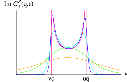
Figure 7: Spectral weight ${\rm Im}G_{+}^{R}(q,\varepsilon)$ (arbitrary units) for right movers as a function of energy for different temperatures and $u/v=1.1$. At low $T$, the SCS manifests itself in the double-peak structure, with two peaks located at $\varepsilon=vq$ and $\varepsilon=uq$. When $T$ increases ($T/vq=0,\ 0.05,\ 0.1,\ 0.5$ and $1$) the singularities are rounded off and eventually a single peak emerges.

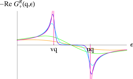
Figure 8: Real part of the right-mover Green’s function $G_{+}^{R}(q,\varepsilon)$ as a function of energy. Parameters are the same as in Fig. 7. The singularities are smoothened and the peak-dip structure broadened with increasing temperature.

To conclude, in Sec. III we have analyzed the behavior of single-particle excitations in a spinful LL at finite $T$. We have demonstrated that, because of the SCS, it is dramatically modified as compared to the spinless case. In particular, the decay length $l_{ee}$ turned out to be parametrically shorter than for spinless electrons. However, a priori it is not immediately clear to what extent the modification of the single-particle properties will affect the transport (i.e., two-particle for fermions) properties of a spinful LL. Indeed, as shown in Refs. GMPlett, ; GMP, for the spinless case, the WL dephasing length $l_{\phi}$ is parametrically longer than $l_{ee}$. Calculation of the conductivity of a disordered quantum wire in the presence of spin is a subject of the next section.

IV Weak Localization

So far we have analyzed the single-particle properties of a spinful LL at finite $T$ in the absence of disorder. Now we introduce disorder and turn to the calculation of a two-particle quantity, namely, the conductivity. At high $T$, the leading term in the conductivity is given by the Drude formula,

$$\sigma_{\rm D}=\frac{2e^{2}}{\pi}l,$$ (4.1)

with a renormalized mattis74 ; luther74 ; giam88 ; kane92 by interaction—therefore temperature dependent—mean free path $l\propto T^{\alpha_{r}}$.

We consider now a correction $\Delta\sigma$ to the Drude conductivity, associated with the quantum interference of electron waves multiple-scattered off disorder. In 1D, the leading contribution to $\Delta\sigma$ comes from a Cooperon-type scattering process which, in contrast to higher dimensionalities, involves a minimal possible number of scatterings on impurities, namely three (“three-impurity Cooperon”).GMPlett ; GMP The peculiarity of 1D in this respect is that a single-channel quantum wire is in the WL regime—not strongly localized—only if the dephasing length $l_{\phi}$ that cuts off the WL correction is shorter than the mean free path $l$. That is, the WL correction is accumulated on ballistic scales—hence the shortest possible Cooperon ladder with three impurity legs.

IV.1 General expression for Cooperon

The leading term in $\Delta\sigma$ is given by the diagramsGMPlett ; GMP in Fig. 9. These are understood as dressed by interaction-induced fluctuating gauge factors $\exp[\pm i\theta_{\mu}(x,\tau)]$ attached pairwise to the backscattering vertices, as described in Sec. II.3 and illustrated in Fig. 10 for the case of diagram (a). The sum of contributions of diagrams (b) and (c) is equal to that of diagram (a). At this level, there is no difference in the structure of the diagrams between the spinful and spinless cases—the only difference stems from the particular form of the correlators of the phases $\theta_{\mu}(x,\tau)$.

Figure 9: Diagrams giving the leading contribution to the interference correction to the conductivity. The dashed lines represent the impurity scatterings and the solid lines denote the electron Green’s functions (with the disorder effects incorporated at the self-energy level) and the dashed lines represent the impurity-induced backscattering. The diagrams are understood as “dressed” by interaction as shown in Fig. 10.

Figure 10: The same diagram as in Fig. 9a with the interaction-induced factors $\exp(\pm i\theta_{\mu})$ shown explicitly. The solid lines with arrows stand for bare Green’s functions, the crosses for the impurity vertices, and the wavy lines for the factors $\exp(\pm i\theta_{\mu})$. The space-time coordinates of the backscattering vertices are denoted by $N=(x_{N},\tau_{N})$ and ${\bar{N}}=(x_{N},{\bar{\tau}}_{N})$. Averaging over the fields $\theta_{\mu}$ couples all wavy lines with each other, cf. Fig. 3.

Averaging over the fields $\theta_{\mu}(x,\tau)$, we get for the interefernce correction at Matsubara frequency $\Omega_{m}$:

$$\Delta\sigma(i\Omega_{m}) = 2\times 2\times 2\times(ev)^{2}\times\left({v^{2}\over 2l_{0}}\right)^{3}\times{1\over\Omega_{m}}$$ (4.2)

$$\times \frac{T}{L}\int_{0}^{1/T}\!d\tau_{1}\int_{0}^{1/T}\!d\bar{\tau}_{1}\int_{0}^{1/T}\!d\tau_{2}\int_{0}^{1/T}\!d\bar{\tau}_{2}\int_{0}^{1/T}\!d\tau_{3}\int_{0}^{1/T}\!d\bar{\tau}_{3}\,\int\!dx_{1}\int\!dx_{2}\int\!dx_{3}$$

$$\times \left[g_{+}(x_{1}-x_{3},\tau_{1}-\bar{\tau}_{3})Q^{-1}(x_{1}-x_{3},\tau_{1}-\bar{\tau}_{3})\right]\,\left[g_{-}(x_{2}-x_{1},\tau_{2}-\tau_{1})Q^{-1}(x_{2}-x_{1},\tau_{2}-\tau_{1})\right]$$

$$\times \left[g_{+}(x_{3}-x_{2},\tau_{3}-\tau_{2})Q^{-1}(x_{3}-x_{2},\tau_{3}-\tau_{2})\right]\,\left[g_{-}(x_{1}-x_{3},\bar{\tau}_{1}-\tau_{3})Q^{-1}(x_{1}-x_{3},\bar{\tau}_{1}-\tau_{3})\right]$$

$$\times \left[g_{+}(x_{2}-x_{1},\bar{\tau}_{2}-\bar{\tau}_{1})Q^{-1}(x_{2}-x_{1},\bar{\tau}_{2}-\bar{\tau}_{1})\right]\,\left[g_{-}(x_{3}-x_{2},\bar{\tau}_{3}-\bar{\tau}_{2})Q^{-1}(x_{3}-x_{2},\bar{\tau}_{3}-\bar{\tau}_{2})\right]$$

$$\times Q(x_{1}-x_{3},\tau_{1}-\tau_{3})\,Q(x_{1}-x_{3},\bar{\tau}_{1}-\bar{\tau}_{3})\,Q(x_{1}-x_{2},\tau_{1}-\bar{\tau}_{2})$$

$$\times Q(x_{2}-x_{1},\tau_{2}-\bar{\tau}_{1})\,Q(x_{3}-x_{2},\tau_{3}-\bar{\tau}_{2})\,Q(x_{2}-x_{3},\tau_{2}-\bar{\tau}_{3})$$

$$\times Q^{-1}(0,\tau_{1}-\bar{\tau}_{1})\,Q^{-1}(0,\tau_{2}-\bar{\tau}_{2})\,Q^{-1}(0,\tau_{3}-\bar{\tau}_{3})$$

$$\times {\cal W}_{+}^{i}(x_{1}-x_{3},\tau_{1},\bar{\tau}_{3},\Omega_{m}){\cal W}_{-}^{f}(x_{1}-x_{3},\bar{\tau}_{1},\tau_{3},\Omega_{m})~{},$$

where $L$ is the system size, the free Green’s functions $g_{\pm}(x,\tau)$ are given by Eq. (3.1), the interaction-induced factors $Q(x,\tau)$ are defined by Eq. (2.22), and the factors ${\cal W}_{\pm}^{i,f}(x,\tau,\tau^{\prime},\Omega_{m})$ come from integration of the two Green’s functions attached to the current vertices over the external coordinates and times:

$${\cal W}_{+}^{i}(x,\tau,\tau^{\prime},\Omega_{m}) = \displaystyle{{{\rm sgn}\Omega_{m}\over|\Omega_{m}|+v/l}}\Big{\{}\left(e^{-i\Omega_{m}\tau}-e^{-i\Omega_{m}\tau^{\prime}}\right)+{v\over|\Omega_{m}|l}\left(1-e^{-|\Omega_{m}x|/v}\right)$$ (4.3)

$$\times \left[e^{-i\Omega_{m}\tau}\theta(\Omega_{m}x)-e^{-i\Omega_{m}\tau^{\prime}}\theta(-\Omega_{m}x)\right]\Big{\}},$$

$${\cal W}_{-}^{i,f}(x,\tau,\tau^{\prime},\Omega_{m}) = -{\cal W}_{+}^{i,f}(-x,\tau,\tau^{\prime},\Omega_{m}),$$

$${\cal W}_{+}^{f}(x,\tau,\tau^{\prime},\Omega_{m}) = {\cal W}_{+}^{i}(x,\tau,\tau^{\prime},-\Omega_{m}).$$ (4.4)

In Eq. (4.3), we have included vertex corrections for the current vertices, which arise from the anisotropy of impurity scattering [recall that only backscattering off impurities (2.3) is retained in the model]. The vertex corrections result in a replacement of the total scattering rate $v/2l$ by the transport scattering rate $v/l$. Note also that Eq. (4.2) is written in terms of the contribution of the Cooperon with chiralities of the current vertices as shown in Fig. 10. The numerical coefficient in Eq. (4.2) takes into account that $\Delta\sigma_{\rm WL}$ is a factor of $2\times 2\times 2=8$ larger than the contribution of the diagram in Fig 10 [one of the factors of 2 comes from the spin, another from a summation over chiralities of the current vertices and the third one from diagrams (b) and (c) in Fig. 9].

The approximation (3.4) means that the terms in the exponent of $Q(x,\tau)$ [Eqs. (2.21),(2.22), and(2.26)] that come from $B_{++}(x,\tau)$ and $B_{--}(x,\tau)$ and are proportional to $\alpha_{b}$ are neglected. As for the term that comes from $B_{+-}(x,\tau)$ and is proportional to $\alpha_{r}$, it leads to a renormalization of the impurity strength (see Ref. GMP, for details) but does not contribute to the dephasing rate to first order in $\alpha$, similarly to the spinless case. Therefore, in the calculation below we put both $\alpha_{b}$ and $\alpha_{r}$ in $Q(x,\tau)$ equal to zero, while $l_{0}$ is replaced by $l$ which is understood as the renormalized mean free path. The factor $Q(x,\tau)$ in the limit of small $\alpha$ is then written as

$$Q(x,\tau)\simeq\sqrt{{\sinh[\pi T(x/u+i\tau)]\sinh[\pi T(x/u-i\tau)]\over\sinh[\pi T(x/v+i\tau)]\sinh[\pi T(x/v-i\tau)]}}~{}.$$

(4.5)

The second term in Eq. (4.3), proportional to $1/l$, can be omitted for $l_{\phi}/l\ll 1$, so that one more approximation we make is to take the factors (4.3) in Eq. (4.2) at $x=0$:

$${\cal W}_{+}^{i}(0,\tau,\tau^{\prime},\Omega_{m})={{\rm sgn}\Omega_{m}\over|\Omega_{m}|+v/l}\left(e^{-i\Omega_{m}\tau}-e^{-i\Omega_{m}\tau^{\prime}}\right)~{}.$$ (4.6)

It is convenient to introduce new variables

$$x_{a} = x_{1}-x_{3}~{},$$

$$x_{b} = x_{3}-x_{2}~{},$$

$$x_{c} = x_{1}-x_{2}~{},$$ (4.7)

and

$$\tau_{a} = \tau_{1}-\bar{\tau}_{3}~{},$$

$$\tau_{c} = \tau_{2}-\tau_{1}~{},$$

$$\tau_{b} = \tau_{3}-\tau_{2},$$

$$\bar{\tau}_{a} = \bar{\tau}_{1}-\tau_{3}~{},$$

$$\bar{\tau}_{c} = \bar{\tau}_{2}-\bar{\tau}_{1}~{},$$

$$\bar{\tau}_{b} = \bar{\tau}_{3}-\bar{\tau}_{2}~{}.$$ (4.8)

These satisfy the constraints $x_{c}=x_{a}+x_{b}$ and $\tau_{a}+\tau_{b}+\tau_{c}+\bar{\tau}_{a}+\bar{\tau}_{b}+\bar{\tau}_{c}=0$. We thus represent Eq. (4.2) as an integral over the variables (4.7),(4.8) and insert, instead of $T/L$, in the integrand the factor

$$T\sum_{n}e^{i\varepsilon_{n}(\tau_{a}+\tau_{b}+\tau_{c}+\bar{\tau}_{a}+\bar{\tau}_{b}+\bar{\tau}_{c})}\delta(x_{c}-x_{a}-x_{b})$$ (4.9)

which contains summation over fermionic Matsubara frequencies. By extracting the vertex functions (4.3) at $x=0$, Eq. (4.2) in the limit $\alpha\ll 1$ is rewritten in the new variables as

$$\frac{\Delta\sigma}{\sigma_{\rm D}} \simeq \lim_{\Omega\to 0}\,\Big{\{}\,-\,{2\pi T\over\Omega_{m}}\,\,{v^{4}\over(|\Omega_{m}|+v/l)^{2}}\,\,\sum_{n}\int_{0}^{1/T}\!\!d\,\tau_{a}\,d\,\tau_{b}\,d\,\tau_{c}\,d\,\bar{\tau}_{a}\,d\,\bar{\tau}_{b}\,d\,\bar{\tau}_{c}\,\,\int d\,x_{a}\,d\,x_{b}\,d\,x_{c}\,$$ (4.10)

$$\times G_{+}(x_{a},\tau_{a})\,\,G_{-}(x_{a},\bar{\tau}_{a})\,\,G_{+}(x_{c},\tau_{c})\,\,G_{-}(x_{c},\bar{\tau}_{c})\,\,G_{+}(x_{b},\tau_{b})\,\,G_{-}(x_{b},\bar{\tau}_{b})\,$$

$$\times C_{+}(x_{a},\tau_{a})\,\,C_{-}(x_{a},\bar{\tau}_{a})\,\,C_{+}(x_{c},\tau_{c})\,\,C_{-}(x_{c},\bar{\tau}_{c})\,\,C_{+}(x_{b},\tau_{b})\,\,C_{-}(x_{b},\bar{\tau}_{b})\,$$

$$\times Q(x_{a},\tau_{b}+\tau_{c})\,Q(x_{a},\bar{\tau}_{b}+\bar{\tau}_{c})\,Q(x_{c},\tau_{a}+\bar{\tau}_{b})\,Q(x_{c},\bar{\tau}_{a}+\tau_{b})\,Q(x_{b},\bar{\tau}_{a}+\bar{\tau}_{c})\,Q(x_{b},\tau_{a}+\tau_{c})\,$$

$$\times \exp[\,i(\Omega_{m}+\varepsilon_{n})\,(\,\tau_{a}+\tau_{b}+\tau_{c}\,)-i\varepsilon_{n}\,(\,\bar{\tau}_{a}+\bar{\tau}_{b}+\bar{\tau}_{c}\,)\,]\,\,\delta\,(x_{a}+x_{b}-x_{c})\,\Big{\}}_{i\Omega_{m}\to\Omega+i0},$$

where $G_{\pm}(x,\tau)$ is given by Eq. (3.4), $Q(x,\tau)$ by Eq. (4.5), and we introduce

$$C_{\pm}(x,\tau)=\sqrt{{\sinh[\pi T(x/v\mp i\tau)]\over\sinh[\pi T(x/u\mp i\tau)]}}~{},$$ (4.11)

such that $g_{\pm}Q^{-1}\simeq G_{\pm}C_{\pm}$. When deriving Eq. (4.10) we have used the approximation (4.6)

$${\cal W}_{+}^{i}(0,\tau_{1},\bar{\tau}_{3},\Omega_{m}){\cal W}_{-}^{f}(0,\bar{\tau}_{1},\tau_{3},\Omega_{m}) \to \displaystyle{{1\over(|\Omega_{m}|+v/l)^{2}}}\,\Big{[}-e^{i\Omega_{m}(\tau_{1}-\bar{\tau}_{1})}-e^{i\Omega_{m}(\bar{\tau}_{3}-\tau_{3})}$$ (4.12)

$$+ e^{i\Omega_{m}(\tau_{1}-\tau_{3})}+e^{i\Omega_{m}(\bar{\tau}_{3}-\bar{\tau}_{1})}\Big{]}\to-\displaystyle{{2\,e^{i\Omega_{m}(\bar{\tau}_{3}-\tau_{3})}\over(|\Omega_{m}|+v/l)^{2}}}.$$

The “diagonal” terms $\exp[i\Omega_{m}(\bar{\tau}_{1}-\tau_{1})]$ and $\exp[i\Omega_{m}(\tau_{3}-\bar{\tau}_{3})]$ yield identical contributions [which is accounted for by the factor of 2 in Eq. (4.10)]. The cross-terms are neglected, since, after the integration over times (see Secs. IV.2 and V below), they produce the products of Green’s functions in the $(x,\varepsilon)$ representation of the type

$$G^{r(a)}_{+}(x,\varepsilon_{n})G^{r(a)}_{-}(x,\varepsilon_{k})=0$$ (4.13)

[see Eq. (3.15)]. This corresponds to retaining only those Cooperon diagrams that contain an equal number of the retarded and advanced Green’s functions, even with e-e interaction included.

We are thus left with the functions $G_{\pm}(x,\tau)$, $Q(x,\tau)$, and $C_{\pm}(x,\tau)$ that are all given by various combinations of square-root factors $\sqrt{\sinh[\pi T(x/u\pm i\tau)]}$ and $\sqrt{\sinh[\pi T(x/v\pm i\tau)]}$. Note that $G_{\pm}(x,\tau)$ and $C_{\pm}(x,\tau)$ enter Eq. (4.10) only in the combination $G_{\pm}C_{\pm}$ with the same arguments. Equation (4.10) will be analyzed in the next two subsections.

IV.2 Regular impurity configurations: Weak localization

In Eq. (4.10), we transform the integration contours for each of the time variables similarly to Fig. 4. As a result, we obtain integrals along square-root branch cuts in the vertical direction, each of which connects two points whose coordinates can be written as $\tau+ix/u$ and $\tau+ix/v$ with different $\tau$ and $x$. For example, let us assume, here and throughout the paper below, that in Eq. (4.10) all

$$x_{a},x_{b},x_{c}>0$$ (4.14)

(the region of integration $x_{a}<0$ and $x_{b},x_{c}>0$ gives the same contribution to $\Delta\sigma_{\rm WL}$). Then, starting with the integration over $\tau_{a}$ and closing the contour upwards, we represent the integral along the real axis of $\tau_{a}$ as a sum of three integrals around vertical cuts: between $ix_{a}/u$ and $ix_{a}/v$, between $-\bar{\tau}_{b}+ix_{c}/u$ and $-\bar{\tau}_{b}+ix_{c}/v$, and between $-\bar{\tau}_{c}+ix_{b}/u$ and $-\bar{\tau}_{c}+ix_{b}/v$. The first cut comes from the Green’s function $G_{+}(x_{a},\tau_{a})$, whereas the last two from the factors $Q(x_{b},\tau_{a}+\tau_{c})$ and $Q(x_{c},\tau_{a}+\bar{\tau}_{b})$, respectively. Since $G_{+}(x,\tau)$ as a function of $x$ for a given $\tau$ falls of on the scale of $l_{T}$, while $Q(x,\tau)$ on the scale of $l_{ee}$, one sees that in the limit of small $\alpha$ the main contribution to $\Delta\sigma_{\rm WL}$ comes from the branch cuts that are associated with the Green’s functions. The cuts related to the factors $Q(x,\tau)$ can be neglected.

The selection of singularities at $\alpha\ll 1$ is closely analogous to that in the spinless case, see Appendix F of Ref. GMP, . For spinless electrons, the main contribution to $\Delta\sigma_{\rm WL}$ stems from singularities (“nearly poles” for weak interaction) of the single-particle Green’s functions at the classical trajectory of an electron moving with the velocity $u$. Other close-to-pole singularities (those in the factors $Q$ and $C$), which are related to “nonclassical trajectories”, yield subleading corrections small in the parameter $l_{T}/l_{\phi}\ll 1$. The spinful problem is very much similar in this respect. The main difference is that the dominant singularities are now pairs of close square-root branching points rather than the poles. The transformation of the poles into the branch cuts, induced by the SCS, can be viewed as a “smearing” of the classical trajectories: all velocities between $v$ and $u$ become accessible.

Let us first consider the contribution to Eq. (4.10) from typical impurity configuration for which the characteristic scale of

$$x_{a}\sim x_{b}\sim x_{c}$$ (4.15)

is of the order of $l_{\phi}\gg l_{T}$. We can then expand all $\sinh$’s in the $C$ and $Q$ factors as

$$\sinh(\pi Ty)\simeq{1\over 2}e^{\pi T|y|}\,{\rm sgn}\,y~{},\qquad|y|\gg 1~{}.$$ (4.16)

It is immediately seen that using Eq. (4.16) reduces the product of six $C$ factors to a simple exponential:

$${\cal C}\simeq\exp(2x_{c}/l_{ee})~{}.$$ (4.17)

Similarly, the product of six $Q$ factors

$${\cal Q} = Q\left[x_{a},i\left(t_{c}+t_{b}+{2x_{b}+x_{a}\over u}\right)\right]Q\left[x_{a},i\left(\bar{t}_{c}+\bar{t}_{b}+{2x_{b}+x_{a}\over u}\right)\right]Q\left[x_{c},i\left(t_{a}-\bar{t}_{b}+{x_{a}-x_{b}\over u}\right)\right]$$ (4.18)

$$\times Q\left[x_{c},i\left(t_{b}-\bar{t}_{a}+{x_{b}-x_{a}\over u}\right)\right]Q\left[x_{b},i\left(t_{a}+t_{c}+{2x_{a}+x_{b}\over u}\right)\right]Q\left[x_{b},i\left(\bar{t}_{a}+\bar{t}_{c}+{2x_{a}+x_{b}\over u}\right)\right]$$

is represented as

$${\cal Q}\simeq\exp(\pi Tq/2)~{},$$ (4.19)

where

$$q = |2x_{b}/u+t_{c}+t_{b}|-|2x_{b}/u+t_{c}+t_{b}-2x_{a}/u_{-}|+|2x_{c}/u+t_{c}+t_{b}|-|2x_{c}/u+t_{c}+t_{b}+2x_{a}/u_{-}|$$ (4.20)

$$+ |2x_{b}/u+\bar{t}_{c}+\bar{t}_{b}|-|2x_{b}/u+\bar{t}_{c}+\bar{t}_{b}-2x_{a}/u_{-}|+|2x_{c}/u+\bar{t}_{c}+\bar{t}_{b}|-|2x_{c}/u+\bar{t}_{c}+\bar{t}_{b}+2x_{a}/u_{-}|$$

$$+ |2x_{b}/u-t_{a}+\bar{t}_{b}|-|2x_{b}/u-t_{a}+\bar{t}_{b}+2x_{c}/u_{-}|+|2x_{a}/u+t_{a}-\bar{t}_{b}|-|2x_{a}/u+t_{a}-\bar{t}_{b}+2x_{c}/u_{-}|$$

$$+ |2x_{a}/u+\bar{t}_{a}-t_{b}|-|2x_{a}/u+\bar{t}_{a}-t_{b}+2x_{c}/u_{-}|+|2x_{b}/u-\bar{t}_{a}+t_{b}|-|2x_{b}/u-\bar{t}_{a}+t_{b}+2x_{c}/u_{-}|$$

$$+ |2x_{a}/u+t_{a}+t_{c}|-|2x_{a}/u+t_{a}+t_{c}-2x_{b}/u_{-}|+|2x_{c}/u+t_{a}+t_{c}|-|2x_{c}/u+t_{a}+t_{c}+2x_{b}/u_{-}|$$

$$+ |2x_{a}/u+\bar{t}_{a}+\bar{t}_{c}|-|2x_{a}/u+\bar{t}_{a}+\bar{t}_{c}-2x_{b}/u_{-}|+|2x_{c}/u+\bar{t}_{a}+\bar{t}_{c}|-|2x_{c}/u+\bar{t}_{a}+\bar{t}_{c}+2x_{b}/u_{-}|~{}.$$

In Eqs. (4.18) and (4.20) we have shifted the time variables according to

$$i\tau_{j} = -t_{j}-x_{j}/u,$$

$$i\bar{\tau}_{j} = \bar{t}_{j}+x_{j}/u,$$ (4.21)

with $j=a,b,c$. The shifted variables $t_{j}$ and $\bar{t}_{j}$ in Eq. (4.21) are real on the branch cuts corresponding to the Green’s functions in Eq. (4.10) and change along these cuts from 0 to $2x_{j}/u_{-}\sim\alpha x_{j}/u$, where $u_{-}$ is given by Eq. (3.11). Inspecting Eq. (4.20), we observe that for $x_{a}>2x_{c}u/u_{-}$ (or similarly for $x_{b}$) all the moduli can in fact be omitted on the Green’s function branch cuts, which yields

$${\cal Q}\simeq\exp(-4\pi Tx_{c}/u_{-})=\exp(-2x_{c}/l_{ee})$$ (4.22)

(the opposite case $x_{a,b}<2\alpha x_{c}$ is addressed in Sec. V). As a result, the factors $\cal C$ and $\cal Q$ compensate each other:

$${\cal QC}\simeq 1~{}.$$ (4.23)

The integrand of Eq. (4.10) thus reduces to a product of the single-particle Green’s functions in the $(x,\varepsilon)$ representation [Eqs. (3.15), (3.17)]:

$$\frac{\Delta\sigma_{\rm WL}}{\sigma_{\rm D}} = \lim_{\Omega\to 0}\Big{\{}\,-\,{2\pi T\over\Omega_{m}}\,\,{v^{4}\over(|\Omega_{m}|+v/l)^{2}}\,\,\sum_{n}\,\int_{0}^{\infty}dx_{a}\,dx_{b}\,dx_{c}\,\delta\,(x_{a}+x_{b}-x_{c})$$

$$\times G_{+}^{r}(x_{a},i\varepsilon_{n}+i\Omega_{m})G_{+}^{r}(x_{c},i\varepsilon_{n}+i\Omega_{m})G_{+}^{r}(x_{b},i\varepsilon_{n}+i\Omega_{m})G_{-}^{a}(x_{a},i\varepsilon_{n})G_{-}^{a}(x_{c},i\varepsilon_{n})G_{-}^{a}(x_{b},i\varepsilon_{n})\Big{\}}_{i\Omega_{m}\to\Omega+i0}~{},$$

where we have taken into account that only terms with $\varepsilon_{n}<0,\ \varepsilon_{n}+\Omega_{m}>0$ survive, in view of Eq. (4.13), which follows from Eq. (3.15). Performing the analytical continuation to real frequencies $\Omega_{m}\to\Omega+i0$, we get in the dc limit $\Omega\to 0$:

$${\Delta\sigma_{\rm WL}\over\sigma_{\rm D}}=-A_{\rm WL}\Big{(}{l_{ee}\over l}\Big{)}^{2}\ ,$$ (4.25)

where the numerical factor $A_{\rm WL}$ is defined by

$$A_{\rm WL}=\pi\int_{-\infty}^{\infty}\,{dz\over{\rm cosh}^{2}\pi z}\,\int_{0}^{\infty}dx\,\int_{0}^{\infty}dy\,{\cal R}(x,z)\,{\cal R}(y,z)\,{\cal R}(x+y+xy,z),$$ (4.26)

with

$${\cal R}(x,z)=\,_{2}{\rm F}_{1}\left(\,1/2+iz,\,1/2,\,1;\,-x\,\right)\,_{2}{\rm F}_{1}\left(\,1/2-iz,\,1/2,\,1;\,-x\,\right).$$ (4.27)

We have estimated $A_{\rm WL}\simeq 0.13$ by taking the integral (4.26) numerically.

The small factor $(l_{ee}/l)^{2}$ in Eq. (4.25) is due to the exponential decay $\exp(-2x_{c}/l_{ee})$ of the product of six Green’s functions in the integrand of Eq. (LABEL:58-1) on the scale of $l_{ee}$. One sees that the dephasing factor that suppresses the interference term in the conductivity behaves as $\exp(-L_{C}/l_{\phi})$, where $L_{C}=x_{a}+x_{b}+x_{c}=2x_{c}$ is the total length of the Cooperon loop and the WL dephasing length $l_{\phi}$ reads

$$l_{\phi}=l_{ee}~{}.$$ (4.28)

Schematically, Eq. (LABEL:58-1) can be estimated as

$${\Delta\sigma_{\rm WL}\over\sigma_{\rm D}}\sim - \int_{0}^{\infty}\frac{dx_{a}}{l}\exp(-2x_{a}/l_{ee})$$

$$\times \int_{0}^{\infty}\frac{dx_{b}}{l}\exp(-2x_{b}/l_{ee})\sim-\Big{(}{l_{ee}\over l}\Big{)}^{2}~{},$$

so that for typical realizations of disorder with $x_{a}\sim x_{b}\sim x_{c}$ each of the distances is of the order of $l_{ee}$, see Fig. 11a. For comparison, in the spinless case,GMPlett ; GMP the relevant distances obey $x_{a}x_{b}\sim ll_{ee}$, which yields

$${\Delta\sigma_{\rm WL}^{sl}\over\sigma_{\rm D}} \sim -\int_{0}^{l}\frac{dx_{a}}{l}\int_{0}^{l}\frac{dx_{b}}{l}\,\exp(-x_{a}x_{b}/ll_{ee})$$

$$\sim -{l_{ee}\over l}\,\ln{l\over l_{ee}}\sim-\left({l_{\phi}\over l}\right)^{2}\,\ln{l\over l_{\phi}}~{}.$$

It follows that $l_{\phi}$ for spinful electrons is much shorter than the dephasing length for spinless electrons (recall that for the latter, $l_{\phi}$ divergesGMPlett ; GMP in the limit of vanishing disorder). In fact, in the spinful case $l_{\phi}$ is equal to the single-particle (electron) decay length $l_{ee}$, in contrast to the spinless case, where $l_{\phi}\gg l_{ee}$.

V Anomalous Impurity Configurations: Memory Effects

The WL contribution to the conductivity, calculated in the preceding section, is associated with scattering on compact three-impurity configurations which are “regular” in the sense that the characteristic distances between all three impurities are the same. Below, we will see that “anomalous” (strongly asymmetric) configurations in which two of the impurities are anomalously close to each other, i.e., $x_{a}\ll x_{b}$ or $x_{b}\ll x_{a}$ (see Fig. 11b), give rise to a conductivity correction which is larger than $\Delta\sigma_{\rm WL}$ if $T$ is sufficiently high. As mentioned already in Sec. I, the relevance of the asymmetric configurations is related to the classical MEzero-omega in electron kinetics, in contrast to the quantum interference of scattered waves that yields $\Delta\sigma_{\rm WL}$.

Figure 11: Three-impurity configurations that give the main contribution to the (a) quantum (WL) and (b) classical (ME) corrections to the conductivity. The characteristic distances between the impurities are shown.

V.1 Qualitative consideration: Identifying scales and parameters

To demonstrate the peculiarity of the asymmetric impurity configurations, it is instructive to consider first the limit of two scattering events occurring at the same point, by setting

$$x_{1}=x_{3}$$ (5.1)

in Eq. (4.2). As discussed at the beginning of Sec. IVB, for typical impurity configurations (4.15) the main contribution to the correction (4.2) comes from “smeared” classical trajectories, meaning that all trajectories with velocities between $v$ and $u$ contribute to $\Delta\sigma_{\rm WL}$. The case (5.1) is, however, special in that only one velocity remains and that is the velocity of noninteracting electrons $v$. Indeed, at $x_{1}=x_{3}$ the four $Q$ factors that depend on $x_{1}-x_{3}$ drop out of the integration over times—since $Q(0,\tau)$ [Eq. (4.5)] does not depend on $\tau$. After this, the integrals in Eq. (4.2) over $\tau_{1}$ and $\bar{\tau}_{1}$ are dominated by the poles of the noninteracting Green’s functions $g_{+}(0,\tau_{1}-\bar{\tau}_{3})$ and $g_{-}(0,\bar{\tau}_{1}-\tau_{3})$, which yields

$$\tau_{1}={\bar{\tau}}_{3},\quad{\bar{\tau}}_{1}=\tau_{3},$$ (5.2)

and then all the remaining factors $Q$ compensate each other. We thus end up with a product of six bare Green’s functions $g_{\pm}$ multiplied by the factors ${\cal W}_{\pm}$, which constitutes the noninteracting limit of the problem.footnon

In fact, the compensation of the dephasing factors is evident even before the averaging over the fluctuating fields $\theta_{\pm}(x,\tau)$ (Fig. 10). Indeed, the factors $\exp\{\pm i[\theta_{+}(x,\tau)-\theta_{-}(x,\tau)]\}$, dressing two impurity vertices, cancel each other when taken at the same space-time point [Eqs. (5.1) and (5.2)]. As a result, the third impurity located at $x_{2}$ becomes decoupled with respect to e-e interaction from the two-impurity complex at $x_{1}=x_{3}$.

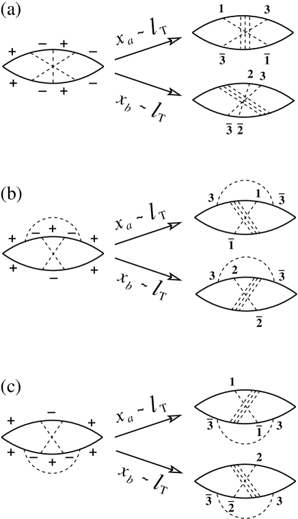
Figure 12: Each diagram for $\Delta\sigma$ in Fig. 9 has two ME contributions, coming from $x_{a}\sim l_{T}$ ($\bar{3}\to 1$, $\bar{1}\to 3$) and $x_{b}\sim l_{T}$ ($2\to 3$, $\bar{2}\to\bar{3}$). The remote-impurity line should be replaced by the full diffuson ladder.

In the cyclic variables (4.7), Eq. (5.1) means $x_{a}=0$. Since interaction completely drops out of the problem at $x_{a}=0$, the integration over the remaining spatial coordinate $x_{b}=x_{c}$ in Eq. (4.10) is not cut off by dephasing, in contrast to the regular impurity configurations, for which it is restricted to $x_{c}\lesssim l_{ee}\ll l$. In this situation, we have to take into account a disorder-induced damping of the single-particle Green’s functions $g_{\pm}(x,\tau)$, which results in an additional factor $\exp(-|x|/4l)$ attached to each $g_{\pm}(x,\tau)$. On the Cooperon loop, these combine to give the overall factor $\exp(-x_{c}/l)$ in the integrand of Eq. (4.2), so that $x_{b}=x_{c}$ is then limited by the mean free path, see Fig. 11b.

Since at $x_{a}=0$ the characteristic distance to the remote third impurity in the three-impurity Cooperon diagram happens to be in the crossover region between the ballistic and diffusive motion, we should extend the single scattering on the third impurity to an infinite sequence of scatterings on other impurities,footnote-ladder i.e., to a diffuson ladder, as shown in Fig. 12. One sees that the diagram takes the form characteristic of a quasiclassical ME:zero-omega an electron is scattered at $x_{1}\simeq x_{3}$, then moves around diffusively, and returns to $x_{1}\simeq x_{3}$ where it is scattered once again. Clearly, this is a non-Markovian process which is beyond the conventional Boltzmann description. However, the non-Boltzmann type of kinetics associated with the return processes is classical in origin: as discussed above, when the points $x_{1}$ and $x_{3}$ are sufficiently close to each other, dephasing becomes irrelevant. We will first analyze the simplest three-impurity diagram at finite but small $x_{a}$ and include the diffusive returns (which will only renormalize the numerical prefactor) later in the end of this section.

It is instructive to begin with a semi-quantitative analysis which will give correctly the parametric dependence of the result but not the numerical coefficient. To this end, we replace all hyperbolic sines in both the Green’s functions $G_{\pm}$ and the $Q$ and $C_{\pm}$ factors in Eq. (4.10) by their exponential asymptotics, Eq. (4.16). This approximation is parametrically correct, since all integrals in Eq. (4.16) are determined by the regions of integration in which the arguments of the hyperbolic sines are of the order of or larger than 1. Within the “exponential” approximation, the product ${\cal C}$ of six factors $C_{\pm}$ is given by Eq. (4.17), while the product ${\cal G}$ of six Green’s functions in Eq. (4.16) becomes

$${\cal G}\propto\exp(-2x_{c}/l_{ee})~{},$$ (5.3)

so that the exponential factors in $\cal G$ and $\cal C$ cancel each other, similarly to the regular impurity configurations in Sec. IV.2. What is different, however, is that when calculating the factor ${\cal Q}$ [Eqs. (4.18)–(4.20)] one can no longer omit the moduli in Eq. (4.20) if

$$x_{a}<2\alpha x_{c}$$ (5.4)

[or $x_{b}<2\alpha x_{c}$—we will proceed with the estimate for the case of Eq. (5.4)]. For the strongly asymmetric configurations (5.4), Eq. (4.20) is rewritten as

$$q \simeq -8x_{c}/u_{-}+\big{|}2x_{a}/u-t_{b}\big{|}-\big{|}2x_{a}/u-t_{b}+2x_{c}/u_{-}\big{|}+\big{|}2x_{a}/u-\bar{t}_{b}\big{|}-\big{|}2x_{a}/u-\bar{t}_{b}+2x_{c}/u_{-}\big{|}$$ (5.5)

$$+\big{|}2x_{a}/u+t_{c}\big{|}-\big{|}2x_{a}/u+t_{c}-2x_{c}/u_{-}\big{|}+\big{|}2x_{a}/u+\bar{t}_{c}\big{|}-\big{|}2x_{a}/u+\bar{t}_{c}-2x_{c}/u_{-}\big{|}~{},$$

where we have neglected terms of second order in $\alpha$. In particular, the integration over $t_{a}$ and $\bar{t}_{a}$ goes along very short branch cuts of length $\propto\alpha x_{a}\sim\alpha^{2}x_{c}$. To our accuracy, the cuts reduce to poles. For this reason, we have set $t_{a}=\bar{t}_{a}=0$ in Eq. (5.5).

The integrals over remaining time variables in Eq. (4.10) decouple from each other and can be easily calculated (note that the integrals over $t_{b}$ and $t_{c}$ are identical—in the dc limit—to those over $\bar{t}_{b}$ and $\bar{t}_{c}$, respectively). Let us denote $\Delta\sigma_{\rm asym}$ the contribution to the conductivity that comes from the strongly asymmetric impurity configurations with $|x_{a,b}|<2\alpha x_{c}$. Carrying out the analytical continuation for both fermionic and bosonic frequencies and taking the dc limit, we get, within the exponential approximation:

$$\frac{\Delta\sigma_{\rm asym}}{\sigma_{\rm D}} \sim -{1\over l^{2}}\int_{0}^{\infty}\!{d\varepsilon\,dx_{a}\,dx_{c}\over T\cosh^{2}(\varepsilon/2T)}\exp\left(-{x_{c}\over l}\right)\exp\left(-{2x_{c}\over l_{ee}}\right)$$ (5.6)

$$\times \left[\,\theta(x_{a}-\alpha x_{c})\theta(2\alpha x_{c}-x_{a})\,\Big{|}f_{1}\left({x_{a}\over 2l_{T}},{x_{c}\over 2l_{ee}},{\varepsilon\over\pi T}\right)\Big{|}^{4}\right.$$

$$+ \left.\theta(\alpha x_{c}-x_{a})\,\Big{|}f_{2}\left({x_{a}\over 2l_{T}},{x_{c}\over 2l_{ee}},{\varepsilon\over\pi T}\right)\Big{|}^{2}\,\Big{|}f_{3}\left({x_{a}\over 2l_{T}},{x_{c}\over 2l_{ee}}~{},{\varepsilon\over\pi T}\right)\Big{|}^{2}\,\right]~{},$$

where the functions $f_{1,2,3}$ are defined as follows

$$f_{1}(x,y,z) = {\exp(izy)-1\over iz},$$

$$f_{2}(x,y,z) = \exp[iz(y-x)]{\exp(izx)-1\over iz}-i\exp(x-y){\exp[(iz+1)(y-x)]-1\over(iz+1)},$$

$$f_{3}(x,y,z) = {\exp(izx)-1\over iz}+i\exp(-x){\exp[(iz+1)y]-\exp[(iz+1)x]\over(iz+1)}~{}.$$ (5.7)

In Eq. (5.6), the $\theta$-functions split the domain of integration over $x_{a}$ into two, $\alpha x_{c}<x_{a}<2\alpha x_{c}$ and

$$0<x_{a}<\alpha x_{c}~{}.$$ (5.8)

In the first interval of $x_{a}$, the integration over $x_{c}$ is limited by the factor $\exp(-2x_{c}/l_{ee})$ in the first line of Eq. (5.6), which yields a contribution to $\Delta\sigma_{\rm asym}/\sigma_{\rm D}$ of the order of $-l_{ee}l_{T}/l^{2}$. This is much smaller than the contribution of the regular impurity configurations [Eq. (4.22)] and can be neglected. However, the situation is qualitatively different for the interval (5.8). Indeed, for $1,x\ll y$, the functions $|f_{2}(x,y,z)|^{2}$ and $|f_{3}(x,y,z)|^{2}$ take the form

$$|f_{2}(x,y,z)|^{2} \simeq \Big{|}{\exp(izx)-1\over z}+{1\over 1+iz}\Big{|}^{2}~{},$$ (5.9)

$$|f_{3}(x,y,z)|^{2} \simeq {\exp[2(y-x)]\over(z^{2}+1)}~{}.$$ (5.10)

As a result, the factor $\exp(-2x_{c}/l_{ee})$ from the first line of Eq. (5.6) is canceled by the factor $\exp(2y)$ from Eq. (5.10). The remaining integral over $x_{c}$ is no longer restricted to $x_{c}\lesssim l_{ee}$ but rather extends to $x_{c}\sim l$, in agreement with our qualitative consideration of the ME effect for $x_{a}=0$ at the beginning of this section. The ME contribution $\Delta\sigma_{\rm ME}$ to the conductivity thus arises from the impurity configurations obeying Eq. (5.8) and is given by the second term in Eq. (5.6). It can be estimated as

$${\Delta\sigma_{\rm ME}\over\sigma_{\rm D}}\sim-\int_{0}^{\infty}\!{dx_{c}\over l}\exp\left(-{x_{c}\over l}\right)\int_{0}^{\alpha x_{c}}\!{dx_{a}\over l}\exp\left(-{2x_{a}\over l_{T}}\right)\sim-{l_{T}\over l}$$ (5.11)

and becomes much larger than the WL contribution [Eq. (4.22)] if $T$ is sufficiently high, namely if

$$T\gg v/\alpha^{2}l~{}.$$ (5.12)

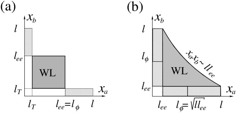
Figure 13: Domains of the distances $x_{a},x_{b}$ that govern the WL (gray-shaded area) and ME (dashed area) contributions to the conductivity for the spinful (a) and spinless (b) models.

The characteristic regions of $x_{a},x_{b}$ that control the quantum (WL) and classical (ME) corrections to the conductivity are shown in Fig. 13a. For comparison, an analogous plot for the spinless problem is presented in Fig. 13b. One sees that in the spinful case the “quantum” and “classical” domains are parametrically separated from each other. As a result, their areas $l_{ee}^{2}\propto T^{-2}$ and $ll_{T}\propto T^{-1}$, respectively, can “compete” with each other. On the contrary, in the spinless case, the ME strips of area $\sim ll_{ee}$ are directly adjacent to the WL domain, whose area $\sim ll_{ee}\ln(l/l_{ee})$ is (logarithmically) larger. It follows that for spinless electrons the ME correction $\Delta\sigma^{sl}_{\rm ME}$ gives only a subleading contribution as compared to the WL correction $\Delta\sigma^{sl}_{\rm WL}$ [Eq. (IV.2)]:

$$\left|{\Delta\sigma^{sl}_{\rm ME}\over\sigma_{\rm D}}\right|\sim{l_{ee}\over l}\ll\left|{\Delta\sigma^{sl}_{\rm WL}\over\sigma_{\rm D}}\right|\sim{l_{ee}\over l}\ln\left(\frac{l}{l_{ee}}\right)$$ (5.13)

[recall that $l_{\phi}\sim(ll_{ee})^{1/2}$ and $l_{ee}\sim\alpha^{-2}l_{T}$ for spinless electrons].

V.2 Rigorous calculation of $\Delta\sigma_{\rm ME}$

In the preceding subsection, we have adopted the “exponential approximation” by replacing all the hyperbolic sines in the correlation functions by their asymptotics (4.16). This allowed us to identify the relevant scales and obtain the parametric dependence of the result. Here, we calculating the integrals over the temporal variables $t_{b}$, ${\bar{t}}_{b}$, $t_{c}$, and ${\bar{t}}_{c}$ more accurately and find the numerical prefactor in Eq. (5.11). The estimate in Sec. V.1 teaches us that the dominant contribution to $\Delta\sigma_{\rm ME}$ comes from $x_{a}\sim l_{T}$ and $x_{b}\simeq x_{c}\sim l$, while the integrals over $t_{b,c}$ and ${\bar{t}}_{b,c}$ are determined by the upper limit of integration, i.e., by the time scale $\alpha x_{c}/v\sim\alpha l/v$. In the WL regime, this time scale is much larger than $1/T$.

Similarly to the case of regular impurity configurations, we observe that the product of all the $C$ factors can always be approximated by Eq. (4.17), whereas the hyperbolic sines should be retained in the Green’s functions $G_{\pm}$. As for the factors $Q$, in contrast to the regular configurations, not all of them can be replaced by their asymptotics. Specifically, those hyperbolic sines in the $Q$ factors that correspond to the moduli in Eq. (5.5) (i.e., all terms in $q$ except for the first one) should retain their form and not be replaced by the exponentials. Importantly, within this “partially exponential” approximation, all integrals over times are still decoupled. Thus, we replace the exponential factor depending on $t_{c}$ in Sec. V.1 according to

$$\Big{[}\,\theta\big{(}x_{a}/l_{T}+\pi Tt_{c}-x_{c}/l_{ee}\big{)}-i\theta\big{(}-x_{a}/l_{T}-\pi Tt_{c}+x_{c}/l_{ee}\big{)}\,\Big{]}$$

$$\times\,\,\exp\left[{1\over 2}\left(-x_{c}/l_{ee}+|x_{a}/l_{T}+\pi Tt_{c}|-|x_{a}/l_{T}+\pi Tt_{c}-x_{c}/l_{ee}|\right)-|\varepsilon_{n}+\Omega_{m}|\,t_{c}\right]$$

$$\rightarrow{2\exp(-|\varepsilon_{n}+\Omega_{m}|\,t_{c})\over\sinh^{1/2}(\pi Tt_{c})\sinh^{1/2}(x_{c}/l_{ee}-\pi Tt_{c})}\,{\sinh^{1/2}(x_{a}/l_{T}+\pi Tt_{c})\over\sinh^{1/2}(x_{a}/l_{T}+\pi Tt_{c}-x_{c}/l_{ee})}$$

$$\rightarrow{2\exp(x_{a}/2l_{T})\exp(-|\varepsilon_{n}+\Omega_{m}|\,t_{c})\over\sinh^{1/2}(x_{c}/l_{ee}-\pi Tt_{c})\sinh^{1/2}(x_{a}/l_{T}+\pi Tt_{c}-x_{c}/l_{ee})}$$ (5.14)

and make a similar replacement for ${\bar{t}}_{c}$ (with $\varepsilon_{n}+\Omega_{m}\to\varepsilon_{n}$). The factors depending on $t_{b}$ are modified as follows:

$$i\,\exp\left[{1\over 2}\left(-x_{c}/l_{ee}+|x_{a}/l_{T}-\pi Tt_{b}|-|x_{a}/l_{T}-\pi Tt_{b}+x_{c}/l_{ee}|\right)-|\varepsilon_{n}+\Omega_{m}|\,t_{b}\right]$$

$$\rightarrow{2\exp\left(-|\varepsilon_{n}+\Omega_{m}|\,t_{b}\right)\over\sinh^{1/2}(\pi Tt_{b})\sinh^{1/2}(x_{c}/l_{ee}-\pi Tt_{b})}\,{\sinh^{1/2}(x_{a}/l_{T}-\pi Tt_{b})\over\sinh^{1/2}(x_{a}/l_{T}-\pi Tt_{b}+x_{c}/l_{ee})}$$

$$\rightarrow{2\exp\left(-x_{a}/2l_{T}\right)\exp\left(-|\varepsilon_{n}+\Omega_{m}|\,t_{b}\right)\over\sinh^{1/2}(x_{c}/l_{ee}-\pi Tt_{b})\sinh^{1/2}(x_{a}/l_{T}-\pi Tt_{b}+x_{c}/l_{ee})},$$ (5.15)

the integral over ${\bar{t}}_{b}$ again differs only in that $\varepsilon_{n}+\Omega_{m}$ changes to $\varepsilon_{n}$. Using Eqs. (5.14) and (5.15), we get

$${\Delta\sigma_{\rm ME}\over\sigma_{\rm D}}=-A_{\rm ME}\,{l_{T}\over l}~{},$$ (5.16)

where $A_{\rm ME}$ is given by the dimensionless integral (check the first arguments of ${\rm F}$)

$$A_{\rm ME} = \pi\int_{-\infty}^{\infty}\!{dz\over\cosh^{2}\pi z}\int_{0}^{\infty}\!dx\,\,\big{|}{\cal M}(z,x)\big{|}^{2}\,\big{|}{\cal M}(z,-x)\big{|}^{2}~{}.$$

The function ${\cal M}(z,x)$ in Eq. (LABEL:108) is defined by

$${\cal M}(z,x)={1\over 2\pi}\,\int_{0}^{\infty}\!\!dy\,{\exp(2izy)\over\sinh^{1/2}(y)\sinh^{1/2}(y+x)}~{}.$$ (5.18)

We have estimated $A_{\rm ME}$ numerically as $A_{\rm ME}\simeq 0.2$.

Finally, let us discuss the overall combinatorial factor in $\Delta\sigma_{\rm ME}$ (which is already included in $A_{\rm ME}$). Firstly, similarly to the WL correction, the contribution of diagram (a) in Fig. 12 should be multiplied by a factor of $2\times 2\times 2=8$ due to (i) two possible chiralities of the current vertices; (ii) diagrams (b) and (c) in Fig. 12; and (iii) two possible anomalous configurations for each diagram: $x_{a}\sim l_{T}\ll x_{b}$ and $x_{b}\sim l_{T}\ll x_{a}$. Secondly, as mentioned above, not only the return after one single backscattering but rather the entire diffuson ladder contributes to $\Delta\sigma_{\rm ME}$ [Fig. 12]. The insertion of the diffuson into the three-impurity diagram effectively generates an additional velocity-vertex correction, which yields a factor of 1/2 (the ratio of the transport and total scattering times for the backscattering impurities).

VI Path-integral method

So far, we have been treating the conductivity correction within the formalism of Matsubara functional bosonization. This powerful method treats on an equal footing GMP the real inelastic scattering processes responsible for dephasing and the virtual transitions responsible for the renormalization effects. An alternative approach, formulated for the spinless case in Refs. GMPlett, and GMP, , consists of two steps. Firstly, disorder is renormalized by virtual processes with characteristic energy transfer larger than $T$. What is obtained after the renormalization is an effective “low-energy” theory which is free of ultraviolet singularities characteristic of a LL. The low-energy theory is treated by means of a path-integral approach, analogous to the one developed in Ref. AAK, for higher-dimensional systems. This method is particularly convenient for an analysis of inelastic scattering (dephasing) in problems with a nontrivial infrared behavior. In Ref. GMP, , the WL correction to the conductivity was calculated both within the path-integral and the functional-bosonization schemes, with identical results. The path-integral calculation also allows one to “visualize” the origin of the dephasing processes in terms of quasiclassical trajectories.

In this section, we present a path-integral analysis of the conductivity correction in the spinful problem. It turns out that the situation here is more intricate than in the spinless case, for two reasons: (i) the characteristic energy transfer in the path-integral calculation is of the order of $T$ (while it was much smaller than $T$ for spinless electrons); (ii) because of the SCS, the velocity of the quasiclassical trajectories is not uniquely defined: the whole interval of velocities between $v$ and $u$ contributes to $\Delta\sigma_{\rm WL}$, see Sec. III. As a result, we will only be able to reproduce the parametrical dependence of the conductivity correction but not the numerical prefactor. Nevertheless, this analysis is useful, since it yields a physically transparent picture of the quantum interference and dephasing in the spin-charge separated system.

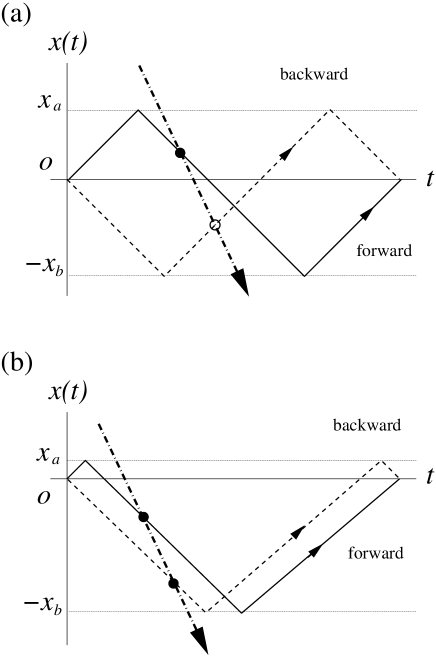
Figure 14: World lines corresponding to the time-reversed trajectories (solid and dashed lines) with velocity $v^{*}$ in the three-impurity Cooperon. The dash-dotted line describes the propagation of a plasmon with velocity $u$. (a) Regular configuration (Sec. IV) contributing to $\Delta\sigma_{\rm WL}$; (b) asymmetric configuration (Sec. V) contributing to $\Delta\sigma_{\rm ME}$. The interaction line gives a contribution to the dephasing action $S$ which is proportional to $\alpha(N_{f}-N_{b})^{2}$. Here $N_{f,b}$ is the number of the small-angle intersections (black dots) of a plasmon line with the forward ($f$) and backward ($b$) paths. The intersections at a large angle (the plasmon and electrons moving in opposite directions, unfilled circles) contribute to the dephasing only at second order in $\alpha$ and hence are neglected. One sees that $N_{f}\neq N_{b}$ for typical configurations (a), whereas for asymmetric configurations (b) $N_{f}=N_{b}$ for most of the plasmon lines. For a corresponding plot in the spinless case, see Fig. 7 of Ref. GMP, .

Since the dominant contribution to the dephasing rate is given by the $g_{4}$–processes of scattering between electrons from the same chiral branch, we will set $g_{2}=0$ which is consistent with our central approximation $\alpha_{b}\to 0$. Furthermore, it is convenient to introduce different coupling constants, sol79 ; voit94 $g_{4}^{\parallel}$ and $g_{4}^{\perp}$, for interaction between electrons with equal and opposite spins, respectively (at the end, we set $g_{4}^{\parallel}=g_{4}^{\perp}=g\simeq 2\pi v\alpha$). In view of the Pauli principle, the $g_{4}^{\parallel}$–interaction does not lead to any real scattering but only renormalizes the velocity of electrons:

$$v\to v^{*}=v(1+g_{4}^{\parallel}/2\pi v)~{}.$$ (6.1)

This allows us to put $g_{4}^{\parallel}=0$, simultaneously replacing $v$ by $v^{*}$. All the nontrivial interaction-induced physics is due to $g_{4}^{\perp}$–processes.

Solving the corresponding RPA equations for the interaction propagators, we get for parallel ($V^{\parallel}$) and anti-parallel ($V^{\perp}$) spins :

$$V_{++}^{\perp}(q,\omega) = 2\pi v^{*}\alpha{(v^{*}q-\omega)^{2}\over(uq-\omega)(vq-\omega)},$$

$$V_{++}^{\parallel}(q,\omega) = -2\pi v^{*}\alpha^{2}{v^{*}q(v^{*}q-\omega)\over(uq-\omega)(vq-\omega)}$$ (6.2)

and

$$V^{\perp(\parallel)}_{--}(q,\omega)=V^{\perp(\parallel)}_{++}(-q,\omega)~{},$$ (6.3)

where $u=v(1+2\alpha)$ and $v^{*}=v(1+\alpha)$. We note that $V^{\perp}$ does not enter the path integral, since electron spin is conserved.

The general expression for the WL dephasing action acquired on the exactly time-reversed trajectories $x_{\rm b}(t)=x_{\rm f}(t_{C}-t)$ for the three-impurity Cooperon reads GMPlett ; GMP

$$S_{ij}(t_{C},\{x(t)\})\!=\!-T\int_{0}^{t_{C}}\!dt_{1}\int_{0}^{t_{C}}\!dt_{2}\int{d\omega\over 2\pi}\int{dq\over 2\pi}$$

$$\times{{\rm Im}V^{\parallel}_{\mu\nu}(q,\omega)\over\omega}\exp\left\{iq[\,x_{i}(t_{1})-x_{j}(t_{2})]-i\omega[t_{1}-t_{2}]\right\}$$

$$=\!-T\int_{0}^{t_{C}}\!dt_{1}\int_{0}^{t_{C}}\!dt_{2}\,{\cal F}^{\parallel}_{\mu\nu}[x_{i}(t_{1})-x_{j}(t_{2}),\,t_{1}-t_{2}]~{},$$

where each of the indices $i,j$ takes one of the values “${\rm f}$” (for the forward path of the Cooperon) or “${\rm b}$” (for the backward path), $\mu={\rm sgn}{\dot{x}}_{i}$ and $\nu={\rm sgn}{\dot{x}}_{j}$, and ${\cal F}^{\parallel}_{\mu\nu}(x,t)$ is the Fourier transform of $\omega^{-1}{\rm Im}V^{\parallel}_{\mu\nu}(q,\omega)$. The main contribution comes from the diagonal terms with $i=j$ and $t_{1}=t_{2}$, for which $\mu=\nu$, see Fig. 14a. The imaginary part of the corresponding interaction propagator is written as

$${\rm Im}\,V_{\pm\pm}^{\parallel}(q,\omega) = (\pi v^{*}\alpha)^{2}{\omega\over uv}$$ (6.5)

$$\times \left[\ u\,\delta(vq\mp\omega)+v\,\delta(uq\mp\omega)\right],$$

which gives

$${\cal F}^{\parallel}_{\pm\pm}(x,t)=-\pi\,{(v^{*}\alpha)^{2}\over 2uv}\,\left[\,u\,\delta(x\mp vt)+v\,\delta(x\mp ut)\,\right].$$

(6.6)

A graphic illustration of the e-e scattering processes contributing to the dephasing action $S=2(S_{\rm ff}-S_{\rm fb})$ is presented in Fig. 14. There, we show by the circles and black dots the space-time coordinates for which the arguments of the $\delta$-functions in Eq. (6.6) are zero. The main contribution to $S$ comes from small-angle intersections (black dots). For electron trajectories characterized by velocity $v^{*}$, these give a large factor of the order of $\alpha^{-1}$, either $v^{*}/|u-v^{*}|$ or $v^{*}/|v-v^{*}|$ [cf. Eq. (2.14)]. As a result, the action for typical impurity configurations (Fig. 14a) reads

$$S\sim\alpha^{2}Tt_{C}/|\alpha|\sim|\alpha|Tt_{C}.$$ (6.7)

For comparison, in the spinless caseGMPlett ; GMP , intersections between the interaction and particle propagators running in the same direction give zero dephasing because of the cancellation between the Hartree and exchange terms (Sec. II.2). On the other hand, at large angles the ballistic (straight line) interaction propagator always intersects a pair of (forward and backward) electron trajectories, which gives zero dephasing as well. As a result, only the intersections at large angles that arise from scattering of the interaction propagator off disorder contribute to the dephasing rate.GMPlett ; GMP

More rigorously, substituting Eq. (6.6) in Eq. (VI), we find the dephasing action for the trajectory characterized by the velocity $v^{*}$,

$$S\simeq\frac{8\pi T}{v}\left\{\begin{array}[]{ll}x_{a},&\quad 0<x_{a}<\alpha x_{c}/2~{},\\[5.69054pt] \alpha x_{c}/2,&\quad\alpha x_{c}/2<x_{a}<(1-\alpha/2)\,x_{c}~{},\\[5.69054pt] x_{c}-x_{a},&\quad(1-\alpha/2)\,x_{c}<x_{a}<x_{c}~{},\end{array}\right.$$ (6.8)

which is illustrated in Fig. 15. Any other velocity between $v$ and $u$ yields a qualitatively similar action, but with different numerical factors. This is another indication of the previously discussed fact that all velocities from this interval contribute to the conductivity correction.

Figure 15: Dephasing action $S$ (in units of $2x_{c}/l_{ee}$) corresponding to the velocity $v^{*}$, Eq. (6.8), as a function of $x_{a}$ for fixed $x_{c}$.

One sees from Eq. (6.8) (middle line) and Fig. 15 (flat region) that for typical impurity configurations the dephasing action becomes of the order of unity at $t_{C}=2x_{c}/v^{*}\sim 1/\alpha T$. This gives a parametric estimate for the dephasing length $l_{\phi}\sim\alpha^{-1}l_{T}$, and for the WL correction $\Delta\sigma_{\rm WL}/\sigma_{\rm D}\sim-(l_{ee}/l)^{2}$, in agreement with the results of Sec. IV. Equation (6.8) (first and third lines) and Fig. 15 also demonstrate the suppression of the dephasing action in the anomalous (strongly asymmetric) impurity configurations (Fig. 14b) responsible for the ME, $\Delta\sigma_{\rm ME}/\sigma_{\rm D}\sim-l_{T}/l$, as discussed in Sec. V.

VII Summary

	e-e scattering	dephasing	WL correction	ME correction
	length $l_{ee}$	length $l_{\phi}$	$\Delta\sigma_{\rm WL}/\sigma_{\rm D}$	$\Delta\sigma_{\rm ME}/\sigma_{\rm D}$
spinless
	$\displaystyle{{v\over\alpha^{2}T}}$	$\displaystyle{{1\over\alpha}\left({{vl\over T}}\right)^{1/2}}$	$\displaystyle{-\Big{(}{l_{\phi}\over l}\Big{)}^{2}\ln{l\over l_{\phi}}\sim-{v\ln(\alpha^{2}Tl/v)\over\alpha^{2}Tl}}$	$\displaystyle{-{l_{ee}\over l}\sim-{v\over\alpha^{2}Tl}}$
spinful
	$\displaystyle{{v\over\alpha T}}$	$\displaystyle{{v\over\alpha T}}$	$\displaystyle{-\Big{(}{l_{\phi}\over l}\Big{)}^{2}\sim-\Big{(}{v\over\alpha Tl}\Big{)}^{2}}$	$\displaystyle{-{l_{T}\over l}\sim-{v\over Tl}}$

Table 1: Characteristic spatial scales induced by interaction and the conductivity corrections for spinless and spinful disordered LLs.

To conclude, we have analyzed, within the functional bosonization formalism, the quantum interference of interacting electrons in a disordered spinful LL. Our results are summarized in Table 1 and in Fig. 16.

The single-particle properties of fermionic excitations in this model have been studied in Sec. III in several representations. Two most important and interrelated features of the single-particle spectral characteristics are: (i) the SCS, as a result of which the whole range of velocities between the charge velocity $u$ and the spin velocity $v$ contributes to the spectral function, and (ii) the single-particle decay on the spatial scale of $l_{ee}$, Eq. (3.9).

In Sec.IV we have calculated the leading quantum interference correction to the conductivity, Eq. (4.25). The corresponding dephasing length $l_{\phi}$ is given by Eq. (4.28). Two qualitative differences as compared to the spinless case should be emphasized in this context. Firstly, for spinful electrons, the decay length of single-particle excitations is inversely proportional to the first order in the interaction strength $\alpha$, $l_{ee}\sim\alpha^{-1}l_{T}$, whereas $l_{ee}\sim\alpha^{-2}l_{T}$ in the absence of spin. Secondly, the WL dephasing length $l_{\phi}$ is equal to the single-particle dephasing length $l_{ee}$ in the spinful model, whereas $l_{\phi}$ depends on the strength of disorder, $l_{\phi}\sim\sqrt{l_{ee}l}$, for spinless electrons.

In Sec. V we have analyzed the contribution to the Cooperon diagrams of “nontypical” configurations of disorder with two impurities being anomalously close to each other. We have shown that this contribution, Eq. (5.16), describes the quasiclassical ME. It is parametrically smaller than the WL term at sufficiently low $T$ and gives the leading correction to the conductivity in the limit of high $T$.

Figure 16: Schematic plot (log-log scale) of the $T$ dependence of the conductivity $\sigma(T)$ of spinful electrons.

Our findings, demonstrating the strong dependence of the quantum interference effects on spin in a LL, imply that the Zeeman splitting by magnetic field should lead to strong effects in the conductivity of a single-channel quantum wire. Results obtained in this direction will be reported elsewhere.magres

We thank D. Aristov, D. Bagrets, and A. Morpurgo for useful discussions and gratefully acknowledge support by EUROHORCS/ESF (AGY and IVG), by the DFG Center for Functional Nanostructures, and by RFBR [Grant No. 06-02-16702] (AGY).

References

- (1) J. Sólyom, Adv. Phys. 28, 201 (1979).
- (2) J. Voit, Rep. Prog. Phys. 57, 977 (1994).
- (3) H.J. Schulz, in Mesoscopic Quantum Physics, edited by E. Akkermans, G. Montambaux, J.-L. Pichard, and J. Zinn-Justin (North-Holland, Amsterdam, 1995).
- (4) A.O. Gogolin, A.A. Nersesyan, and A.M. Tsvelik, Bosonization and Strongly Correlated Systems (Cambridge University Press, Cambridge, England, 1998).
- (5) H.J. Schulz, G. Cuniberti, and P. Pieri, in Field Theories for Low-Dimensional Condensed Matter Systems, edited by G. Morandi, P. Sodano, P. Tagliacozzo, and V. Tognetti (Springer, Berlin, 2000).
- (6) D.L. Maslov, in Nanophysics: Coherence and Transport, edited by H. Bouchiat, Y. Gefen, S. Guéron, G. Montambaux, and J. Dalibard (Elsevier, Amsterdam, 2005); cond-mat/0506035.
- (7) T. Giamarchi, Quantum Physics in One Dimension (Oxford University Press, Oxford, 2004).
- (8) M. Bockrath, D.H. Cobden, J. Lu, A.G. Rinzler, R.E. Smalley, L. Balents, and P.L. McEuen, Nature 397, 598 (1999); J. Nygård, D.H. Cobden, and P.E. Lindelof, ibid. 408, 342 (2000); J. Wei, M. Shimogawa, Z. Wang, I. Radu, R. Dormaier, and D.H. Cobden, Phys. Rev. Lett. 95, 256601 (2005); P.J. Leek, M.R. Buitelaar, V.I. Talyanskii, C.G. Smith, D. Anderson, G.A.C. Jones, J. Wei, and D.H. Cobden, ibid. 95, 256802 (2005).
- (9) Z. Yao, H. Postma, L. Balents, and C. Dekker, Nature 402, 273 (1999); Z. Yao, C.L. Kane, and C. Dekker, Phys. Rev. Lett. 84, 2941 (2000); H.W.Ch. Postma, T. Teepen, Z. Yao, M. Grifoni, and C. Dekker, Science 293, 76 (2001).
- (10) A.F. Morpurgo, J. Kong, C.M. Marcus, and H. Dai, Science 286, 263 (1999); N. Mason, M.J. Biercuk, and C.M. Marcus, ibid., 303, 655 (2004).
- (11) A.Y. Kasumov, R. Deblock, M. Kociak, B. Reulet, H. Bouchiat, I.I. Khodos, Yu.B. Gorbatov, V.T. Volkov, C. Journet, and M. Burghard, Science 284, 1508 (1999); P. Jarillo-Herrero, J.A. van Dam, and L.P. Kouwenhoven, Nature 439, 953 (2006).
- (12) H.R. Shea, R. Martel, and Ph. Avouris, Phys. Rev. Lett. 84, 4441 (2000).
- (13) R. Krupke, F. Hennrich, H.B. Weber, D. Beckmann, O. Hampe, S. Malik, M.M. Kappes, and H. v. Löhneysen, Appl. Phys. A 76, 397 (2003).
- (14) H.T. Man, I.J.W. Wever, and A.F. Morpurgo, Phys. Rev. B 73, 241401 (2006).
- (15) O.M. Auslaender, A. Yacoby, R. de Picciotto, K.W. Baldwin, L.N. Pfeiffer, and K.W. West, Phys. Rev. Lett. 84, 1764 (2000); Science 295, 825 (2002); O.M. Auslaender, H. Steinberg, A. Yacoby, Y. Tserkovnyak, B.I. Halperin, K.W. Baldwin, L.N. Pfeiffer, and K.W. West, ibid. 308, 88 (2005).
- (16) S.V. Zaitsev-Zotov, Y.A. Kumzerov, Y.A. Firsov, and P. Monceau, J. Phys. Cond. Matter 12, L303 (2000); Pis’ma v ZhETF 77, 162 (2003) [JETP Lett. 77, 135 (2003)]; E. Levy, A. Tsukernik, M. Karpovski, A. Palevski, B. Dwir, E. Pelucchi, A. Rudra, E. Kapon, and Y. Oreg, Phys. Rev. Lett. 97, 196802 (2006).
- (17) Y. Jompol, C.J.B. Ford, I. Farrer, G.A.C. Jones, D. Anderson, D.A. Ritchie, T.W. Silk, and A.J. Schofield, Physica E 40, 1220 (2008).
- (18) W.K. Hew, K.J. Thomas, M. Pepper, I. Farrer, D. Anderson, G.A.C. Jones, and D.A. Ritchie, Phys. Rev. Lett. 101, 036801 (2008).
- (19) E. Slot, M.A. Holst, H.S.J. van der Zant, and S.V. Zaitsev-Zotov, Phys. Rev. Lett. 93, 176602 (2004); L. Venkataraman, Y.S. Hong, and P. Kim, ibid. 96, 076601 (2006).
- (20) A.N. Aleshin, H.J. Lee, Y.W. Park, and K. Akagi, Phys. Rev. Lett. 93, 196601 (2004); A.N. Aleshin, Adv. Mat. 18, 17 (2006).
- (21) W. Kang, H.L. Stormer, L.N. Pfeiffer, K.W. Baldwin, and K.W. West, Nature 403, 59 (2000); I. Yang, W. Kang, K.W. Baldwin, L.N. Pfeiffer, and K.W. West, Phys. Rev. Lett. 92, 056802 (2004).
- (22) M. Grayson, D. Schuh, M. Huber, M. Bichler, and G. Abstreiter, Appl. Phys. Lett. 86, 032101 (2005); M. Grayson, L. Steinke, D. Schuh, M. Bichler, L. Hoeppel, J. Smet, K. v. Klitzing, D.K. Maude, and G. Abstreiter, Phys. Rev. B 76, 201304 (2007); L. Steinke, D. Schuh, M. Bichler, G. Abstreiter, and M. Grayson, ibid. 77, 235319 (2008).
- (23) I. Bloch, J. Dalibard, and W. Zwerger, Rev. Mod. Phys. 80, 885 (2008).
- (24) H.T. Man and A.F. Morpurgo, Phys. Rev. Lett. 95, 026801 (2005).
- (25) S. Li, Z. Yu, C. Rutherglen, and P.J. Burke, Nano Lett. 4, 2003 (2004).
- (26) M. Purewal, B.H. Hong, A. Ravi, B. Chandra, J. Hone, and P. Kim, Phys. Rev. Lett. 98, 186808 (2007); B.H. Hong, J.Y. Lee, T. Beetz, Y. Zhu, P. Kim, and K.S. Kim, J. Am. Chem. Soc. 127, 15336 (2005).
- (27) I.V. Gornyi, A.D. Mirlin, and D.G. Polyakov, Phys. Rev. Lett. 95, 046404 (2005).
- (28) I.V. Gornyi, A.D. Mirlin, and D.G. Polyakov, Phys. Rev. B 75, 085421 (2007).
- (29) T. Micklitz, A. Altland, and J.S. Meyer, arXiv:0805.3677.
- (30) The regime of strong localization emerging at lower temperatures is outside the scope of the present work [see, e.g., L. Fleishman and P.W. Anderson, Phys. Rev. B 21, 2366 (1980); I.V. Gornyi, A.D. Mirlin, and D.G. Polyakov, Phys. Rev. Lett. 95, 206603 (2005); D.M. Basko, I.L. Aleiner, and B.L. Altshuler, Ann. Phys. (N.Y.) 321, 1126 (2006)].
- (31) K. Le Hur, Phys. Rev. B 65, 233314 (2002).
- (32) K. Le Hur, Phys. Rev. Lett. 95, 076801 (2005); Phys. Rev. B 74, 165104 (2006).
- (33) D.B. Gutman, Y. Gefen, and A.D. Mirlin, arXiv:0804.4294, to appear in Phys. Rev. Lett.
- (34) For review see G.A. Fiete, Rev. Mod. Phys. 79, 801 (2007).
- (35) K.A. Matveev, Phys. Rev. Lett. 92, 106801 (2004); Phys. Rev. B 70, 245319 (2004).
- (36) G.A. Fiete and L. Balents, Phys. Rev. Lett. 93, 226401 (2004); G.A. Fiete, K. Le Hur, L. Balents, Phys. Rev. B 72, 125416 (2005).
- (37) V.V. Cheianov and M.B. Zvonarev, Phys. Rev. Lett. 92, 176401 (2004); J. Phys. A 37, 2261 (2004); M.B. Zvonarev, V.V. Cheianov, and T. Giamarchi, Phys. Rev. Lett. 99, 240404 (2007).
- (38) See, e.g., G. Baym and C. Pethick, Landau Fermi-liquid theory (Wiley-VCH, Weinheim, 2004).
- (39) The SCS manifests itself in a nontrivial way also in the bosonic (density-density) response function at the wavector , where is the Fermi wavevector, see A. Iucci, G.A. Fiete, and T. Giamarchi, Phys. Rev. B 75, 205116 (2007).
- (40) Neglecting is not always justified despite being much smaller than . First, in the presence of spin, -processes “added” to the clean LL model are a “marginally relevant” or “marginally irrelevant” perturbation in the renormalization-group sense, depending on the sign of the bare (see, e.g., Refs. sol79, ; voit94, ). For repulsive Coulomb interaction (), weak backward e-e scattering is marginally irrelevant, i.e., only leads to a small renormalization of the effective couplings of the LL theory on (exponentially) large spatial scales. We neglect the weak renormalization due to -processes altogether. Second, there exist phenomena which are entirely due to -processes. One of these is the spin-related magnetoresistance of a single-channel quantum wire,matveev93 ; magres which we will consider elsewhere.magres However, for the effects studied in the present paper, it suffices to deal with forward e-e scattering only.
- (41) K.A. Matveev, D. Yue, and L.I. Glazman, Phys. Rev. Lett. 71, 3351 (1993); D. Yue, L.I. Glazman, and K.A. Matveev, Phys. Rev. B 49, 1966 (1994).
- (42) A.G. Yashenkin, I.V. Gornyi, A.D. Mirlin, and D.G. Polyakov, in preparation.
- (43) A.A. Abrikosov and I.A. Ryzhkin, Adv. Phys. 27, 147 (1978).
- (44) I.E. Dzyaloshinskii and A.I. Larkin, Zh. Éksp. Teor. Fiz. 65, 411 (1973) [Sov. Phys. JETP 38, 202 (1974)].
- (45) H.C. Fogedby, J. Phys. C 9, 3757 (1976).
- (46) D.K.K. Lee and Y. Chen, J. Phys. A 21, 4155 (1988).
- (47) I.V. Yurkevich, in Strongly Correlated Fermions and Bosons in Low-Dimensional Disordered Systems, edited by I.V. Lerner, B.L. Altshuler, and V.I. Fal’ko (Kluwer, Dordrecht, 2002), cond-mat/0112270; I.V. Lerner and I.V. Yurkevich, in Nanophysics: Coherence and Transport, edited by H. Bouchiat, Y. Gefen, S. Guéron, G. Montambaux, and J. Dalibard (Elsevier, Amsterdam, 2005), cond-mat/0508223; A. Grishin, I.V. Yurkevich, and I.V. Lerner, Phys. Rev. B 69, 165108 (2004).
- (48) P. Kopietz, Bosonization of Interacting Electrons in Arbitrary Dimensions (Springer, Berlin, 1997)
- (49) C.M. Naón, M.C. von Reichenbach, and M.L. Trobo, Nucl. Phys. B 435, 567 (1995); V. Fernández, K. Li, and C. Naón, Phys. Lett. B 452, 98 (1999); V.I. Fernández and C.M. Naón, Phys. Rev. B 64, 033402 (2001); C. Naón, M.J. Salvay, M.L. Trobo, Int. J. Mod. Phys. A19, 4953 (2004).
- (50) U. Eckern and P. Schwab, phys. stat. sol. (b) 244, 2343 (2007).
- (51) D.A. Bagrets, I.V. Gornyi, and D.G. Polyakov, unpublished.
- (52) D.A. Bagrets, I.V. Gornyi, A.D. Mirlin, and D.G. Polyakov, Semiconductors 42, 994 (2008).
- (53) This approximation is exact for a spinful chiral LL in which .
- (54) J. Voit, Phys. Rev. B 47, 6740 (1993).
- (55) V. Meden and K. Schönhammer, Phys. Rev. B 46, 15753 (1992).
- (56) D.C. Mattis, Phys. Rev. Lett. 32, 714 (1974).
- (57) A. Luther and I. Peschel, Phys. Rev. Lett. 32, 992 (1974).
- (58) T. Giamarchi and H.J. Schulz, Phys. Rev. B 37, 325 (1988).
- (59) C.L. Kane and M.P.A. Fisher, Phys. Rev. Lett. 68, 1220 (1992); Phys. Rev. B 46, 15233 (1992).
- (60) See, e.g., J. Wilke, A.D. Mirlin, D.G. Polyakov, F. Evers, and P. Wölfle, Phys. Rev. B 61, 13774 (2000) and references therein.
- (61) Under the conditions (5.1) and (5.2), interaction drops out of the problem only within the approximation (4.5), corresponding to . The omitted factors with the exponent in make time-dependent, which results in the renormalization of impurities—already taken into account in Eq. (4.2).
- (62) This should be contrasted with the regular configurations, where adding two lines (only diagrams with an odd number of impurity backscattering lines contribute to the Cooperon) multiplies the result for the conductivity by a small paramter , in view of dephasing.
- (63) B.L. Altshuler, A.G. Aronov, and D.E. Khmelnitskii, J. Phys. C 15, 7367 (1982).