Explosive Events and the Evolution of the Photospheric Magnetic Field

Abstract

Transition region explosive events have long been suggested as direct signatures of magnetic reconnection in the solar atmosphere. In seeking further observational evidence to support this interpretation, we study the relation between explosive events and the evolution of the solar magnetic field as seen in line–of–sight photospheric magnetograms. We find that about 38% of events show changes of the magnetic structure in the photosphere at the location of an explosive event over a time period of 1 h. We also discuss potential ambiguities in the analysis of high sensitivity magnetograms.

1 Introduction

Explosive events (EEs) are defined by strong transient enhancements of the wings of spectral lines that form at transition region (TR) temperatures. They were first observed with the rocket–borne High Resolution Telescope and Spectrograph (HRTS) flown by the Naval Research Laboratory (Brueckner & Bartoe 1983; Dere et al. 1984). The physical properties of EEs as derived from the HRTS flights are described in Dere (1994, Table 1): time scales between 20-200s (with an average of 60s), spatial scales of around 1500 km ($\approx$2^′′) and velocities of about 100 km ${\rm s^{-1}}$. They are best seen in TR emission lines produced at temperatures of $2\times 10^{4}-2\times 10^{5}$ K. Spatial maps derived from raster sequences showed that EEs can be found all over the quiet Sun, including at the limb and in coronal holes. Wing enhancements were not always symmetric, sometimes only a red or blue wing was present, often having a spatial offset of 1^′′-2^′′ along the slit.

More recent studies have analysed spectra from the Solar Ultraviolet Measurements of Emitted Radiation (SUMER, Wilhelm et al. 1995) instrument onboard the Solar and Heliospheric Observatory (SoHO). Pérez & Doyle (2000) summarize the properties of EEs derived from SUMER spectra, based on a small sample of 8 events. Earlier HRTS results are largely confirmed, with some variations due to the different characteristics of the SUMER instrument (see also Teriaca et al. 2004). For instance, lifetimes are longer, probably due to the longer exposure times needed by SUMER, while sizes are larger (4^′′–14^′′) due to the lower spatial resolution of SUMER compared to HRTS.

Part of the interest in the study of EEs stems from the idea that they could be an important indicator of heating and/or acceleration processes in the upper solar atmosphere. To determine the origin of EEs and evaluate their contribution to the mass and energy flux in the solar atmosphere, one must address the question of their relationship with the magnetic field topology. Porter & Dere (1991) found that most EEs are located near the magnetic network, which was confirmed later, e.g. by Moses et al. (1994) and Chae et al. (1998). The TR line emission of EEs is usually fainter than the enhanced emission that corresponds to the magnetic network. This is one of the important differences between EEs and other small–scale transients of the solar TR and corona. For example, coronal and X-ray bright points are found directly within the bright network and exhibit enhanced X-ray and EUV emission, with sizes of about 10^′′ – 40^′′ and lifetimes between several hours and 1–2 days. They consist of small–scale arcades of loops connecting opposite polarities of small magnetic bipoles (e.g. Sheeley & Golub 1979; Habbal 1992; Webb et al. 1993; Madjarska et al. 2003). In contrast, EEs are usually not seen in coronal lines, but are limited to lines at TR temperatures.

Another TR phenomenon which was discovered with Coronal Diagnostic Spectrometer (CDS) on SoHO are the so-called blinkers (e.g. Harrison 1997, Bewsher et al. 2002). They are best observed in transition region lines like O IV 554 Å ($1.6\times 10^{5}$ K) and O V 629 Å ($2.5\times 10^{5}$ K). These events are characterized by an intensity enhancement factor of about 1.2 to 2.7 and a duration of around 1 to 40 min (although some of the longer ones seem to be composed of short–duration elementary blinkers, according to Brooks et al. 2004). Like EEs, blinkers do not appear to have any detectable coronal or chromospheric signatures. Bewsher et al. (2002) found that most blinkers are located above regions of strong flux, the magnetic network.

The relationship between EEs and TR blinkers has been examined in several studies. Based on a statistical analysis Brković & Peter (2004) concluded that explosive events and blinkers are independent phenomena. Bewsher et al. (2005) raise doubts as to a link between them and their probability analysis shows that such a link is very unlikely. Madjarska & Doyle (2003) described the main characteristics of both EEs and blinkers that imply that they are more likely two separate phenomena not directly related or triggering each other. On the other hand, Chae et al. (2000) have put forth the idea that blinkers “consist of many small–scale and short–lived SUMER unit brightening events having sizes and durations that are very comparable to those of explosive events”. They attribute the difference in spectral characteristics of blinkers and EEs to different magnetic geometries involved in the underlying reconnection. This controversy clearly underscores the importance of studying the magnetic field structure of EEs and other small-scale TR phenomena.

The basic mechanism proposed for the formation of EEs is magnetic reconnection taking place near the magnetic network. Dere et al. (1991, their Fig. 2) illustrates this in a schematic way. Patches of bipolar magnetic flux emerge in the interiors of the supergranular cells and are swept to the boundaries by the supergranular flow. If a network element has the opposite polarity, the flux will eventually come close enough for reconnection to occur. The intense wing broadening of the spectral lines is thought to be due to plasma that is accelerated in the reconnection process (Innes et al. 1997). In this scenario the EEs are therefore considered to be a direct consequence of magnetic reconnection in the TR.

From the spatial distribution of EEs superposed on a map that displays the chromospheric network it can be seen that EEs not only seem to avoid the magnetic network, but are also rarely located in the centers of supergranular cells (e.g. Porter & Dere 1991). The work of Porter & Dere (1991) was limited to a comparison of EE locations with single magnetograms taken at the time of the HRTS flights. Therefore, the temporal evolution of the magnetic field could not be addressed.

Some of the early observations with HRTS showed some associations of EEs with emerging flux regions, as in the case of HRTS-6 (Dere et al. 1991). For the HRTS-7 flight magnetograms from several ground–based observatories were available. In one case an EE was found to be connected to a small emerging bipole that later merged with a pre-existing patch of nearby flux (Dere & Martin 1994). Many more EEs were found in quiet sun regions, but no simultaneous magnetic field measurements were available. Therefore, the case for interpreting EEs as evidence for reconnection during magnetic flux emergence has been largely circumstantial.

A detailed account of the magnetic field evolution in connection with EEs is given by Chae et al. (1998). They compared SUMER EEs with deep magnetograms taken at Big Bear Solar Observatory (BBSO). They found that EEs are located near the magnetic network (in agreement with Porter & Dere 1991). Out of a total of 163 EEs in their spectroheliogram, 103 are at a location of flux cancellation. Section 4 discusses their results in more detail.

More recently, Madjarska & Doyle (2003) used data from SUMER, CDS and BBSO and were unable to associate EEs with any particular magnetic field pattern. On the other hand they found that blinkers are associated with bipolar magnetic regions, although they found no flux cancellation or changes in total flux for blinkers.

A different approach to a closely related topic was presented by Sanchez Almeida et al. (2007). Their work illustrated an attempt to find footpoints of quiet Sun TR loops using G–band bright points. These are used as proxies for photospheric magnetic field concentrations which may anchor and guide the TR structures. They also identified several EEs in their SUMER data, but found a tendency that EEs avoided G–band bright points. As explained in our standard scenario above, we consider EEs are the direct signature of reconnection taking place in the TR. On the other hand Tarbell et al. (2000) proposed reconnection in the photosphere, which leads to shocks and shock interaction that accelerate the plasma at TR temperatures. Sanchez Almeida et al. (2007) argued that, if G–band bright points are footpoints of loops undergoing reconnection, then the fact that the EEs do not coincide with them indicates that the site of TR plasma acceleration is far from the photospheric footpoints.

The purpose of the current study is to identify signatures of EEs in the underlying photospheric magnetic field and to illuminate the role of magnetic reconnection in the formation of EEs. The following section describes the observations and basic data analysis. Section 3 shows the results of our combined data and Section 4 discusses the magnetic field evolution.

2 Observations and Data Processing

In our analysis we combine data from two instruments onboard SoHO. Until recently the SUMER instrument was the only instrument in operation that was able to identify EEs by their spectral signature. The Michelson Doppler Imager (MDI, Scherrer et al. 1995) can continuously map a large disk fraction of photospheric magnetic field with moderate to good spatial resolution over many hours. The data have been taken on 7th November 1999, they have been taken strictly simultaneously and cospatiality is ensured by the data processing. With this combination of instruments we have the opportunity to study the relation of EEs and the underlying magnetic field in unprecedented detail.

2.1 SUMER

The SUMER instrument onboard SoHO was designed to observe spectral lines in the range from around 500 Å to 1610 Å. This study employs data obtained in the scanning mode in order to allow coalignment of the SUMER data with the MDI magnetograms. SUMER was taking data around 1550 Å, which covered two C IV lines (1548 Å, and 1550 Å, formation temperature $1\times 10^{5}$ K), a Si II line (1533 Å, $1.8\times 10^{4}$ K) and a Ne VIII line (770 Å in the second order, $6.3\times 10^{5}$ K). Figure 1 shows an example of a C IV spectrum, including several spectral profiles of EEs. Exposure times were 150 s and SUMER performed 60 raster steps each of 3^′′ (nominally). This scan was repeated 3 times. Only the first scan and part of the second had co-temporal MDI data and are considered in this analysis. Spatial sampling along the SUMER slit corresponds to approximately 1^′′/pixel.

Basic data processing of the raw SUMER spectra includes decompression, flat–fielding and geometrical corrections. We note that the destretching algorithm that is available with the public software uses pre-flight calibration data and does not work perfectly. Residual image distortions are still present and are worst at the edges of the detector. Finally, we fit the line profiles with a single Gaußian to obtain integrated intensity, central wavelength and width of the spectral lines.

The characteristic signature of an EE is enhanced emission in the wings of the spectral line. We developed the following algorithm to identify such wing enhancements. We first determine the continuum in a nearby wavelength range and the root mean square (rms) of the continuum $I_{\rm rms}$. We then smooth the spectra in wavelength and determine the location of the maximum emission in the C IV 1548 Å line. We exclude locations where the maximum of the emission is less than 10$\times I_{\rm rms}$ and where the continuum is less than 1. Thus, the algorithm avoids very weak profiles that mostly consist of noise. We note that these criteria automatically remove most locations in the centers of network cells. Therefore our algorithm is biased against finding EEs in cell centers. Finally, we calculate the average intensity between 70–130 km ${\rm s^{-1}}$(5 spectral pixels) to the red and blue of the line center. If this value is larger than 0.3 times the maximum intensity of the line, the line profile will be flagged as a potential EE. In the last step, the flagged spectra are displayed and the final determination is done visually.

Our algorithm is designed to reject moderately enhanced (less than 30% of the line maximum) and moderately broadened (velocities $<$ 70 km ${\rm s^{-1}}$) line profiles. While such profiles exist, they are generally not included in our analysis. In the case of rather weak lines the 30% criterion removes profiles where the wing enhancements are also near the noise level. On the other hand, we found several cases where the central component of the line was very strong and a very clear wing enhancement was present, but the 30% criterion was not fulfilled due to the brightness of the central component. We have added these locations to our sample of EEs by hand.

In agreement with the known size of EEs, characteristic wing enhancements are often found in more than one pixel along the slit and sometimes also in neighbouring scan positions. If an event covers several pixels, all adjacent pixels are counted as one single event.

2.2 MDI

We use magnetograms and Dopplergrams that were taken in the high resolution (HR) mode of MDI. These data have a spatial sampling of 0.6^′′ per pixel, and one set of observables is obtained every minute.

The data used in this study are available from the MDI web archive. and have been processed to the 1.8 level. Raw data from the spacecraft have first been calibrated into physical units of the observable and time and location of the observation. Descriptive and ancillary data have been added and finally level 1.8 processing went on to provide time–dependent corrections for plate scale, zero offset, sensitivity, and cosmic rays. We checked the sequences for missing images and used linear interpolation from adjacent ones to fill data gaps.

It takes 30 s to measure the 5 filter locations in the Ni I 6768 Å line from which magnetograms, Dopplergrams and intensity images are derived. According to Scherrer et al. (1995) a single longitudinal magnetogram has a 1$\sigma$ noise level of 20 Mx cm^-2. At least part of the noise in the magnetograms can be attributed to cross-talk of the velocity signal into the magnetic signal (e.g. Settele et al. 2002). During the time MDI needs to measure the 5 filter positions (30 s), the spectral line is also shifted in wavelength due to the photospheric velocity field. The magnetic signal is calculated from differences of filtergrams in the two polarization states, and the Doppler shift introduces such differences over the exposure time.

We carry out a 3–D Fourier transformation of our quiet Sun MDI magnetogram sequences. In the resulting $k{-}\omega$ diagram variations with characteristic time scales of 2–5 min are present which are due to wave motions. To remove the effect of oscillations in our magnetograms, we apply a subsonic Fourier filter with a cutoff phase velocity of $v_{ph}$ = 3 km ${\rm s^{-1}}$. Close inspection of the filtered magnetogram sequences reveals the presence of fluctuations on granular scales. As we expect the changes in magnetic flux associated with EEs to be small, we refrain from additional spatial and/or temporal averaging.

To determine the noise in the filtered magnetograms we follow the method of Hagenaar (2001) and Parnell (2002). A histogram of the magnetic flux of various selected regions was fit with a Gaußian centered on the zero value. From this analysis we derive a value of $B=\pm$ 9 Mx cm^-2 as the one sigma noise level. We disregard all flux between these values by setting it to zero.

We apply the same analysis procedure to the MDI Dopplergrams. The rms of the Doppler fluctuations of a filtered data-cube is around 150 m ${\rm s^{-1}}$, with a peak–to–peak amplitude of about $\pm$ 600 m ${\rm s^{-1}}$.

2.3 Combining SUMER and MDI data

Because EEs have very small spatial scales, proper co–alignment of SUMER with MDI is critical. Both the SUMER scan and MDI magnetograms have to be scaled to the same size and then cross-correlated. The fact that SUMER is scanning while MDI takes a series of snapshots complicates the analysis further due to the evolution of the solar structures.

SUMER scanning is carried out either from east to west or from west to east. Depending on whether or not the scan is in the sense of the Sun’s rotation, the observed field of view (FOV) is either smaller or larger. The smallest scan step that can be carried out with the scanning mechanism is 0.38^′′, so a complete scan step of 3^′′ requires 8 elementary steps. After 1997 the scanning mechanism has been unreliable and sometimes elementary steps are not carried out. We begin by adopting the nominal 3^′′ stepsize and add/subtract the solar rotation to determine the size of the SUMER scan. For the co–alignment we use the continuum emission near the C IV 1548 Å line, which represents emission from the chromosphere. Simply overlaying the SUMER continuum map on the MDI magnetograms is inadequate because of inaccuracies in the SUMER destretching and the variable step size of the SUMER scan. Instead we apply the following two–step procedure. First we cross–correlate the complete scan with the magnetogram, choosing a spatial scaling factor that gives the optimal match. Then, we select a smaller 15^′′$\times$25^′′ FOV around each EE location and calculate the cross–correlation again. For each event the quality of the cross-correlation of the subfields is visually checked; if spatial distortions are clearly present, the event is rejected.

A spatial offset between the location of the EE and of the flux changes can be due to uncertainties in the spatial scaling (especially in the scan direction), residual errors in the spatial cross-correlation, and the fact that the photospheric magnetic signal originates from a different height than the EE. Taking all of these effects into account, we search for magnetic flux changes in a radius of about 6^′′(10 MDI HR pixels) around the location of the SUMER EE. We then study the evolution of the magnetic flux starting 30 min before and lasting until 30 min after the time of the EE.

Figure 2 gives an overview of one of the scans. Abscissa $x$ is along the scanning direction, while the SUMER slit was oriented along the ordinate $y$. The left image shows the continuum intensity around 1535 Å. The bright structures outline the magnetic network in an area near disk center. A comparison with full disk EIT coronal images shows that the scans were taken inside a coronal hole. The central image shows the peak intensity of the C IV 1548 Å line, with the highlighted areas indicating locations of EEs. The right image shows a magnetogram composed of a slice through the MDI 3-D data cube, similar to the SUMER scan.

3 Results

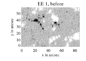
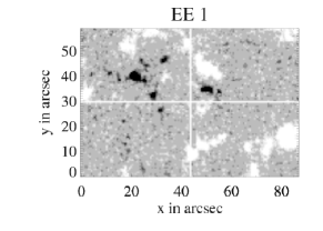
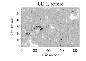
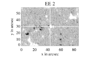
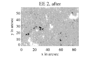
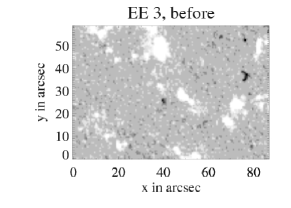
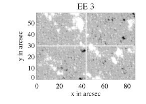
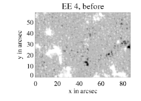
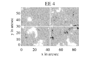
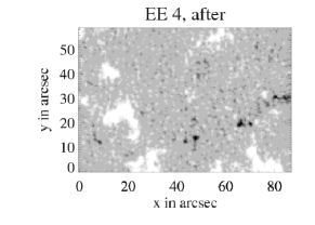
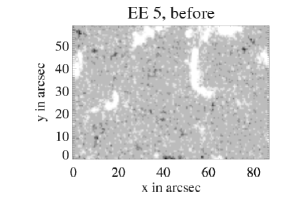
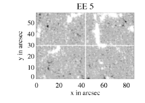
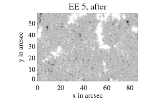
Figure 3: Examples of magnetic flux evolution at the location of an EE, images are saturated at $B=\pm$ 30 Mx cm^-2. Left: a magnetogram taken 30 min before the EE took place. Center: a magnetogram at the time of the EE, with the EE being located in the center of the FOV (indicated by the white cross). Right: a magnetogram taken 30 min after the EE. The 2 top rows show flux cancellation, the third row flux emergence, the fourth row complex flux changes and in the bottom row there are no flux changes.

Figure 3 presents several examples of magnetic flux changes observed at the locations of EEs. The images are saturated at $B=\pm$30 Mx cm^-2. In each example the left image is a magnetogram taken 30 min before the EE took place, the central image shows the distribution of magnetic flux at the time of the EE, which is located at the center of the FOV (as indicated by the white cross), and the right image is the magnetogram taken 30 min after the EE. Movies of these and several other events can be found at http://wwwsolar.nrl.navy.mil/$\sim$muglach/ee.html .

The following description of the magnetic flux evolution refers to the complete movies, where Figure 3 only shows snapshots for each case. An example of flux cancellation can be seen in the top row of Figure 3. Near the center of the FOV there is a large patch of white–polarity flux with a small piece of black–polarity flux next to it. Just to the north there is a large black–polarity patch with a small white–polarity area on its east side. In both places the minority polarity moves towards the larger magnetic patch and slowly disappears. Both areas of cancelling flux lie within our 6^′′ radius around the EE location.

The second row of Figure 3 shows another example of flux cancellation: again, a very small patch of one (black) polarity approaches a larger patch of the other (white) polarity and completely vanishes by the end of the 1h sequence.

The third row Figure 3 illustrates an example of flux emergence at the EE site. Although there is a bipole present near the center of the FOV at the beginning of the sequence, a second small bipole appears subsequently. The new bipole eventually becomes clearly visible in the right image at the end of the 1h period.

The fourth row shows complex flux changes: during the first half an hour a small bipole emerges, which cancels again in the second half an hour. Finally the bottom row is a typical example where we do not find any flux changes around the EE site.

Table 1 summarizes our results. Out of a total of 37 EEs we find that 14 (38%) show flux changes in a time interval of 1h around the time of the EE. We have 3 cases of flux emergence, 7 cases of flux cancellation and 4 complex cases with both emergence and cancellation taking place within our 6^′′ radius of the EE location. For 23 EEs (62%) we could not identify any significant flux changes. In the second line of Table 1 we show the distribution of flux changes at randomly selected locations in the SUMER scans. Only 4 (11%) of the random locations show flux changes similar to the ones we find at EE locations.

Visual inspection of the MDI Dopplergram sequences did not reveal any signatures we might expect in connection with the restructuring of the magnetic field.

4 Discussion

All of our SUMER observations were taken in very quiet regions. Comparing the observed FOV with EIT EUV images we find that the observations were taken in a coronal hole. Therefore, the observed MDI flux densities are very low. As can be seen from Fig. 2, EEs are usually located near, but not directly inside the bright network (although a couple of exceptions can be found). While the flux density of the network is between 100 Mx cm^-2 and several hundred Mx cm^-2, values of the cancelling/emerging flux are between 20 Mx cm^-2 and less than 100 Mx cm^-2. The sizes of the flux patches are also very small (a few arcsec): usually just small bipoles or one small unipolar patch of flux cancelling with a larger network fragment. The duration of the flux changes cannot be determined as our 1h time window generally includes only part of the process. Because we only see snapshots of EEs in our SUMER data, such an investigation would require continuous observations at a given location.

From Table 1 we can see that the number of EE sites with flux changes clearly exceeds the number of random locations that show flux changes. Therefore, we believe that the flux changes we find are not just accidental occurrences. The ratio of flux cancellation to flux emergence is 7:3. This is very close to the ratio of about 2:1 found by Webb et al. (1993) studying the correspondence between X–ray bright points and evolving magnetic features in the quiet Sun, and Harvey (1985) for He I dark points. As explained in our introduction X–ray bright points emit at higher temperatures, are larger and have longer lifetimes than EEs. The flux involved is also stronger than what we measure in EEs. Nevertheless, both studies give about the same ratio. Webb et al. also find several cases of both emerging and cancelling flux, corresponding to what we call complex. In summary, we find several similarities between our results and the results of Webb et al. with regard to their magnetic field data, although we do not consider EEs smaller versions of X–ray bright points. Webb et al. (1993) also found that there were many more flux cancellation sites than X–ray bright points. We can speculate that one of the reasons might be that, to produce X–ray bright points reconnection has to occur in the corona, while reconnection taking place in the TR will produce EEs. In case the reconnection happens in even lower layers, e.g., in the photosphere, we would still measure flux cancellation, but neither EEs nor X–ray bright points.

To properly interpret the MDI magnetograms we need to understand how the flux densities are derived. The quantity that an imaging magnetograph measures is the circular polarization or Stokes $V$. Based on the longitudinal Zeeman effect this Stokes $V$ signal is interpreted as originating from a magnetic field permeating the plasma that the spectral lines originates from (e.g., Stenflo 1994, Lites 2000). In a filtergraph Stokes $V$ is usually measured in the wing of a spectral line, where the polarization signal is largest. In case of MDI the polarization is measured at several wing locations (Scherrer et al. 1995). A number of assumptions are made in converting the resulting signal to a magnetic field. Only the component of the magnetic field vector ${\bf B}$ along the line–of–sight produces circular polarization (the component in the plane perpendicular to the line–of–sight produces linear polarization, Stokes $Q$ and $U$, which are not measured). If one observes at disk center and the direction of the magnetic field vector is radial, then the LOS component can be equal to the actual field strength. Whenever the inclination angle between the field vector ${\bf B}$ and the line–of–sight ($\gamma$) changes however, so will the measured polarization signal.

We would like to add that the assumption that the polarization signal is proportional to the magnetic field strength is valid only in the so–called weak field regime, that is when, the Zeeman splitting is small compared to the Doppler width of the spectral line. This regime depends on the spectral line and usually breaks down at high field strengths like in a sunspot.

Another parameter that influences Stokes $V$ is the magnetic filling factor (FF). If one assumes a simple two–component model of the magnetic field, then the pixel under consideration contains contributions from both a magnetized and an unmagnetized atmosphere. In the conversion of the MDI polarization signal it is assumed that the observed pixel is completely permeated with magnetic field of constant strength (FF=1). But a field that is e.g. twice as strong but only covers half the area of the spatial resolution element will give the same polarization signal. Since the filling factor cannot be determined with filtergrams, the quantity that MDI delivers is a line–of–sight magnetic flux density, not a field strength $|{\bf B}|$. From full Stokes polarimetry we know that only sunspot umbrae have FF$\approx$1. For the quiet Sun, one has to differentiate between the magnetic network and internetwork. Network (and plage regions) are known to consist of magnetic elements with field strengths of about 1500 G and sizes of around 100 km ($<$ 0.2^′′). Filling factors for these regions range from FF=0.05 in quiet network up to 0.24–0.40 in plage regions (e.g. Stenflo 1973, Muglach & Solanki 1992, Martínez Pillet et al. 1997, Bellot Rubio et al. 2000).

The topology of the internetwork field is controversial. Depending on the assumed model and the spectral lines used, fields with moderate field strength around several dozens to hundreds of G can be found, or again kG fields with very small filling factors (see e.g. recent works from Martínez González et al. 2006, 2008 and Socas–Navarro et al. 2008). New observations with the spectro-polarimeter onboard the Hinode satellite with higher sensitivity and no interference from atmospheric seeing will provide new input into this unresolved issue. First results on internetwork fields from Hinode can be found e.g. in Orozco Suárez et al. (2007), Lites et al. (2008) and de Wijn et al. (2008).

The MDI movies show fluctuations of small flux densities on very short temporal and spatial scales. These flux densities are above $B=\pm$ 9 Mx cm^-2, which is our one sigma noise level. Most of these fluctuations are probably caused by changes in inclination $\gamma$ due to the swaying of the field lines in the granular velocity field, perhaps in addition to changes in FF as the field lines are shuffled together by the granules. As these fluctuations take place all over the observed field, we think that they are unrelated to EEs, or one would find a lot more EEs along the slit. The flux changes we consider significant for EEs involve somewhat larger flux patches that are persistent over more than one granular lifetime. We think that due to these rather conservative criteria, we do not find flux changes for the majority of our EEs. In addition, the magnetic sensitivity and spatial resolution of MDI are very limited. We hope that future observations from ground and especially from space (e.g. from Hinode/SOT) will improve these statistics and contribute to our understanding of small-scale photospheric dynamics reflected in magnetograms.

Visual inspection of the Dopplergram sequences did not reveal any velocity signatures we would expect in connection with the restructuring of the magnetic field. If flux emergence is really connected to flux elements moving from subphotospheric layers upward into the photosphere and higher layers, eventually leading to reconnection with pre-existing flux in the TR, one would expect to see upflows in connection with flux emergence. Or if flux submerges as a consequence of flux cancellation, one would expect to see downflows at the location of the cancelling flux (under the assumption that the reconnected loop is actually pulled under the surface). After p–mode filtering the Doppler velocity field shows fluctuations of the order of $\pm$ 600 m ${\rm s^{-1}}$ due to granular and supergranular flows. Beyond these fluctuations, however, no clear signature of e.g. downflows can be found at flux cancellation sites. However, the MDI Dopplergram signal is dominated by the non-magnetic part of the atmosphere within the observed pixel, while the magnetic field covers probably only a small fraction of the area. A better way to investigate this question would be to measure Stokes $V$ profiles and search for velocity signatures in the Stokes $V$ zero-crossing (e.g. Muglach & Solanki 1992) which reflects Doppler shifts originating exclusively from the magnetic part of the atmosphere. Increasing the spatial resolution should also increase the likelyhood of detecting velocity signatures.

As mentioned in the Introduction Chae et al. (1998) also compared SUMER EEs with line–of–sight magnetograms taken at BBSO. They found that about 64% of their EEs occurred during magnetic flux cancellation, while they did not mention any flux emergence. Their result differs considerably from our statistics and hence deserves closer inspection. The SUMER spectra that they analysed were taken in a sit–and–stare mode of the spectrograph. Therefore, due to the lack of solar rotation compensation solar structures moved through the 1^′′ slit in about 420s. During the 4.5h of their observing run, SUMER covered a region of about 40^′′ from which they construct a spectroheliogram that is compared with the magnetograms. They explained their method of identifying EEs in the SUMER spectra, but did not provide information on how EEs were counted in their analysis. Their Figure 1 shows the recurrence of an EE in a sequence of exposures, but it is unclear whether this would be considered to be one or two EEs in their statistics. This lack of information complicates an actual comparison of the respective results. The magnetograph data in their Figure 2 suggests that there are just two locations of flux cancellation, but it is unclear how many EEs were actually assigned to them. In contrast, our SUMER data represent snapshots of the TR with no information about the evolution of the EEs, whose lifetimes are comparable with our exposure times and sizes similar to the step size of the scan.

Unlike Chae et al. (1998), we also find flux emergence and complex flux changes in connection with EEs. Therefore, we propose that what we see is a signature of reconnection related to a change in magnetic topology of the small–scale magnetic field of quiet sun regions. This is a more general concept than flux cancellation.

A number of modelling efforts have been reported, e.g. Karpen et al. (1998), Sarro et al. (1998), Roussev & Galsgaard (2002) and Chen & Priest (2006). Chen & Priest (2006) model EEs under the influence of 5 min p-mode oscillations, trying to reproduce the recurrence rate of 5 min reported by Ning et al. (2004). They do get a 5 min modulation in their synthetic TR line, but the modulation is present in the central component of the line whereas no enhanced line wings are present. Some of the simulations of Roussev & Galsgaard (2002) on the other hand reproduce the line wing enhancements of their TR lines very well (see e.g. their Figure 5), but also produce wing enhancements in the coronal line Ne VIII 770 Å, which are usually not observed (most of the EEs in our sample are observed in C IV 1548 Å and also include simultaneous observations of Ne VIII 770 Å ). One of the challenges for modelling seems to be the fact that EEs are observed in TR lines, but not in coronal lines. The reconnection scenario therefore has to produce appropriate acceleration of sufficient plasma (not just heating) at TR temperatures, without heating and accelerating the plasma to coronal temperatures. Up to now modelling efforts are still too simplified to allow a detailed comparison with observations. We hope that the results of our detailed study of the photospheric field evolution will provide valuable input into future models.

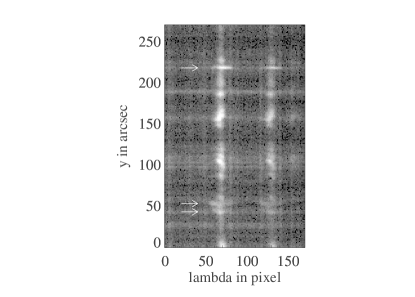
Figure 1: Example of C IV spectra at 1548 Å and 1550 Å (left), the white arrows point out the location of the EEs in this particular slit position. The line plots show the line profiles at the indicated arrow positions, the solid line represents the EE profile, the dashed line a profile averaged along the slit.

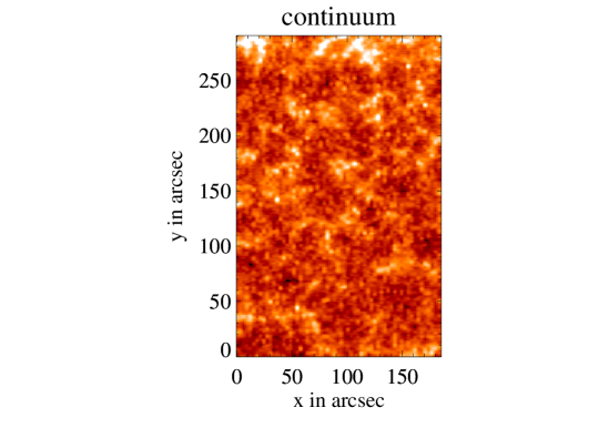
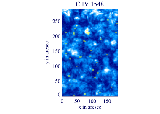
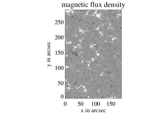
Figure 2: Example of a SUMER scan. Left: image of continuum intensity around 1535 Å. Center: the peak intensity of C IV 1548 Å. The yellow areas are locations of EEs, identified by strong wing enhancements in the C IV line. Right: magnetogram composed of a slice through the MDI 3-D data cube, following the SUMER scan.

Table 1: Magnetic flux changes observed during explosive events

		flux changes			no flux changes	total number
				all flux
	emergence	cancellation	complex	changes
explosive events	3	7	4	14/38%	23/62%	37
random locations	2	1	1	4/11%	33/89%	37

References

- Bellot Rubio et al. (2000) Bellot Rubio, L. R., Ruiz Cobo, B., & Collados, M. 2000, ApJ, 535, 489
- Bewsher et al. (2002) Bewsher, D., Parnell, C. E., & Harrison, R. A. 2002, Sol. Phys., 206, 21
- Bewsher et al. (2005) Bewsher, D., Innes, D. E., Parnell, C. E., & Brown, D. S. 2005, A&A, 432, 307
- Brković & Peter (2004) Brković, A., & Peter, H. 2004, A&A, 422, 709
- Brooks et al. (2004) Brooks, D. H., et al. 2004, ApJ, 602, 1051
- Brueckner & Bartoe (1983) Brueckner, G. E., & Bartoe, J.-D. F. 1983, ApJ, 272, 329
- Chae et al. (2000) Chae, J., Wang, H., Goode, P. R., Fludra, A., & Schühle, U. 2000, ApJ, 528, L119
- Chae et al. (1998) Chae, J., Wang, H., Lee, C.-Y., Goode, P. R., & Schuehle, U. 1998, ApJ, 497, L109
- Chen & Priest (2006) Chen, P. F., & Priest, E. R. 2006, Sol. Phys., 238, 313
- Dere (1994) Dere, K. P. 1994, Advances in Space Research, 14, 13
- Dere et al. (1984) Dere, K. P., Bartoe, J.-D. F., & Brueckner, G. E. 1984, ApJ, 281, 870
- Dere et al. (1991) Dere, K. P., Bartoe, J.-D. F., Brueckner, G. E., Ewing, J., & Lund, P. 1991, J. Geophys. Res., 96, 9399
- Dere & Martin (1994) Dere, K. P., & Martin, S. F. 1994, Proceedings of Kofu Symposium, 289
- Habbal (1992) Habbal, S. R. 1992, Annales de Geophysique, 10, 34
- Hagenaar (2001) Hagenaar, H. J. 2001, ApJ, 555, 448
- Harrison (1997) Harrison, R. A. 1997, Sol. Phys., 175, 467
- Harvey (1985) Harvey, K. L. 1985, Australian Journal of Physics, 38, 875
- Innes et al. (1997) Innes, D. E., Inhester, B., Axford, W. I., & Willhelm, K. 1997, Nature, 386, 811
- Lites (2000) Lites, B., 2000, Encyclopedia of Astronomy and Astrophysics
- Lites et al. (2008) Lites, B. W., et al. 2008, ApJ, 672, 1237
- Madjarska & Doyle (2003) Madjarska, M. S., & Doyle, J. G. 2003, A&A, 403, 731
- Madjarska et al. (2003) Madjarska, M. S., Doyle, J. G., Teriaca, L., & Banerjee, D. 2003, A&A, 398, 775
- Martínez González et al. (2008) Martínez González, M. J., Collados, M., Ruiz Cobo, B., & Beck, C. 2008, A&A, 477, 953
- Martínez González et al. (2006) Martínez González, M. J., Collados, M., & Ruiz Cobo, B. 2006, A&A, 456, 1159
- Martinez Pillet et al. (1997) Martínez Pillet, V., Lites, B. W., & Skumanich, A. 1997, ApJ, 474, 810
- Muglach & Solanki (1992) Muglach, K., & Solanki, S. K. 1992, A&A, 263, 301
- Ning et al. (2004) Ning, Z., Innes, D. E., & Solanki, S. K. 2004, A&A, 419, 1141
- Orozco Suárez et al. (2007) Orozco Suárez, D., et al. 2007, ApJ, 670, L61
- Parnell (2002) Parnell, C. E. 2002, MNRAS, 335, 389
- Pérez & Doyle (2000) Pérez, M. E., & Doyle, J. G. 2000, A&A, 360, 331
- Porter & Dere (1991) Porter, J. G., & Dere, K. P. 1991, ApJ, 370, 775
- Roussev & Galsgaard (2002) Roussev, I., & Galsgaard, K. 2002, A&A, 383, 697
- Sánchez Almeida et al. (2007) Sánchez Almeida, J., Teriaca, L., Sütterlin, P., Spadaro, D., Schühle, U., & Rutten, R. J. 2007, A&A, 475, 1101
- Scherrer et al. (1995) Scherrer, P. H., et al. 1995, Sol. Phys., 162, 129
- Settele et al. (2002) Settele, A., Carroll, T. A., Nickelt, I., & Norton, A. A. 2002, A&A, 386, 1123
- Sheeley & Golub (1979) Sheeley, N. R., Jr., & Golub, L. 1979, Sol. Phys., 63, 119
- Socas–Navarro et al. (2008) Socas–Navarro, H., et al. 2008, ApJ, 674, 596
- Stenflo (1994) Stenflo, J. O. 1994, Astrophysics and Space Science Library, 189,
- Stenflo (1973) Stenflo, J. O. 1973, Sol. Phys., 32, 41
- Tarbell et al. (2000) Tarbell, T. D., Ryutova, M., & Shine, R. 2000, Sol. Phys., 193, 195
- Teriaca et al. (2004) Teriaca, L., Banerjee, D., Falchi, A., Doyle, J. G., & Madjarska, M. S. 2004, A&A, 427, 1065
- Webb et al. (1993) Webb, D. F., Martin, S. F., Moses, D., & Harvey, J. W. 1993, Sol. Phys., 144, 15
- de Wijn et al. (2008) de Wijn, A. G., Lites, B. W., Berger, T. E., Frank, Z. A., Tarbell, T. D., & Ishikawa, R. 2008, ArXiv e-prints, 806, arXiv:0806.0345
- Wilhelm et al. (1995) Wilhelm, K., et al. 1995, Sol. Phys., 162, 189