Changes in the Distribution of Income Volatility

Abstract

Recent research has documented a significant rise in the volatility (e.g., expected squared change) of individual incomes in the U.S. since the 1970s.  Existing measures of this trend abstract from individual heterogeneity, effectively estimating an increase in average volatility.  We decompose this increase in average volatility and find that it is far from representative of the experience of most people: there has been no systematic rise in volatility for the vast majority of individuals.  The rise in average volatility has been driven almost entirely by a sharp rise in the income volatility of those expected to have the most volatile incomes, identified ex-ante by large income changes in the past.  We document that the self-employed and those who self-identify as risk-tolerant are much more likely to have such volatile incomes; these groups have experienced much larger increases in income volatility than the population at large.  These results color the policy implications one might draw from the rise in average volatility.  While the basic results are apparent from PSID summary statistics, providing a complete characterization of the dynamics of the volatility distribution is a methodological challenge.  We resolve these difficulties with a Markovian hierarchical Dirichlet process that builds on work from the non-parametric Bayesian statistics literature.

1 Introduction

A large literature argues that income volatility – the expectation of squared individual income changes – has increased substantially since the 1970s in the U.S., with further increases since the 1990s. To the degree that people are risk-averse and income volatility is taken as a proxy for risk, ceteris paribus such rising volatility may carry substantial welfare costs.  As a consequence, there has been a great deal of recent interest by politicians and journalists in this finding. (Gosselin2004; Scheiber2004; HouseHearings2007)

To date, research on income volatility trends has ignored individual heterogeneity, effectively estimating an increase in average volatility.  We decompose this increase in the average and find that it is far from representative of the experience of most people: there has been no systematic increase in volatility for the vast majority of individuals.  The increase has been driven almost entirely by a sharp increase in the income volatility of those with the most volatile incomes.  In turn, we find that these individuals with high – and increasing – volatility more likely to be self-employed and more likely to self-identify as risk-tolerant.

Our main finding is apparent in simple summary statistics from the PSID.  For example, divide the sample into cohorts, comparing the minority who experienced very large absolute one-year income changes in the past (e.g., four years ago) to those who did not.  Since volatility is persistent, those identified ex-ante by large past income changes naturally tend to have more volatile incomes today.  The income volatility of this group identified ex-ante as high-volatility has increased since the 1970s while the income volatility of others has remained roughly constant.  This divergence of sample moments identifies our key result.

Obviously, these findings could affect substantially the welfare and policy implications of the rise in average volatility.  The individuals whose volatility has increased – who we find are those with the most volatile incomes – may be those with the highest tolerance for risk or the best risk-sharing opportunities.  Such risk tolerance is apparent not only from the willingness of these individuals to undertake volatile incomes or self-employment in the first place, but also from their answers to survey questions.

While the basic results can be seen in summary statistics, providing a complete characterization of the dynamics of the volatility distribution is a methodological challenge.  We use a standard model for income dynamics that allows income to change in response to permanent and transitory shocks.  What is less standard is that we allow the variance of these shocks – our income volatility parameters – to be heterogeneous and time-varying.

We estimate a discrete non-parametric model in which volatility parameters are assumed to take one of L unique values, where the number L and the values themselves are determined by the data.  We add structure and get tractability with a variant on the Dirichlet process (DP) prior commonly used in Bayesian statistics.  The Markovian hierarchical DP prior model we develop accounts for the grouped nature of the data (by individual) as well as the time-dependency of successive observations within individuals.  Implicitly, we place a prior on the probability that an individual’s parameter values will change from one year to the next, on the number of unique parameter values an individual will hold over his lifetime, and on the number of unique parameter values found in the sample.

In Section 2, we discuss our data and the summary statistics that drive our results.  In Section 3, we present our statistical model including the income process (Section 3.1), the structure we place on heterogeneity and dynamics in volatility parameters (Section 3.2), and our estimation strategy (Section 3.3).  In Section 4, we show the results obtained by estimating our model on the data.  Increases in the average volatility parameter are due to increases in volatility among those with the most volatile incomes (Section 4.2).  We find that the increase in volatility has been greatest among the self-employed and those who self-identify as risk-tolerant (Section 4.5), and that these groups are disproportionately likely to have the most volatile incomes (Section 4.4).  Increases in risk are present throughout the age distribution, education distribution, and income distribution (Section 4.5).  Section 5 concludes with a discussion of welfare implications.

2 Data and summary statistics

2.1 Data and variable construction

Data are drawn from the core sample of the Panel Study of Income Dynamics (PSID).  The PSID was designed as a nationally representative panel of U.S. households.  It tracked families annually from 1968 to 1997 and in odd-numbered years thereafter; this paper uses data through 2005.  The PSID includes data on education, income, hours worked, employment status, age, and population weights to capture differential fertility and attrition.   In this paper, we limit the analysis to men age 22 to 60; we use annual labor income as the measure of income.  Table 1 presents summary statistics from these data.

Table 1: Summary Statistics

	mean	st. dev.	min	max
year	$1986.3$	$10.0$	$1968$	$2005$
age (years)	$~{}40.0~{}$	$~{}10.5~{}$	$22$	$60$
education (years)	$~{}13.1~{}$	$~{}2.9~{}$	$0$	$17$
# of observations/person	$17.2$	$9.0$	$1$	$34$
married (1 if yes, 0 if no)	$~{}0.80~{}$	.	.	.
black (1 if yes, 0 if no)	$0.05$	.	.	.
annual income (2005 $s)	$\$50,553$	$\$57,506$	$0$	$\$3,714,946$
annual income ($s)	$\$29,277$	$\$46,818$	$0$	$\$3,500,000$
family size	$3.1$	$1.5$	$1$	$14$

This table summarizes data from 52,181 observations on 3,041 male household heads.

We want to ensure that changes in income are not driven by changes in the top-code (the maximum value for income entered that can be entered in the PSID).  The lowest top code for income was $99,999 in 1982 ($202,281 in 2005 dollars), after which the top-code rises to $9,999,999.  So that top-codes will be standardized in real terms, this minimum top-code is imposed on all years in real terms, so the top-code is $99,999 in 1982 and $202,281 in 2005.  Since our income process in Section 3.1 does not model unemployment explicitly, we need to ensure that results for the log of income are not dominated by small changes in the level of income near zero (which will imply huge or infinite changes in the log of income).  To address this concern, we replace income values that are very small or zero with a non-trivial lower bound.  We choose as this lower-bound the income that would be earned from a half-time job (1,000 hours per year) at the real equivalent of the 2005 federal minimum wage ($5.15 per hour).  This imposes a bottom-code of $5,150 in 2005 and $2,546 in 1982.  Note that the difference in log income between the top- and bottom-code is constant over time, so that differences over time in the prevalence of predictably extreme income changes cannot be driven by changes in the possible range of income changes.  The vast majority of the values below this bound are exactly zero.  This bound allows us to exploit transitions into and out of the labor force.  At the same time, the bound prevents economically unimportant changes that are small in levels but large and negative in logs from dominating the results.  Results are robust to other values for this lower bound, such as the income from full-time work (2,000 hours per year) at the 2005 minimum wage (in real terms).

Table 2: Distribution of Income, Excess Log Income, and Income Changes for Men

	Real Income		Excess Income
	Level		Level	One-Year	Five-Year
$\begin{array}[]{c}\mathrm{One-Year}\\ \mathrm{Change}\end{array}$	$\begin{array}[]{c}\mathrm{Five-Year}\\ \mathrm{Change}\end{array}$
Mean	$50,553 ($48,867)		0	0.0017	0.0043
St. Dev.	$57,506 ($34,943)		0.7307	0.4870	0.6863
Observations	52,181		52,181	43,261	34,972
Minimum	$0 ($5,150)		-2.9325	-3.6877	-3.8361
5th Percentile	$668 ($5,150)		-1.6283	-0.7323	-1.3046
25th Percentile	$26,174		-0.2964	-0.1089	-0.2126
50th Percentile	$42,887		0.1246	0.0134	0.0653
75th Percentile	$62,012		0.4601	0.1442	0.3072
95th Percentile	$113,500		0.9757	0.6673	0.9764
Maximum	$3,714,946 ($202,381)		2.6435	3.5862	4.0678

Table 2 describes the distribution of labor income for men in the PSID over the period from 1968 to 2005.  See Section 2 for a detailed description of the income variable and the top- and bottom-coding procedure. Column 1 shows the distribution of real annual income for men (in 2005 dollars).  The numbers in parentheses are the values with top- and bottom-coding restrictions.  Column 2 shows the distribution of “excess” log income, the residual from the regression of log labor income (with top- and bottom-code adjustments) on the covariates enumerated in Section 2.  Column 3 presents the distribution of one-year changes in excess log income.  Column 4 repeats the results for column 3, but presents five-year changes instead of one-year changes.

In this paper, we model the evolution of “excess” log income.  This is taken as the residual from a regression to predict the natural log of labor income (top- and bottom-coded as described).  The regression is weighted by the PSID-provided sample weights, with the weights normalized so that the average weight in each year is the same.  We use as regressors: a cubic in age for each level of educational attainment (none, elementary, junior high, some high school, high school, some college, college, graduate school); the presence and number of infants, young children, and older children in the household; the total number of family members in the household, and dummy variables for each calendar year.  Including calendar year dummy variables eliminates the need to convert nominal income to real income explicitly.  While this step is standard in the income process literature, it is not necessary to obtain our results.  The results to follow are qualitatively the same and quantitatively similar when we use log income in lieu of excess log income.

Table 2 presents data on the distribution of real annual income in column 1 (imposing top- and bottom-code restrictions in parentheses). While the mean real income is nearly identical with and without top- and bottom-code restrictions ($50,553 versus $48,867), these restrictions on extreme values reduce the standard deviation of real income from $57,506 to $34,943.  Column 2 shows the distribution of “excess” log income.  Since excess log income is the residual from a regression, its mean is zero.  The inter-quartile range of excess log income is $-0.30$ to $0.46$.

Column 3 presents the distribution of one-year changes in excess log income.  Naturally, the mean of one-year changes is close to zero.  The inter-quartile range of one-year changes is $-0.11$ to $0.14$; excess income does not change more than $11$ to $14$ percent from year to year for most individuals.  However, there are extreme changes in income, so the standard deviation of changes to log income ($0.49$) is far great than the inter-quartile range.  This implies either that changes to income have fat tails (so that everyone faces a small probability of an extreme income change), or alternatively that there is heterogeneity in volatility (so that a few people face a non-trivial probability of an extreme income change).  Unless a model is identified from parametric assumptions, these are observationally equivalent in a cross-section of income changes.  However, heterogeneity and fat tails have different implications for the time-series of volatility, and we exploit these in the paper.

Column 4 repeats the results from column 3, but presents five-year excess log income changes instead of one-year changes.  These long-term changes have only slightly higher standard deviations than the one-year change, $0.69$ vs. $0.49$, suggesting some mean-reversion in income.   AbowdCard89 show that while one-year income changes are highly negatively correlated at one-year lags, there is no evidence of autocorrelated income changes at lags greater than two years.

2.2 Volatility summary statistics

Table 3: Income Volatility Sample Moments

	Permanent Variance				Squared Change
	Mean	Median	95${}^{\mathrm{th}}\%$		Mean	Median	95${}^{\mathrm{th}}\%$
Average	0.1091	0.0099	0.8264		0.3561	0.0314	2.0042
% Change	49$\%$	15$\%$	92$\%$		110$\%$	19$\%$	143$\%$
1970-2003
Slope	0.0015	0.0000	0.0205		0.0106	0.0002	0.0775
(t-stat)	(4.11)	(0.52)	(8.76)		(11.96)	(1.26)	(11.18)
1970	.	.	.		0.1555	0.0210	0.7709
1971	.	.	.		0.1823	0.0229	0.8004
1972	0.0665	0.0059	0.4003		0.2142	0.0277	1.1276
1973	0.0786	0.0048	0.4423		0.2296	0.0269	1.1500
1974	0.0792	0.0054	0.5090		0.2324	0.0264	1.1059
1975	0.0986	0.0129	0.6243		0.2496	0.0380	1.2286
1976	0.0997	0.0179	0.6749		0.3124	0.0498	1.6006
1977	0.0933	0.0095	0.7058		0.2983	0.0316	1.8058
1978	0.0706	0.0062	0.5958		0.2751	0.0296	1.3344
1979	0.0838	0.0061	0.6415		0.2931	0.0269	1.6711
1980	0.1388	0.0115	0.9270		0.2811	0.0292	1.4495
1981	0.1159	0.0123	0.8844		0.2932	0.0296	1.5200
1982	0.1004	0.0150	0.7256		0.2514	0.0305	1.2840
1983	0.0859	0.0150	0.6630		0.2912	0.0330	1.5820
1984	0.1220	0.0126	0.8786		0.3185	0.0331	1.8609
1985	0.1109	0.0118	0.7869		0.3283	0.0370	1.7499
1986	0.1002	0.0110	0.6905		0.3089	0.0358	1.5483
1987	0.1089	0.0093	0.7739		0.3015	0.0295	1.6058
1988	0.1224	0.0087	0.7969		0.3121	0.0300	1.6476
1989	0.1161	0.0077	0.8171		0.3278	0.0276	1.8996
1990	0.1174	0.0091	0.7770		0.2998	0.0261	1.5937
1991	0.1312	0.0121	0.9905		0.3523	0.0309	1.8485
1992	0.1013	0.0111	0.9119		0.3168	0.0295	1.7572
1993	0.1272	0.0112	1.0935		0.4166	0.0333	2.3561
1994	0.1083	0.0104	0.9270		0.4479	0.0347	2.6530
1995	0.1346	0.0077	1.1290		0.4914	0.0333	3.3055
1996	.	.	.		0.4768	0.0264	3.1923
1997	0.0898	0.0074	0.8660		0.4671	0.0282	2.9644
1999	0.1142	0.0080	0.9632		0.4539	0.0317	2.7189
2001	0.1190	0.0073	1.1174		0.4463	0.0271	2.9567
2003	0.1487	0.0182	1.2951		0.6348	0.0574	3.9098

The year $t$ permanent variance is the product of two-year changes in excess log income (from $t-2$ to $t$) and the six-year changes that span them (from $t-4$ to $t+2$).  The year $t$ squared change is from $t-2$ to $t$.  The first row shows full sample moments.  The second row shows the percent change over the sample, calculated as the coefficient of a weighted OLS regression of year-specific sample moments on a time trend, multiplied by the number of years (2005-1968) and divided by the full sample moment.  The coefficient and t-statistic are shown below.

Table 3 shows the evolution of volatility sample moments over time.  The first three columns show the variance of permanent income changes.  The final three columns present two-year squared changes in excess log income, a raw measure of income volatility. Note that while the mean size of an income change (columns 1 and 4, Table 3) has increased over time, the median (columns 2 and 5) has not.  This divergence can be explained by an increase in the magnitude of large unlikely income changes (columns 3 and 6).  While not framed in this way, these features of the data have been identified in previous research, including Dynanetal2007.

Table 4: Income Volatility Sample Moments by Past Volatility

	Permanent Variance			Squared Change
Moment	Mean			Mean
Past Variance	Low	High		Low	High
Average	0.0820	0.3845		0.2675	0.6879
$\%$ Difference	92$\%$			54$\%$
Slope	0.00083	0.020		0.0080	0.026
(t-stat)	(1.29)	(4.36)		(8.67)	(6.61)
1974	.	.		.	.
1975	.	.		.	.
1976	0.1015	0.2895		0.2265	0.5304
1977	0.0935	0.3260		0.2164	0.5917
1978	0.0374	0.1955		0.1540	0.3231
1979	0.0491	0.3720		0.2017	0.4381
1980	0.0786	0.3663		0.1972	0.5860
1981	0.0668	0.2558		0.1780	0.5981
1982	0.0608	0.2214		0.1964	0.5569
1983	0.0676	0.0927		0.1806	0.5065
1984	0.1285	0.3449		0.2426	0.4804
1985	0.0757	0.2262		0.2708	0.4550
1986	0.1178	0.0190		0.2210	0.6276
1987	0.0753	0.3392		0.2532	0.4401
1988	0.0600	0.2691		0.2381	0.6474
1989	0.0701	0.3087		0.2430	0.6448
1990	0.0964	0.4907		0.2143	0.3365
1991	0.1108	0.4253		0.2846	0.8574
1992	0.0783	0.3356		0.2498	0.5450
1993	0.0889	0.6556		0.2990	0.8766
1994	0.0569	0.2607		0.3339	0.7283
1995	0.1105	0.5464		0.3327	0.8622
1996	.	.		0.3590	0.8988
1997	0.0428	0.9663		0.3375	0.8572
1999	0.0865	0.6554		0.3309	1.2439
2001	0.1049	0.4295		0.3115	1.0118
2003	0.1101	0.8355		0.4460	1.2074

The year $t$ permanent variance is the product of two-year changes in excess log income (from $t-2$ to $t$) and the six-year changes that span them (from $t-4$ to $t+2$).  The first and third columns show sample means for the cohort of individuals whose permanent variance and squared change, respectively, were below median in the year four years prior.  The second and fourth columns show the same, but for the cohorts with past values above the 95^th percentile four years prior.  The first row shows full sample moments.  The third and fourth rows present the coefficient and t-statistic from a weighted OLS regression of year-specific sample means on a time trend.  The difference in these two coefficients, divided by their average, is the $\%$ difference in the second row.  Year-by-year means are shown below.

Figure 1: Comparing Sample Variances for Those With and Without Large Past Income Changes

Permanent Variance	Squared Change

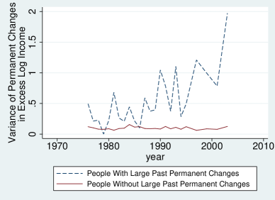
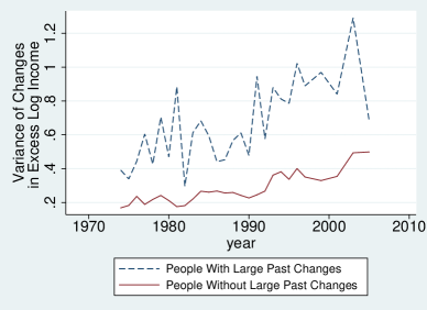
Following MeghirPistaferri2004, the sample permanent variance is calculated as the product of two-year changes in excess log incomes (between years t and t-2) and the six-year changes that span them (between years t+2 and t-4).  The sample transitory variance is calculated as the square of two-year changes in excess log income.  Individuals are defined as low past variances when their sample variance (permanent or transitory, respectively) four years ago is below median; individuals are defined as high past variance when their sample variance four years ago is above the 95^th percentile.  Weighted averages for these groups are presented in each year for which data is available for permanent variance (left panel) and transitory variance (right panel).

Table 4 and Figure 1 show the evolution of volatility sample moments separately for those who are ex-ante likely or unlikely to have volatile incomes.  The left panel of Table 4 presents the sample mean of the permanent variance; the right panel presents the mean two-year squared excess log income change.  For each year, the sample is split into two groups (below median or above 95^th percentile) based on the absolute magnitude of permanent (left panel) or squared (right panel) changes four years prior.  Unsurprisingly, individuals with large past income changes tend to have larger subsequent income changes.  The tendency to have large income changes is persistent, which indicates that some individuals have ex-ante more volatile incomes than others.

If (as we argue) volatility is increasing for high-volatility individuals but not for low-volatility individuals, then the gap in the sample variance between those with and without large past income changes should be increasing over time.  This divergence over time in volatility between past low- and high-volatility cohorts is clear in both Table 4 and Figure 1.  The magnitude of income changes has been increasing more for those with large past income changes (who are more likely to be inherently high-volatility) than for those without such large past income changes (who are not).  This is particularly apparent for the permanent variance; for the transitory variance, the finding is obscured slightly by the jump in volatility for everyone in the early- to mid-nineties (when the PSID changed to an automated data collection system which may have led to increased measurement error in income).  This divergence illustrates the key stylized fact developed in this paper: the increase in income volatility can be attributed to an increase in volatility among those with the most volatile incomes, identified ex-ante by large past income changes.

3 Statistical model

3.1 Income process

Here, we present a standard process for excess log income for individual $i$ at time $t$ (following CarrollSamwick97; MeghirPistaferri2004, and many others):

$$y_{i,t} = p_{i,t}+\xi_{i,t}+e_{i,t}$$ (1)

$$p_{i,t} = p_{i,0}+\sum\limits_{k=1}^{t-q_{\omega}}\omega_{i,k}+\sum\limits_{k=t-q_{\omega}+1}^{t}\phi_{\omega,t-k}\omega_{i,k}\mathrm{.}$$

$$\xi_{i,t} = \sum\limits_{k=t-q_{\varepsilon}+1}^{t}\phi_{\varepsilon,t-k}\varepsilon_{i,k}$$

Excess log income ($y_{i,t}$) is the sum of permanent income ($p_{i,t}$), transitory income ($\xi_{i,t}$), and measurement error ($e_{i,t}$).   The permanent shock, transitory shock, and measurement error are assumed to be normally distributed with mean zero as well as independent of one another, over time and across individuals.  Permanent income is initial income ($p_{i,0}$) plus the weighted sum of past permanent shocks ($\omega_{i,k},0<k\leq t$) with variance $\sigma^{2}_{\omega,i,t}\equiv E\left[\omega_{i,t}^{2}\right]$.  Transitory income is the weighted sum of recent transitory shocks ($\varepsilon_{i,k}$) with variance $\sigma^{2}_{\varepsilon,i,t}\equiv E\left[\varepsilon_{i,t}^{2}\right]$.  We refer to $\sigma^{2}_{i,t}\equiv(\sigma^{2}_{\varepsilon,i,t},\sigma^{2}_{\omega,i,t})$ jointly as the volatility parameters.  These will be allowed to differ between individuals to accommodate heterogeneity, and to evolve over time.  This accommodates not just an evolving distribution of volatility parameters, but also systematic changes over the life-cycle in volatility paramters, as suggested by ShinSolon2008.  Subcripts for $i$ and $t$ indicate that volatility parameters may differ across individuals and over time, as discussed in Section 3.2.  “Noise variance”refers to the variance of measurement error, $\gamma^{2}\equiv E\left[e_{i,t}^{2}\right]$.  This measurement error could be subsumed into transitory income; it is kept separate only to accommodate our estimation strategy.

Here, permanent shocks come into effect over $q_{\omega}$ periods, and transitory shocks fade completely after $q_{\varepsilon}$ periods.  As an example of our notation, $\phi_{\omega,2}$ denotes the weight placed on a permanent shock from two periods ago, $\omega_{i,t-2}$, in current excess log income; $\phi_{\varepsilon,2}$ denotes the weight placed on a transitory shock from two periods ago, $\varepsilon_{i,t-2}$, in current excess log income.  While we use the word “shock” for parsimony, these innovations to income may be predictable to the individual, even if they look like shocks in the data.  Without loss of generality, we impose the constraint that the weights placed on transitory shocks sum to one ($\sum_{k}\phi_{\varepsilon,k}=1$).

3.2 Heterogeneity and dynamics

We characterize the dynamics of volatility parameters, $\sigma^{2}_{i,t}$, using a discrete non-parametric approach.  In a discrete non-parametric model, the variable of interest – here, the pair $\sigma^{2}_{i,t}\equiv(\sigma^{2}_{\varepsilon,i,t},\sigma^{2}_{\omega,i,t})$ – can take one of $L$ possible values, $\{\sigma^{2}_{l}\}_{l=1}^{L}$ (where $L$ and $\{\sigma^{2}_{l}\}_{l=1}^{L}$ for any given sample are determined by the data).  The probability that $\sigma^{2}_{i,t}$ takes a given value is a function of a) the distribution of values in the population, $\{\Pi_{l}\}$, where $\Pi_{l}$ is the proportion of the population whose parameter values are equal to $\sigma^{2}_{l}$, b) the distribution of values for each individual $i$, $\{\Pi_{l_{i}}\}$, where $\Pi_{l_{i}}$ is the proportion of individual $i$’s observations with parameter values are equal to $\sigma^{2}_{l}$,, and c) the number of consecutive years $Q_{i,t}$ with the most recent value.  In other words, $\sigma^{2}_{i,t}$ has a given probability of changing from one year to the next; when it changes, it changes to a value drawn from the individual’s distribution, $\{\Pi_{l_{i}}\}$, which in turn consists of values drawn from the population distribution, $\{\Pi_{l}\}$.

We add structure and get tractability by adding a prior commonly used in Bayesian analysis of such discrete non-parametric problems: the Dirichlet process (DP) prior.  In a standard DP model, there is a “tuning parameter”, $\Theta$, which implicitly places a prior on the total number of unique parameter values in the sample, $L$.  $\Theta$ is defined more formally in Section 3.3.  We set $\Theta=1$, though our inference is not sensitive to this choice.  In a hierarchical DP (HDP) model (recently developed by TehJorBea06), the usual DP model is extended so by adding a second tuning parameter, $\Theta_{i}$, which implicitly places a prior on the total number of unique parameter values for any given individual, $L_{i}$; we set $\Theta_{i}=1$.

We extend this approach further to address panel data by including a Markovian structure on the hierarchical DP, giving us a Markovian hierarchical DP (MHDP) model.  In our Markovian approach, the prior probability that the parameter is unchanged from the previous period depends on the number of consecutive years with that value, $Q_{i,t}$.  We add a third tuning parameter, $\theta$, to place a prior on the probability of changing the parameter value, $p\left(\sigma^{2}_{i,t}=\sigma^{2}_{i,t-1}\ |i,t\right)=Q_{i,t}/(\theta+Q_{i,t})$; we set $\theta=1$.  In the MHDP model, our prior parameters can then be characterized with the triple $\boldsymbol{\Theta}\equiv\{\Theta,\Theta_{i},\theta\}=\{1,1,1\}$.

Given our research question, a key advantage of this set-up is that it does not restrict the shape (or the evolution of the shape) of the cross-sectional volatility distribution.  We view our discrete non-parametric model and the structure placed on it by our MHDP prior as providing a sensible middle ground between tractability and flexibility.

3.3 Estimation

We estimate the income process from Section 3.1 on annual data from the PSID (detailed in Section 2) for excess log income.  When data are missing, mostly because no data was collected by the PSID in even-numbered years following 1997, we impute bootstrapped guesses of income.  These bootstrapped values add no additional information; they merely accommodate our estimation strategy in a setting with missing data in a way that is intended to minimize the possible impact on our results.  Here, we outline an approach for combining the prior from Section 3.2 with data on excess log income, $\boldsymbol{y}$, to form a posterior on the distribution of volatility parameters, $\boldsymbol{\sigma^{2}}$.  Further details and an algorithm for implementation are provided in the appendix.

Consider the problem of estimating $\sigma^{2}_{i,t}$, the volatility parameters for person $i$ in year $t$, if all other parameters $\boldsymbol{\sigma^{2}_{-(i,t)}}$ (and $\boldsymbol{\phi}$) were known.  The decision tree for estimation is shown in Figure 2 and described here, both with references to relevant equations in the appendix.

1. $\sigma^{2}_{i,t}$ can remain unchanged from last year ($\sigma^{2}_{i,t}=\sigma^{2}_{i,t-1}$, eq: LABEL:eq:_prevchoice1) or can change ($\sigma^{2}_{i,t}\neq\sigma^{2}_{i,t-1}$, eq: LABEL:eq:_prevchoice2).  If $\sigma^{2}_{i,t}$ changes;

2. $\sigma^{2}_{i,t}$ can change to a value from the set of other values for that individual ($\sigma^{2}_{i,t}\in\boldsymbol{\sigma^{2}_{i,-t}}$ and $\sigma^{2}_{i,t}\neq\sigma^{2}_{i,t-1}$, eq: LABEL:eq:_personchoice1) or can take on a value new to the individual ($\sigma^{2}_{i,t}\notin\boldsymbol{\sigma^{2}_{i,-t}}$, eq: LABEL:eq:_personchoice2).  If $\sigma^{2}_{i,t}$ takes on a value new to the individual;

3. $\sigma^{2}_{i,t}$ can be a value held by other individuals ($\sigma^{2}_{i,t}\in\boldsymbol{\sigma^{2}_{-(i,t)}}$ and $\sigma^{2}_{i,t}\notin\boldsymbol{\sigma^{2}_{i,-t}}$, eq: LABEL:eq:_popchoice1) or can be a new value not shared with other individuals ($\sigma^{2}_{i,t}\notin\boldsymbol{\sigma^{2}_{-(i,t)}}$, eq: LABEL:eq:_popchoice2).

The probability that $\sigma^{2}_{i,t}$ takes a given value is a function of a) the likelihood of generating estimated shocks $(\omega_{i,t},\varepsilon_{i,t})$ given $\sigma^{2}_{i,t}$ and b) the prior probability of $\sigma^{2}_{i,t}$.

The prior probability that the parameter remains unchanged in Level 1 ($\sigma^{2}_{i,t}=\sigma^{2}_{i,t-1}$) is proportional to $Q_{i,t}$; the prior probability that the parameter changes is proportional to $\theta$.  If the parameter changes in Level 1 ($\sigma^{2}_{i,t}\neq\sigma^{2}_{i,t-1}$), the prior probability that $\sigma^{2}_{i,t}$ changes to a value held by that individual in another year in Level 2 is proportional to the number of times that value occurs in other years for that individual; the prior probability that $\sigma^{2}_{i,t}$ changes to a new value not seen for that individual in another year is proportional to $\Theta_{i}$.  If the parameter changes to a new value not seen for that individual in another year in Level 2, the prior probability that $\sigma^{2}_{i,t}$ changes to one of the other population values in Level 3 is proportional to the number of times that value occurs within the population; the prior probability that $\sigma^{2}_{i,t}$ changes to a new value not seen elsewhere in the population is proportional to $\Theta$.

A detailed outline of this estimation algorithm is given in the appendix.  The appendix shows this compound prior algebraically, and also shows how it is combined with the data to produce a posterior for $\sigma^{2}_{i,t}$.  We proceed iteratively through all $t$ within an individual and all $i$ across individuals.  This entire scheme for choosing volatility values $\boldsymbol{\sigma^{2}}$ is nested within a larger Gibbs sampling algorithm (GemGem84).  This Markov Chain Monte Carlo (MCMC) approach simultaneously estimates the other parameters of our model, namely shocks ($\boldsymbol{\omega},\boldsymbol{\varepsilon}$) and income coefficients ($\boldsymbol{\phi},\gamma^{2}$).

Figure 2: Model Hierarchy

4 Results

Table 5: Basic Model Results

Distribution of Variance Parameters

	$\begin{array}[]{c}\mathrm{Permanent}\\ \mathrm{Variance}\end{array}$	$\begin{array}[]{c}\mathrm{Transitory}\\ \mathrm{Variance}\end{array}$
Mean	0.0713	0.2771
St. Dev.	0.4685	1.0471
N	67,725	67,725
1st $\%$	0.0200	0.0499
5th $\%$	0.0250	0.0506
10th $\%$	0.0301	0.0510
25th $\%$	0.0313	0.0518
50th $\%$	0.0321	0.0530
75th $\%$	0.0331	0.0572
90th $\%$	0.0356	0.2452
95th $\%$	0.0498	1.2187
99th $\%$	0.8909	5.5030

Distribution of posterior means of $\boldsymbol{\sigma^{2}}$

Shocks’ Rate of Entry/Exit

lag	$\phi_{\omega,k}$	$\phi_{\varepsilon,k}$
$k=0$	0.381	0.784
	(0.088)	(0.029)
$k=1$	0.865	0.180
	(0.072)	(0.025)
$k=2$	0.951	0.037
	(0.064)	(0.017)

$\phi_{\omega,k}$: impact of permanent shock
   from $k$ periods ago
$\phi_{\varepsilon,k}$: impact of transitory shock
   from $k$ periods ago
Standard errors in parentheses.

The left panel presents the posterior mean estimates of the volatility parameters, $\boldsymbol{\sigma^{2}}$.  The distributions presented here consider all years and all individuals together.  The right panel of this table present $\boldsymbol{\phi}$, the mapping of shocks to income changes.

Figure 3: Distribution of Permanent and Transitory Variance

Permanent Variance	Transitory Variance

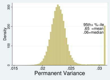
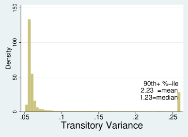
This figure presents the distribution of $\boldsymbol{\sigma^{2}_{\varepsilon}}$ and $\boldsymbol{\sigma^{2}_{\omega}}$.  These are the distribution of posterior means estimated from the data, as presented numerically in Table 5.  These posteriors of the permanent variance and transitory variance are calculated for each individual in each year, as described in Section 3.3.  The distributions presented here show all years and individuals together.  Values are truncated at the 95^th percentile for the permanent variance and at the 90th percentile for the transitory variance.  Mean and median of the truncated part of each distribution is given.

Here, we present the model parameters estimated using the methods from Section 3.3.  The chief object of interest is the evolution of the cross-sectional distribution of volatility parameters, $\boldsymbol{\sigma^{2}_{t}}$, over time.  These are shown in Section 4.2.  We begin with more basic results.  In subsection 4.1, we present estimates of the homogeneous parameters $\boldsymbol{\phi}$ that map shocks to income changes and the unconditional distribution of volatility parameters, $\boldsymbol{\sigma^{2}}$.  In Section 4.3, we rule out alternative explanations.  In Sections 4.4 and 4.5, we map these volatility parameter estimates to individuals’ demographic or risk attributes.

4.1 Basic results

Table 5 presents the basic parameter estimates obtained from fitting our model to the PSID income data described in Section 3.3.  The left panel shows the distribution of risk in the population, $\boldsymbol{\sigma^{2}_{\varepsilon}}$ and $\boldsymbol{\sigma^{2}_{\omega}}$.  Formally, we present the distribution of posterior means of permanent and transitory variance parameters.  The right panel show the mapping from shocks to income changes, $\boldsymbol{\phi}$, which we constrained to be constant over time and across individuals.

Figure 4: Impulse Response Function for Permanent and Transitory Shocks

Permanent Shock	Transitory Shock

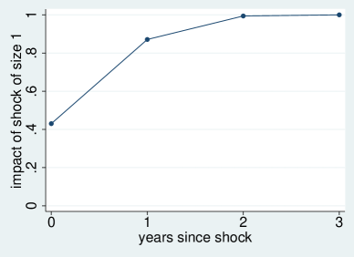
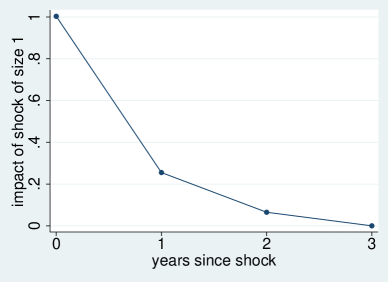
This figure presents an estimated impulse response function for a permanent (left panel) and transitory (right panel) shock.

Note the extreme skew and fat tails (kurtosis) in the distribution of volatility parameters, $\boldsymbol{\sigma^{2}}$, shown in the left panel of Table 5).  While medians are modest, means far exceed medians.  At the median, transitory shocks have a standard deviation of approximately 23% annually; permanent shocks have a standard deviation of just under 18% annually.  However, the highest volatility observations imply shocks with standard deviations well above 100% annually.  Figure 3 plots these skewed and fat-tailed distributions by truncating the right tail.

As shown in the right panel of Table 5, permanent shocks enter in quickly ($\phi_{\omega,k}$ are close to one) while transitory shocks damp out quickly ($\phi_{\varepsilon,k}$ fall to zero).  The impact of a shock on the evolution of income is presented in Figure 4.  These present impulse response functions for a permanent (left panel) and transitory (right panel) shock.  Shocks were calibrated as a one standard-deviation shock for an individual with volatility parameters at the estimated means (pulled from Table 5).

4.2 Evolution of the volatility distribution

Table 6: Year-by-Year Income Volatility Parameters

	Permanent Variance, $\sigma^{2}_{\omega}$				Transitory Variance, $\sigma_{\varepsilon}^{2}$
	Mean	Median	95${}^{\mathrm{th}}\%$		Mean	Median	95${}^{\mathrm{th}}\%$
Average	0.0713	0.0321	0.0498		0.2771	0.0530	1.2186
% Change	73$\%$	0$\%$	71$\%$		99$\%$	1$\%$	154$\%$
Slope	0.0014	0.0000	0.0010		0.0074	0.0000	0.0508
(t-stat)	(6.84)	(3.78)	(6.31)		(7.02)	(9.37)	(6.25)
1970	0.0573	0.0321	0.0424		0.1568	0.0526	0.4498
1971	0.0502	0.0321	0.0406		0.1901	0.0526	0.6419
1972	0.0411	0.0320	0.0374		0.1909	0.0527	0.7775
1973	0.0550	0.0321	0.0389		0.2027	0.0528	0.7997
1974	0.0481	0.0322	0.0437		0.1848	0.0528	0.5520
1975	0.0547	0.0321	0.0397		0.1923	0.0530	0.7597
1976	0.0663	0.0321	0.0464		0.2746	0.0529	1.3527
1977	0.0540	0.0321	0.0409		0.2424	0.0529	1.1020
1978	0.0557	0.0321	0.0411		0.1865	0.0529	0.6785
1979	0.0738	0.0321	0.0432		0.2226	0.0528	1.0134
1980	0.0748	0.0321	0.0452		0.2012	0.0529	0.7139
1981	0.0651	0.0321	0.0504		0.1986	0.0529	0.7762
1982	0.0594	0.0321	0.0502		0.2055	0.0529	0.8885
1983	0.0744	0.0321	0.0457		0.2550	0.0531	1.2691
1984	0.0660	0.0321	0.0503		0.2307	0.0531	0.9686
1985	0.0593	0.0321	0.0477		0.2260	0.0530	1.0063
1986	0.0672	0.0321	0.0441		0.2557	0.0529	1.1042
1987	0.0679	0.0321	0.0477		0.2448	0.0530	1.1468
1988	0.0714	0.0321	0.0467		0.2286	0.0531	0.9494
1989	0.0629	0.0321	0.0490		0.2462	0.0529	1.3182
1990	0.0801	0.0321	0.0607		0.2387	0.0530	0.9812
1991	0.0726	0.0321	0.0600		0.2708	0.0530	1.2466
1992	0.0633	0.0321	0.0539		0.2431	0.0531	1.0536
1993	0.0887	0.0321	0.0701		0.4290	0.0532	2.6502
1994	0.0916	0.0321	0.0628		0.4229	0.0532	2.3884
1995	0.0764	0.0321	0.0583		0.4080	0.0532	2.2152
1996	0.0609	0.0321	0.0541		0.4167	0.0531	2.4093
1997	0.0721	0.0321	0.0499		0.3916	0.0531	2.3408
1999	0.0769	0.0321	0.0519		0.3059	0.0532	1.5679
2001	0.0975	0.0322	0.0719		0.2616	0.0531	1.0974
2003	0.1026	0.0322	0.0967		0.4771	0.0534	2.4896
2005	0.1294	0.0324	0.0592		0.4379	0.0538	2.2246

The construction of posterior means for $\sigma^{2}_{\omega}$ and $\sigma_{\varepsilon}^{2}$ for each individual in each year is detailed in the text.  The first row shows the full sample distribution, so that the second column shows the median value of the posterior mean of $\sigma^{2}_{\omega}$ over all individual-years.  The second row shows the percent change over the sample, calculated as the coefficient of a weighted OLS regression of year-specific sample moments on a time trend, multiplied by the number of years (2005-1968) and divided by the full sample value.  The coefficient and t-statistic are shown below.

Here, we show how the distribution of posterior means of variance parameters has evolved over time.  This evolution is shown in Tables 6 and also in Figure 5.  Table 6 shows the year-by-year distribution of volatility parameters ($\boldsymbol{\sigma^{2}_{t}}$) posterior means.  This table mirrors Table 3, with volatility parameter ($\sigma^{2}_{i,t}$) posterior means replacing reduced form moments.   The first three columns show results for the permanent variance parameter, $\sigma^{2}_{\omega}$; the final three columns show results for the transitory variance parameter, $\sigma_{\varepsilon}^{2}$.  The first and fourth columns present means of the permanent and transitory variance parameter posterior means, the second and fifth columns present medians of parameter posterior means, and the third and sixth columns present 95^th percentiles.  All use weights from the PSID.  The first row shows whole-sample results.  The second row shows the percent change in the mean, median, or 95^th percentile over the sample.  The coefficient and t-statistic from this regression are shown just below.  Year-by-year values are then shown.

Table 6 shows that the mean of permanent and transitory parameters have increased substantially over the sample (by 73 and 99 percent, respectively) while the medians have not (0 and 1 percent increases, respectively).  This divergence can be explained by an increase in the magnitude of permanent and transitory variance parameters at the right tail, among individuals with the highest parameters (the 95^th percentile values increasing 71 percent and 154 percent, respectively).  Colloquially, the kind of people whose incomes had always moved around a lot are moving around even more than they used to; the median person’s income does not move more than it used to.

This pattern can be seen graphically in Figure 5, which shows the year-by-year evolution of many quantiles of the distribution of permanent and transitory variance posterior means.  In the bottom panels of Figure 5, we plot the 1st, 5^th, 10th, 25^th, 50th, and 75^th percentile values of the posterior mean of the permanent ($\sigma^{2}_{\omega}$, left) and transitory ($\sigma_{\varepsilon}^{2}$, right) variance parameters by year.  These are very stable and show no clear upward trend.  The size of this increase is extremely small economically.  Looking at all but the “risky”tail of the distributions, the distributions look very stable.

In the middle and upper panels of Figure 5, we show the evolution of the “risky” tail of the distribution of posterior means.  In this case, variance parameters increase strongly and significantly.  This increase in the right tail of the distribution explains the increase in the mean completely.

Figure 5: Evolution of Percentiles of Volatility Distribution

Permanent Income Changes	Transitory Income Changes
Mean and Median	Mean and Median
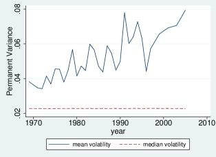
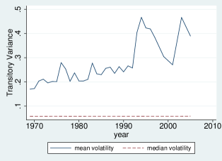
$99^{\mathrm{th}}$ Percentile	$99^{\mathrm{th}}$ Percentile
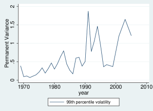
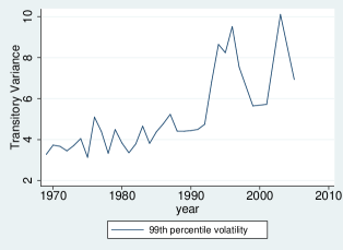
$90^{\mathrm{th}}$ and $95^{\mathrm{th}}$ Percentiles	$90^{\mathrm{th}}$ and 95th Percentiles
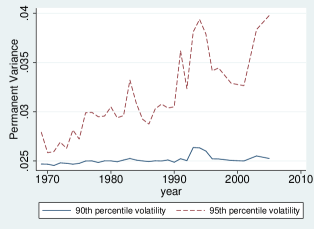
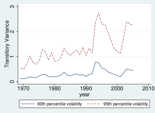
$\leq 75^{\mathrm{th}}$ Percentiles	$\leq 75^{\mathrm{th}}$ Percentiles

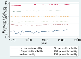
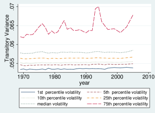
These figures show the evolution of various percentiles of the posterior mean of the permanent (left) and transitory (right) variance for various percentiles of the distribution of variance parameters.

4.3 Heterogeneity or fat tails?

So far, we have shown that the increases in income volatility can be attributed solely to increases in the right tail of the volatility distribution.  To obtain this result, our model assumes that the distribution of shocks is normal conditional on the volatility parameters.  When the unconditional distribution of shocks is fat-tailed (has high kurtosis), this is automatically attributed to heterogeneity in volatility parameters.  An alternative hypothesis is that there is little or no heterogeneity in volatility parameters, but that shocks are conditionally fat-tailed.

When looking at the cross-section of income changes, heterogeneity in volatility parameters (with conditionally normal shocks) and conditionally fat-tailed shocks (without no heterogeneity in volatility parameters) are observationally equivalent; they both imply a fat-tailed unconditional distribution of income changes.  By examining serial dependence, it is possible to reject the hypothesis that everyone has the same volatility parameter.  If shocks are conditionally fat-tailed but everyone has the same volatility parameters, then those with large past income changes should be no more likely than others to experience large subsequent income changes.  If individuals differ in their volatility parameters and those volatilities are persistent, then individuals with large past income changes will be more likely than others to have large subsequent income changes.

This possibility is investigated in Table 4 and shown graphically in Figure 1.  These compare the sample variance of income changes for individuals with and without large past income changes.  In each year, a cohort without large income changes is formed as the set of individuals whose measure of variance, either permanent variance or squared income change, was below median four years ago; a cohort with large income changes is formed as the set of individuals whose measure of variance was above the 95^th percentile four years ago.  This four-year period is chosen so that income shocks are far enough apart to be uncorrelated. (AbowdCard89)

Note that individuals with large past income changes tend to have larger subsequent income changes.  The tendency to have large income changes is persistent, which indicates that some individuals have ex-ante more volatile incomes than others.

The divergence over time in volatility between past low- and high-volatility cohorts is clear in both Figure 1 and Table 4.  The magnitude of income changes has been increasing more for those with large past income changes (who are more likely to be inherently high-volatility) than for those without such large past income changes (who are not).  This increase in volatility falls primarily on those who could be expected to have volatile incomes to begin with.  This shows that the increase in volatility among the volatile we find in the model cannot be attributed to increasingly fat-tailed shocks for everyone.

Table 7: Determinants of High Income Volatility (Probit)

Dependent	Permanent	Transitory
Variable	Variance	Variance
self-employed? 1 or 0	0.6001	0.7794
	(24.07)***	(32.22)***
	$[0.1085]$	$[0.1533]$
risk-tolerant? 1 or 0	0.1303	0.0950
	(5.91)***	(4.31)***
	$[0.0180]$	$[0.0131]$
age	0.0104	0.0082
	(7.82)***	(6.20)***
	$[0.0014]$	$[0.0011]$
years of education	-0.0041	-0.0123
	(-0.89)	(-2.67)***
	$[-0.0006]$	$[-0.0017]$
income$>$median? 1 or 0	-0.2277	-0.2922
	(-9.84)***	(-12.65)***
	$[-0.0308]$	$[-0.0398]$
have children? 1 or 0	-0.0498	-0.0686
	(-1.48)	(-2.04)**
	$[-0.0068]$	$[-0.0094]$
number of children	0.0120	0.0068
	(0.90)	(0.51)
	$[0.0016]$	$[0.0009]$
married? 1 or 0	-0.1009	-0.1815
	(-3.00)***	(-5.56)***
	$[-0.0143]$	$[-0.0270]$
$R^{2}$	0.0469	0.0751
observations	31,898	31,898

Results from a probit regression to predict an indicator variable for whether posterior mean variance (permanent or transitory volatility) estimate is is above the 90^th percentile for that year.  “Risk tolerant” is set to 1 if the PSID risk tolerance variable exceeds 0.3.   Above-median income indicates that four-year lagged income is above-median for that (lagged) year.   *, **, and *** indicate significance at the 10$\%$, 5$\%$, and 1$\%$ levels, respectively.  z-statistics are in parentheses.  Marginal effects are in square brackets.

4.4 Whose incomes are volatile?

In this paper, we have identified increasing volatility for men in the U.S. since 1968 as being driven solely by the right (volatile) tail of the volatility distribution.  Here, we examine the attributes of men with highly volatile incomes.

Table 7 presents the results from a probit regression to predict whether a person-year estimate of the (posterior mean) volatility parameter is above the 90^th percentile for that year.  Note from the first row that self-employed individuals are much more likely to have highly volatile incomes.  The second row shows that “risk tolerant” individuals are also much more likely to have highly volatile incomes.  Risk tolerance is identified from answers to hypothetical questions about lotteries, designed to elicit the individual’s coefficient of relative risk-aversion; risk-tolerant individuals are defined as those with an estimated coefficient of relative risk-aversion below 1/0.3.

High income individuals (those with incomes above median four years before the observation in question) are less likely to have volatile incomes.  Individuals with more years of education are also less likely to have volatile incomes.  Older individuals are more likely to have volatile incomes, a result driven by the large number of high-volatility individuals between ages 50 and 60.  Unsurprisingly, men who are married and/or who have children are less likely to have volatile incomes.

4.5 Whose incomes are increasingly volatile?

Section 4.4 identified attributes of individuals with volatile incomes.  In particular, the self-employed and those whose answers to survey questions suggest they are risk-tolerant are more likely to have volatile incomes.  Here, we examine the increase in volatility over time among these groups.

Table 8: Volatility Trends by Self-Employment, Income, and Risk Tolerance

Permanent Variance

	Self-Employment			Income			Risk Tolerance
	self-	not self-		$>$ med.	$\leq$ med.		risk	not risk
sample	employed	employed		income	income		tolerant	tolerant
change per year	0.0048	0.0011		0.0018	0.0009		0.0035	0.0012
$\%$ change ’68-’05	194$\%$	58$\%$		135$\%$	36$\%$		172$\%$	76$\%$
	(6.17)***	(4.58)***		(5.99)***	(2.75)***		(4.61)***	(4.50)***
N	6,068	41,766		10,336	23,876		23,958	18,029

Transitory Variance

	Self-Employment			Income			Risk Tolerance
	self-	not self-		$>$ med.	$\leq$ med.		risk	not risk
sample	employed	employed		income	income		tolerant	tolerant
change per year	0.0262	0.0061		0.0040	0.0116		0.0100	0.0076
$\%$ change ’68-’05	176$\%$	101$\%$		125$\%$	101$\%$		117$\%$	114$\%$
	(11.27)***	(13.80)***		(10.84)***	(13.22)***		(7.81)***	(9.45)***
N	6,068	41,766		23,876	23,958		10,336	18,029

Results from a weighted OLS regression to predict the posterior mean variance (volatility) estimate with a linear time trend.  The “change” row shows the coefficient on calendar time; the “percent change” row shows the expected percent change over the sample implied by this coefficient.  This is (100 percent) times (2005 minus 1968) times (the coefficient on calendar time) divided by (the average posterior mean in the sample).  The top panel presents results for the permanent variance; the bottom panel presents results for the transitory variance.  Each column presents results for a different sub-sample.  “Risk tolerant” means that the PSID risk tolerance variable exceeds 0.3.   Above-median income indicates that four-year lagged income is above-median for that (lagged) year.  t-statistics are in parentheses.

Table 9: Volatility Trends by Age and Education

Permanent Variance age education less than at least more than high less than sample 40 yrs old 40 yrs old high school school high school mean change/year 0.0006 0.0018 0.0024 0.0005 0.0004 $\%$ change ’68-’05 44$\%$ 76$\%$ 120$\%$ 28$\%$ 22$\%$ (3.66)*** (4.55)*** (6.08)*** (1.71)* (1.17) median change/year 0.0000 0.0000 0.0000 0.0000 0.0000 $\%$ change ’68-’05 0$\%$ 0$\%$ 1$\%$ 0$\%$ 0$\%$ (0.79) (4.29)*** (5.20)*** (-1.36) (0.20) 95^th $\%$tile chnge/year 0.0007 0.0010 0.0008 0.0007 0.0012 $\%$ change ’68-’05 53$\%$ 67$\%$ 63$\%$ 55$\%$ 72$\%$ (8.35)*** (6.47)*** (10.32)*** (6.50)*** (2.31)** N 23,928 23,906 23,455 15,516 8,863


Transitory Variance age education less than at least more than high less than sample 40 yrs old 40 yrs old high school school high school mean change/year 0.0057 0.0096 0.0093 0.0065 0.0066 $\%$ change ’68-’05 86$\%$ 123$\%$ 120$\%$ 102$\%$ 95$\%$ (9.36)*** (13.27)*** (12.14)*** (8.76)*** (6.91)*** median change/year 0.0000 0.0000 0.0000 0.0000 0.0000 $\%$ change ’68-’05 1$\%$ 2$\%$ 2$\%$ 2$\%$ 3$\%$ (6.87)*** (18.73)*** (11.18)*** (13.69)*** (7.60)*** 95^th $\%$tile chnge/year 0.0378 0.0649 0.0598 0.0483 0.0467 $\%$ change ’68-’05 124$\%$ 211$\%$ 183$\%$ 188$\%$ 135$\%$ (7.87)*** (17.10)*** (12.15)*** (11.04)*** (5.78)*** N 23,928 23,906 23,455 15,516 8,863

Results from a weighted OLS regression to predict the posterior mean variance (volatility) estimate with a linear time trend.  The “change” row shows the coefficient on calendar time; the “percent change” row shows the expected percent change over the sample implied by this coefficient.  This is (100 percent) times (2005 minus 1968) times (the coefficient on calendar time) divided by (the average posterior mean in the sample).  The top panel presents results for the permanent variance; the bottom panel presents results for the transitory variance.  Each column presents results for a different sub-sample.  t-statistics are in parentheses.

Table 8 predicts the posterior mean variance (volatility) estimates described earlier with a linear time trend.  The “change” row shows the coefficient on calendar time; the “percent change” row shows the expected percent change over the sample implied by this coefficient.  The top panel presents results for the permanent variance; the bottom panel presents results for the transitory variance.  Each column presents results for a different sub-sample.  By comparing the first two columns, note that that volatility has increased dramatically more for self-employed people than for others.  These individuals have much higher average levels of volatility, but their percentage change in volatility is still higher than for other individuals.  Self-employed individuals account for a substantial proportion of the overall increase in income volatility.  Similarly, the increase in permanent volatility (the variance of permanent shocks) is much greater for those who self-identify as risk tolerant (those whose estimated coefficient of relative risk aversion less than $1/0.3$) than those who do not.  Transitory volatility does not show major differences in trend for risk tolerant and not risk tolerant individuals.

Table 8 shows that the increase in volatility is apparent throughout the income distribution.  While increases in the average variance of transitory shocks are similar (in proportional terms) for those with above- and below-median income, the variance of permanent shocks has increased more for those with above-median income than for those with below-median income.  While below-median individuals are over-represented among those with the highest volatilities (Section 4.5), low income individuals are not driving the increase in volatility among those with the most volatile incomes.

Table 9 presents results by age and educational attainment.  Note that while magnitudes vary, the increase in volatility at the right tail is present for those below and above 40, and across the education distribution.

5 Conclusion

Increases in the size of income changes in the PSID can be attributed almost entirely to the “right tail” of the volatility distribution.  Taking volatility as a proxy for risk, those who would have had risky incomes in the past now face even more risk.  Everyone else has had no substantial change.

Without knowing more, the welfare implications of this finding are unclear.  Depending on what kind of people have volatile incomes, an increase in volatility at the volatile end of the distribution could be more or less bad than an increase in volatility for everyone.  Consider the possibility (which we refute in Section 4.4) that risk tolerance is independent of income volatility or expected income.  In this case, increasing volatility at the volatile end of the distribution decreases welfare more than increasing risk throughout the distribution.  When individuals have decreasing absolute risk aversion, high levels of income risk (proxied here by volatility) make people more vulnerable to additional risk. (Gollier2001)  If there is a compensating differential for risk so that volatile incomes are also higher on average, then this effect will be mitigated or reversed.

This paper shows that those with the most volatile incomes are also the most risk-tolerant.  In this case, the increase in risk has hit those best able to handle it. To the degree that income volatility is chosen (e.g., by choosing an occupation), we would expect those with the highest tolerance for risk or the best risk-sharing opportunities to take on the most volatile incomes.  If it is these individuals whose volatility has increased, it could blunt substantially any welfare costs associated with increased income volatility.   Since the increase in volatile has fallen disproportionately on the self-employed, it could also reflect an increase in profitable (but volatile) business opportunities.  In this case, there could even be welfare gains associated with increased income volatility.