A New FUSE Survey of Interstellar HD

Abstract

We have used archival FUSE data to complete a survey of interstellar HD in 41 lines of sight with a wide range of extinctions. This follow up to an earlier survey was made to further assess the utility of HD as a cosmological probe; to analyze the HD formation process; and to see what trends with other interstellar properties were present in the data. We employed the curve-of-growth method, supported by line profile fitting, to derive accurate column densities of HD. We find that the N(HD)/2N(H₂) ratio is substantially lower than the atomic D/H ratio and conclude that the molecular ratio has no bearing on cosmology, because local processes are responsible for the formation of HD. Based on correlations with E(B-V), H₂, CO, and iron depletion, we find that HD is formed in the densest portion of the clouds; the slope of the logN(HD)/log(H₂) correlation is greater than 1.0, caused by the destruction rate of HD declining more slowly than that of H₂; and, as a sidelight, that the depletions are density dependent.

1 Introduction

The H₂ isotopologue HD was first detected in Copernicus spectra by Spitzer et al. (1973, 1974) and Morton (1975), and has subsequently been observed in many sightlines by FUSE. The HD lines arising from the lowest-lying rotational levels ($J$=0 and $J$=1) are far weaker than their counterparts for H₂, but are in many cases still strong enough to be saturated, requiring a curve-of-growth analysis for column density determinations. To date HD analyses from FUSE spectra have been published only for a few stars Ferlet et al. (2000); Lacour et al. (2005) though many more detections reside in the FUSE archives. In addition, Lacour et al. have re-analyzed Copernicus spectra for several stars, resulting in a uniform survey of HD abundances in some 17 sightlines. The Copernicus stars generally have A_V values of 1.0 or less, while our FUSE targets cover a range of A_V from 0.1 to about 3 magnitudes.

The ratio of HD to H₂ — more specifically, N(HD)/2N(H₂) — in the Lacour et al. survey ranges from a few times 10^-7 to several times 10^-6. This is somewhat higher than the values found earlier from Copernicus data, but those values were based on two strong lines that were almost always saturated.

We follow the convention of Lacour et al. (2005), and assert that, in a region where all hydrogen (including deuterium) is in molecular form, the atomic D/H ratio is the same as the N(HD)/2N(H₂). The reasoning is that the molecular fraction (N(HD)/N(H_total) = N(HD)/[N(H I) + 2N(H₂)]) reduces to N(HD)/2N(H₂) when H I can be neglected. For every HD molecule, there is one D atom, so the atomic ratio D/H is equal to N(HD)/2N(H₂). Note that this assumes that not only H I, but also atomic D, can be neglected. This simplifying assumption is justified in cloud cores, but it may break down in regions where hydrogen (and deuterium) is only partially in molecular form, which may include some of the less-reddened lines of sight in our survey. But even there, as shown in the next few paragraphs, we can not use HD as an indicator of the D/H ratio anyway.

It would be useful if the N(HD)/2N(H₂) ratio were a reliable indicator of the atomic ratio D/H, because the latter is an important probe of the early expansion rate of the universe and therefore valuable in cosmology. An excellent summary of the observed atomic D/H ratio and its cosmological implications can be found in Linsky et al. (2006). But for three distinct reasons the comparison of HD to H₂ is difficult to apply to the cosmological problem.

First, H₂ begins to be self-shielding much before HD, as a function of depth in a cloud. For example, H₂ becomes self-shielding at about N(H₂) = 10¹⁹ cm^-2 (which corresponds to N(HD) = 10^12-13 cm^-2) and a similar column density would be required for HD – which is incredibly unlikely. For HD to become self-shielding, the column density of H₂ would have to be of order 10²⁵ cm^-2! Even infrared observations of the quadrupole transitions at 2.4 $\mu$m would never reach this column density. The fact that HD is not protected from radiative dissociation acts to lower the N(HD)/2N(H₂) with respect to the atomic D/H ratio in the denser portions of the lines of sight.

Second, if formation of HD occurs on grain surfaces (in parallel with H₂ formation), the lower mobility of D atoms on grains as compared to H atoms, greatly reduces the formation rate of HD as compared to H₂, acting to reduce N(HD)/2N(H₂) ratio relative to the D/H ratio. If grain formation of HD dominates, this would act to decrease the N(HD)/2N(H₂) ratio over the atomic ratio. For a more complex and complete analysis of HD formation on grain surfaces, see Cazaux et al. (2008).

But third, HD has a gas-phase formation channel, through the ”chemical fractionation” reaction H₂ + D${}^{+}\to$ HD + H⁺ Watson (1973); Le Petit et al. (2002), which tends to enhance the N(HD)/2N(H₂) ratio and depends on the cosmic-ray ionization rate Black & Dalgarno (1973). The comparison of the N(HD)/2N(H₂) ratio to the atomic D/H ratio can tell us which processes are most important.

In any case, the N(HD)/2N(H₂) ratio should not be expected to reflect the D/H ratio (Lacour et al. 2005). In general the N(HD)/2N(H₂) ratio is not useful for determining the cosmological D/H ratio, although it may be useful in constraining the rate of cosmic-ray ionization (which produces D⁺).

This paper, then, presents a new and more complete survey of HD than was available previously, to test formation theories and possible correlations with other interstellar quantities. We have organized the paper into sections as follows: Observation and Data Reduction, Data Analysis, Determination of HD Column Densities, Correlations, Summary and Conclusions.

2 Observation and Data Reduction

The FUSE mission covered a wavelength range (905-1188 Å) rich in ground state transitions, making it one of the most useful tools to study the interstellar medium. The 41 sightlines for this survey are archival FUSE spectra, chosen to span different cloud types and physical conditions. The sightline parameters used to select targets included color excess (0.11 $\leq$ $E(B-V)$ $\leq$ 0.83), the indicator of grain size R_v (2.25 $\leq$ $R_{v}$ $\leq$ 4.76), molecular fraction (0.02 $\leq$ f_H2 $\leq$ 0.76), and H₂ column density (19.07 $\leq$ log N(H₂) $\leq$ 21.11). Table 1 lists all of the relevant physical properties for the sightlines included in this study. Another selection criterion was a high signal-to-noise ratio around the 1105.83 Å HD line. This line is 100 times weaker than the rest of the HD absorption features measured, all of which have similar oscillator strengths (HD f-values and wavelength data from Abgrall & Roueff 2006). In many cases this weak line’s equivalent width is the only one falling on the linear portion of the curve of growth, thus providing unambiguous information about the column density as Lacour et al. found in their study.

Because HD is known to be correlated with H₂ abundances Lacour et al. (2005), our target list includes sightlines with H₂ column densities in the literature. H₂ column densities are taken from Shull et al. (in preparation, 2008) and Rachford et al. (2002; in preparation, 2008). For this study the FUSE data (Table 2) were pre-calibrated with version 3.1.4 or newer of the CALFUSE pipeline. For each observation we used a cross correlation analysis to align individual exposures with strong absorption features before co-adding them.

In most cases we co-added the detector segments to increase the signal to noise ratio before measuring the HD equivalent widths. When combining the detector segments one significant systematic flaw was found in the data. The raw data from the LiF2A detector segment revealed the same systematic detector defect due to a Type I dead zone (as described in section 9.1.6 of The FUSE Instrument and Data Handbook) in all sightlines in the vicinity of the weak 1105.83 Å HD line; thus we excluded that segment and only used LiF1B.

3 Data Analysis

To determine the column density of HD we measured equivalent widths for all possible HD lines (see Table 4) and performed a curve of growth (COG) analysis. All of the HD lines measured are transitions from the ground rotational state ($J$=0). While there are over 25 HD absorption lines in the FUSE range, only seven are isolated enough from other features to determine accurate equivalent widths. To measure the equivalent width we first defined a continuum on both sides of the feature and normalized it with low order (1 to 3) Legendre polynomials. When there was no other absorption feature in the immediate vicinity we integrated over the HD line while summing the flux errors provided by FUSE in quadrature. If there was another absorption feature blended with the HD line, we fit the HD and interfering line with Gaussians (see next section for details). The errors in the width and depth of the Gaussian were propagated into the equivalent width error. The statistical error on the equivalent width was summed in quadrature with the continuum placement error. The continuum error was up to an order of magnitude smaller than the statistical error in all cases.

Of the seven lines, six have similar oscillator strengths (see Table 5); the seventh and weakest line is located at 1105.86 Å and is very important for constraining the COG fit. The weak HD line is difficult to measure in most cases and in other cases it is impossible to measure at all. Without a line to measure we used the signal-to-noise ratio to set a two sigma upper limit on the equivalent width using the equation:

$$\sigma=\frac{\Delta\lambda M^{1/2}}{(S/N)}$$ (1)

where $\Delta\lambda$ is the pixel scale, $S/N$ is the signal-to-noise ratio, $M$ is the width of the feature (here FUSE resolution elements ($\sim$9 pixels) are used since the width of the line will be smeared out by the resolution), and $\sigma$ gives the one sigma error of the equivalent width Jenkins et al. (1973).

3.1 Modeling the C I* Line

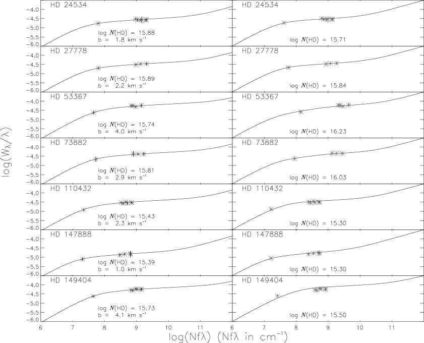
Figure 1: Single Component (left) and Multiple Component (right) Curves of Growth for HD 24534 through HD 149404.

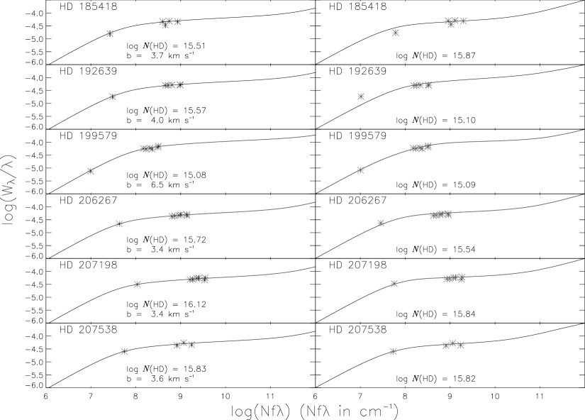
Figure 2: Single Component (left) and Multiple Component (right) Curves of Growth for HD 185418 through HD 207538.

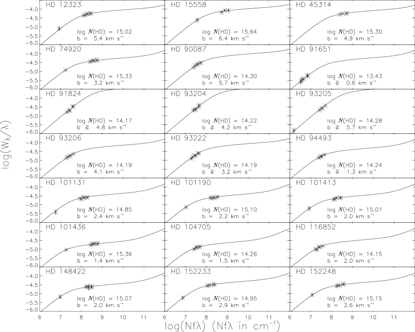
Figure 4: Single Component Curves of Growth with column densities and $b$-values for HD 12323 through HD 152248.

The first obstacle in measuring the weak HD line is a very crowded patch of continuum. In a study of the sightline to $\zeta$ Oph, Morton (1978) found an unidentified absorption feature at 1105.92 Å. In the current study we have been unable to confirm or deny the existence of a weak feature near this wavelength; thus, if such a feature does exist it could be a source of systematic error. Morton also rejected a feature at 1105.82 as being the weak line of HD due to its large equivalent width. The conclusion of Lacour et al. (2005) and the present study is that the feature at 1105.83 is indeed HD and its strength is consistent with all of the other measured HD features (see Figures 1, 2, 4 & 5 containing HD COG’s). Shortward of the HD line, by 0.13 Å, is an absorption feature from the first excited state of carbon as discussed by Lacour et al. In sightlines where the C I* and HD lines were blended we modeled the C I* and divided it from the spectrum before measuring the HD line.

Removing this blended C I* line turned out to be more challenging than originally thought. The f-value of the 1105.73 C I* line, previously measured as 0.0113 by Morton (1978), did not fit the curve of growth set by the other C I* lines. This is probably due to uncertainty in the adopted f-value of this weak line. The previous value was based on a single measurement of the line in the spectrum of $\zeta$ Oph. So to accurately model the C I* line we used existing archival data to make an empirical estimate of the f-value, based on more sightlines.

To accomplish this task we found Copernicus, FUSE, and/or STIS data in sightlines where the 1105 Å C I* line was well defined, not heavily blended with other lines in the region (HD 12323, $o$ Per, HD 207538, HD 210839) and measured the equivalent widths of all well defined C I* lines, excluding the 1105 Å line. For each sightline we then fit these equivalent widths to a single component curve of growth varying both $b$-value and column density (see Figure A New FUSE Survey of Interstellar HD for an example). Once a best fit curve of growth was found, the f-value of the 1105 Å line was calculated using its measured equivalent width. Uncertainty in the f-value was assigned based on errors in the measured equivalent width of the 1105 Å line. Calculated f-values and uncertainties for each sightline can be found in Table 6. The results from all sightlines were combined using a weighted average and the final f-value was found to be 0.0062${}^{+0.0015}_{-0.0010}$.

The C I* lines used in modeling are in Table 5. We used STIS data when available, along with FUSE data to measure the C I* absorption features. Using the best fit column density and $b$-value of C I*, we generated a Voigt profile of the 1105.73 Å C I* line. This profile was then convolved with the Gaussian instrumental profile (assuming a resolution of 20 km s^-1) and divided out of the spectrum, allowing us to measure the HD 1105.83 Å line.

We began the current study using C I* line f-values from Morton’s compilation (1991). However, in light of newer theoretical f-values from Zatsarinny & Froese Fischer (2002) and Froese Fischer (2006), it was important to determine whether differences due to revised f-values would substantially affect our HD column densities. Repeating the calculation of the C I* 1105.73 Å line f-value yielded only a very small change (about three percent) from the previously calculated f-value. All C I* column densities were also recalculated using the newer f-values. Total column densities did not vary greatly from those using the Morton (1991) f-values. In all but three cases differences in C I* column density using the two sets of f-values differed by 0.1 dex or less. The three most discrepant cases were HD 73882, HD 101436 and HD 149404. For these three cases the equivalent width of the weak HD line was remeasured and found to be well within the 1$\sigma$ errors of the previous measurements. Similarly, in all three cases rerunning the COG fit yielded only small changes in the HD column density that were within the 1$\sigma$ error bars of the previous measurements (in all cases the difference was less than 0.1 dex). Thus, we did not think it necessary to repeat all of the C I* modeling, and remeasure the weak HD line, as other errors far exceed any error introduced by minor changes in some of the C I* f-values, and changes in C I* column densities were not substantial in the vast majority of cases. All reported C I* column densities are those using the newer f-values from Zatsarinny & Froese Fischer (2002) and Froese Fischer (2006).

4 Determination of HD Column Densities

Once the influence of C I* had been removed, we were able to do a curve-of-growth analysis to determine the column density, but we used profile fitting in a few cases as a check. We did two different COG analyses; multiple component COG’s for a sub-set of 13, and single component COG’s for all 41 sightlines. Both are described below in subsection 4.1 ’Curve of Growth Analysis’. The profile fitting is described in subsection 4.2.

4.1 Curve of Growth Analysis

In many cases multiple cloud components exist along a single line of sight increasing the difficulty in accurately measuring the column density. Having knowledge of such structure is most important when the equivalent widths fall on the flat portion of the curve. We can create a multiple component COG, but first we need to find a suitable tracer of HD.

HD has been found to be correlated to H₂ Lacour et al. (2005). Similarly CH is traced by H₂ because of the chemistry: the creation of CH in the diffuse ISM is directed through a series of gas phase reactions with H₂ (Danks, Federman & Lambert 1984; van Dishoeck & Black 1989; Magnani et al. 1998). Since CH and HD are both correlated to H₂ abundances, there is an inferred correlation between CH and HD, which has been verified by Lacour et al.

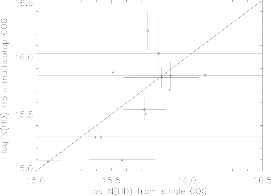
Figure 3: Column Density solutions from a multiple component curve of growth compared to a single component curve of growth.

For thirteen sightlines we had high resolution CH data (Welty, private communication) which we used to define a velocity structure for HD. From the measured CH line-of-sight velocity structure, we generated multiple component COG’s. The HD equivalent widths were fit to the curve varying only the total column density. For comparison the data were also fit to a single component COG that found a best fit of both $b$-value and column density by minimizing the ${\chi}^{2}$. Figures 1 and 2 show the side by side comparison of the COG analyses, and Figure 3 compares the column densities and errors from the two methods.

The COG’s from the two methods fit the data in all but three cases. The side by side comparison show a clear mis-fit of the multiple component COG for HD 149404, HD 185418, HD 192639, even though the column densities are within one-sigma errors for the first two targets. The discrepancy arose because a multiple component COG assumes the best fit velocity structure of CH is the actual structure of the HD and does not allow for errors. Varying the $b$-values on the multiple component COG within their one sigma errors gave solutions that were consistent with the data and the single component COG.

With the reasonable assurance that our single component COG model is good we accounted for any other systematic errors that we could not quantify by setting the reduced $\chi^{2}$ of the best-fit curve equal to one. In 22 sightlines the reduced $\chi^{2}$ was already less than one, thus the errors were unchanged; for the remaining 19 cases the assumed good fit scaled up the errors in equivalent width and column density.

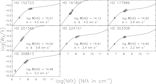
Figure 5: Single Component Curves of Growth with column densities and $b$- values for HD 152723 through HD 308813.

The consistency between the results of the single and multiple component COG demonstrates that a single component model is a good approximation when we do not have component information. Thus, we are justified in combining the HD results for the 13 targets with component information and the 28 targets without; see Figures 4 and 5 for single component COG’s and Table 7 for column densities.

Solving for column density in the COG analysis was more complicated when we only had an upper limit on the 1105 Å line. We used the limit on the weak line to constrain the column density by throwing out solutions beyond the upper limit. The limit was not used in calculating the $\chi^{2}$ of the fit.

Lower limits on the $b$-value were determined when all the points fell on the linear portion of the COG. The $b$-value controls where the curve will transition from the linear to the saturated portion. Since the transition cannot occur lower than the data points a two sigma lower limit is set (HD 91824, HD 93204, HD 93205, HD 94493, HD 161807, and HD 201345.)

4.2 Profile Fitting

Profile fitting of the HD lines was done for five lines of sight to verify the COG column density measurements. All the available HD lines were fit simultaneously so that a single best fit column density and $b$-value would be measured. First the continuum surrounding each HD feature was normalized by fitting a low order Legendre polynomial to the continuum on both sides. Shifts in the central velocity of the HD features were noticed from one line to another, (with each detector segment showing different velocity shifts, usually on the order of $\sim$10 km s^-1) so the lines were each fit with a single Gaussian and the central wavelength corrected so that each feature would be at its rest wavelength. Profiles were modeled assuming a single Voigt profile with column density $N$, line width $b$ and central velocity $v$. These profiles were then convolved with a Gaussian instrumental profile. We used the non-linear least-squares curve fitting algorithm MPFIT by C. Markwardt to find the best fit parameter values. MPFIT is a set of routines that uses the Levenberg-Marquardt technique to minimize the square of deviations between data and a user-defined model. These routines are based upon the MINPACK-1 Fortran package by More’ and collaborators.

Attempts were also made to fit multiple components when previous measurements of CH existed. However, even when the velocity structure was fixed by the CH structure, individual component column densities did not converge to reasonable answers. Usually one component of the fit dominated while the other component(s) were an order of magnitude or two lower in column density (differing greatly from the relative strengths of the CH components). Because of this, we report only the single component fits in Table 8.

For all five sightlines we find that the column densities and $b$-values for both the curve of growth and profile-fitting method are within standard errors of one another (including HD 192639, our previously discrepant case). We also find that the best fit profiles match the absorption profiles in the data well (see Figure 6). Thus, we are confident that our column densities measured through curve of growth fitting are reliable.

4.3 Comparisons with previous results

We are able to compare our column densities with the previous HD survey of Lacour et al. (2005). This survey had 7 stars observed with FUSE and 10 more lines of sight observed years before, with Copernicus. The comparison of our results are in Table 3.

We re-analyzed the 7 FUSE targets that Lacour measured to check whether our method was consistent with their results. Our method differs in a few small ways. We re-derived the C I* f-value (as described above), so our de-blending of the weak HD line is different. Also we weighted each line equally in the COG fit, while the Lacour group doubly-weighted the optically thin HD line. Even with these difference our column densities are consistent within the uncertainties.

We also did single-component curves of growth for every sightline, which the Lacour group did not, and we found consistent column densities with the multicomponent results. This allowed us to expand our survey with confidence, in the end obtaining accurate column densities for 41 stars.

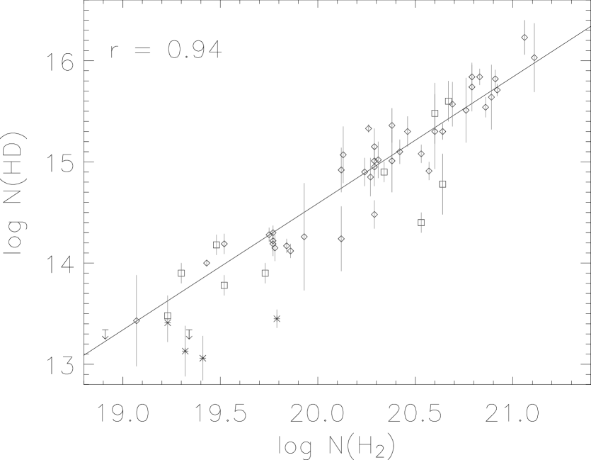
Figure 7: Correlation plots of log N(HD) versus log N(H₂). The line is a weighted least-squares fit. Square plot symbols represent Copernicus data analyzed by Lacour et al. 2005, diamonds represent this study, asterisk and upper limit represent Copernicus data reported by Spitzer et al. 1974.

Previous HD measurements made by Spitzer et al. (1974) are included in Figure 7 and the correlation analysis. The plot includes the upper limits for $\delta$ Per and $\lambda$ Ori and the measurements for $\pi$ Sco, $\delta$ Sco, $\sigma$ Sco, and $\gamma$ Ara.

5 Correlations

One way to derive information about the formation mechanism of HD, and to test theoretical chemical models, is to see how various interstellar quantities correlate with HD column densities. Before we do that, a few words of caution are in order. Of necessity, we can measure only integrated line-of-sight quantities, not localized to the same portion of the lines of sight. For example, any correlations of molecular quantities versus dust indicators or H I are probably not informative, because both dust and H I are everywhere, inhabiting every region from diffuse to dark clouds. We assume, with good reason, that the observable HD and H₂ (along with CH) are confined to diffuse molecular and translucent clouds (as defined by Snow & McCall 2006), so we should not expect to find good correlations with either dust or H I. If we do find good or decent correlations, that would indicate that diffuse molecular and translucent clouds dominated the lines of sight in our survey. On the other hand, those quantities that do correlate well with each other would show that they arise in the same portion of the line of sight. All correlations can be found in Table 9, including some not illustrated.

The first correlation of interest is the one between HD and H₂, which is shown in Figure 7. There we see a very good correlation, suggesting that the formation of HD depends on the local abundance of H₂, or that both are formed by the same or similar processes. Because H₂ shoots up in column density due to the self-shielding about when N(H₂) reaches 10¹⁹ cm^-2, we checked for a change in slope around that point. We see more scatter below log N(H₂) = 19.5 and no significant change in slope (below 19.5, the slope is 1.55, based on a fairly narrow range; above, it is 1.33). Considering all of our data points together gives an overall slope of 1.25 and a correlation coefficient is 0.94.

The significant departure from a slope of 1.00 in this correlation can be interpreted in two different ways: either HD is being formed at a faster rate than the formation rate of H₂ in the portion of the clouds where both are forming; or HD is destroyed at a lesser rate than the destruction rate of H₂ in those regions. This latter explanation may be preferred, because of optical depth effects and how they affect the photodestruction rates. For most of the observed range in A_V, the H₂ $J$ = 0 and 1 lines are damped, while the corresponding lines of HD lines are becoming saturated - but not damped. In this range in A_V (between A_V about 0.1 and 0.8), the rate of HD destruction is rapidly declining, while the photodestruction rate of H₂ is only slightly declining Le Petit et al. (2002). This situation mimics the appearance of relative rate of formation favoring HD, and that explains the slope of the N(HD)/N(H₂).

The alternative explanation of the slope in Figure 7, that HD is being formed faster than H₂, could only be viable if some additional formation process were at work, in addition to the standard gas-phase reaction network. And that would imply HD formation on grain surfaces competes with the gas-phase mechanism. But the detailed analysis of HD formation on grains by Cazaux et al. (2008) explores conditions in which grain formation of HD could be important, and our observed lines of sight do not meet the criteria outlined by Cazaux et al. So our explanation, that HD has started to be destroyed at a lesser rate, is more likely.

This finding of a greater slope than 1.00 seems to be inconsistent with the gas-phase models of Le Petit et al. (2002), who predict that the ratio of HD over H₂ should decline over our entire range in molecular fraction. Their Figure 4 shows the ratio N(HD)/2N(H₂) as a function of the molecular fraction of hydrogen, and this figure shows a steady decline with increasing molecular fraction. Only above a molecular fraction of 0.9 does the ratio start to increase. The study by Le Petit et al. only considers a single cloud, whereas real sightlines cover many clouds in most cases. But it is difficult to see how this helps reconcile the model with the observations, because the situation only gets worse when multiple clouds, which collectively form the total column density, are considered. The model would be correct only if all the molecular regions along the lines of sight, each having a molecular fraction $\geq$ 0.9, contained all the HD and H₂, with no spillover to less dense regions.

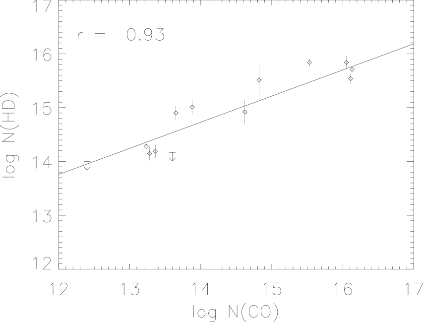
Figure 8: Correlation of log N(CO) with log N(HD). CO data from Burgh et al. 2007

Figure 8 shows the correlation between the column densities of HD and CO (the CO data were taken from Burgh et al. 2007). Here we see a very good correlation (coefficient 0.93), which we take as an indication that related processes account for both HD and CO. Since CO is formed by gas-phase reactions (e.g Kaczmarczyk 2000a; 2000b; and references cited therein), we again conclude that HD is also likely formed by gas-phase reactions. The ion-neutral reaction H₂ + D${}^{+}\to$ HD + H⁺ Le Petit et al. (2002), with the ion D⁺ being created by cosmic-ray impacts, is commonly thought to be the primary gas-phase formation channel for HD.

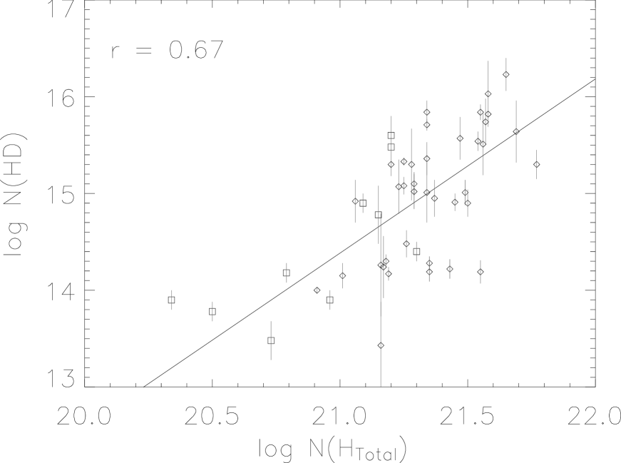
Figure 9: Correlation plots of log N(HD) versus log N(total Hydrogen). Square plot symbols represent Copernicus data analyzed by Lacour et al. 2005, diamonds represent this study.

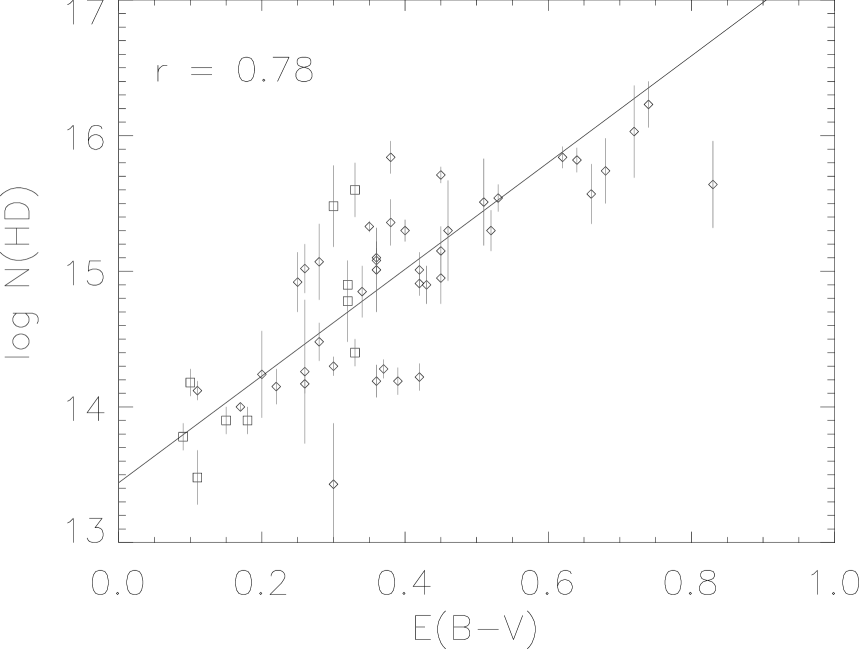
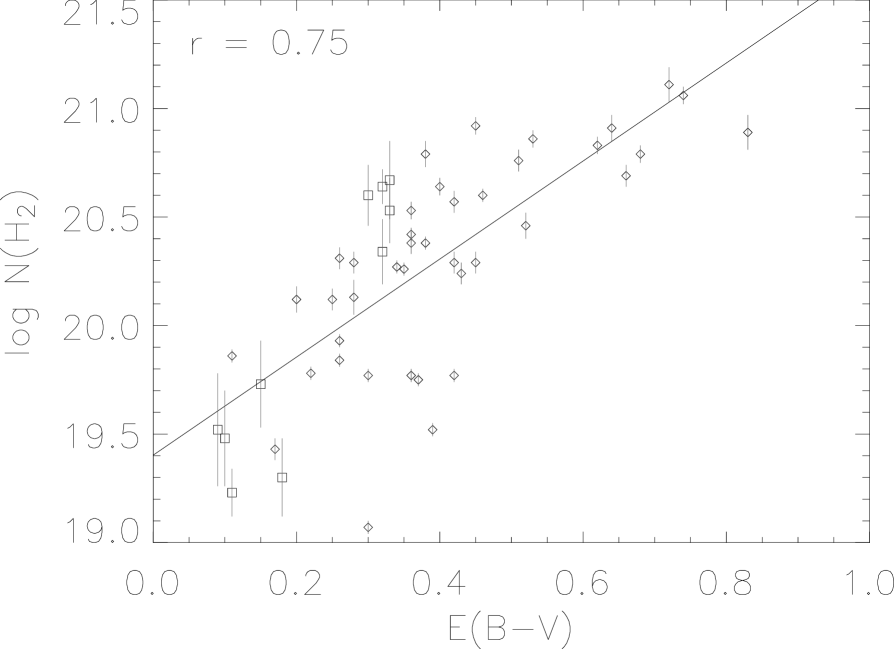
Figure 10: log N(HD) and log N(H₂) versus reddening, E(B-V). Symbols same as Figure 9.

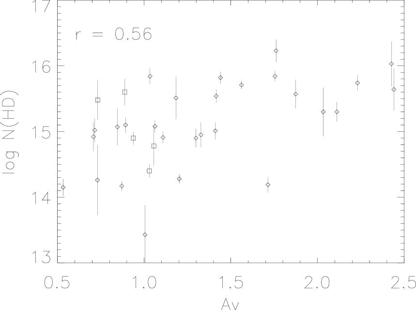
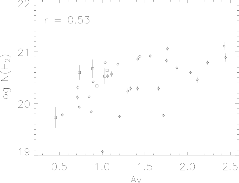
Figure 11: log N(HD) and log N(H₂), versus extinction (A_V). Symbols same as Figure 9.

To test our assertion that HD and H₂ do not inhabit the whole line of sight in most cases, we show the correlations of both with quantities that are expected to arise over the entire sightline. In Figure 9 we show the correlations of HD with the dust parameters total H (i.e., N(H I) + 2N(H₂)); Figure 10 shows the correlations of H₂ and HD with E(B-V); and Figure 11 shows the correlations of H₂ and HD with A_V. These correlations do not differ significantly from each other, except there is a hint that both HD and H₂ go with E(B-V) slightly better than they correlate with either total H, or A_V. Neither HD or H₂ correlate significantly with R_V.

The correlations of HD and H₂ with E(B-V) are better than those with H I, telling us something surprising and perhaps useful: that the grains responsible for differential extinction tend to be in the densest parts of the observed lines of sight, where HD and H₂ are present. The grains responsible for E(B-V) are thought to be comparable in size to the wavelengths being scattered, so we conclude that other grains in the lines of sight may have a different size distribution.

We tested correlations of both H₂ and HD against the molecular fraction, given by f = N(H₂)/N(H_Total), and found a fairly good correlation (see Table 9). Neither should be a surprise, because they just show that H₂ and HD exist primarily in the densest portions of the lines of sight, as expected.

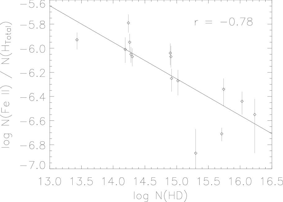
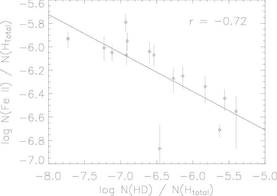
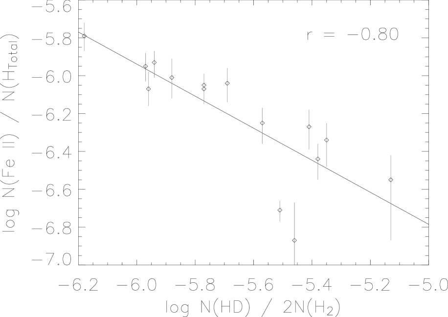
Figure 12: Correlations with iron depletions, a density indicator. Iron data in Table 1 originally reported by Jensen & Snow 2007.

Finally, we have looked at correlations between iron depletion, as shown by the ratio of iron to total hydrogen, and we see several interesting things. These correlations are shown in Figure 12. We could have considered correlations with depletions of other elements, but we have more complete data on iron for our lines of sight, and we expect other refractory elements to follow more or less the same trends as iron. The iron column densities come from Jensen & Snow (2007), and are listed in Table 1.

The three correlations we considered are consistent with the idea that the depletions are density dependent. Remembering that an increasingly negative value of the Fe/H ratio means more depletion of iron, we see that the depletion is growing with indicators of density such as the HD column density, the fractional ratio of HD (i.e., N(HD)/N(H_Total); and the ratio of HD to H₂ (see Figure 12). The indicators we see here, showing that depletion increases with density, is consistent with the finding of Burgh et al. (2007), who found that the depletions correlate with CO, another density indicator.

6 Summary and Conclusions

We have derived column densities of interstellar HD for 41 lines of sight, covering a wide range of total extinctions, total hydrogen column density, and differential extinction E(B-V). We went to considerable effort to reduce error in the derived column densities, which were ultimately found using the curve-of-growth method, after measuring the equivalent widths. One challenge we faced, and successfully resolved, was that the weakest line of HD, detectable only toward highly-reddened stars, was contaminated by a weak C I* line. We had to model and remove the C I* line in those cases. Where possible, we checked our results against other published column densities, with generally good agreement.

We found values of the logarithmic ratio of N(HD)/2N(H₂) ranging from -6.18 to -5.13 – generally much lower than the galactic atomic D/H ratio and even lower with respect to the extragalactic (or the primeval) ratios Linsky et al. (2006). This says two things: (1) the enhanced photodissociation of HD over H₂ dominates and lowers the N(HD)/2N(H₂) ratio; and (2) our initial assumption that we can not use N(HD)/2N(H₂) ratio as a cosmological test is confirmed, and only the atomic ratio gives a true value of the primordial production of deuterium (if that; see Linsky et al. 2006).

In order to see whether our results are consistent with extant chemical models, we examined correlations of HD with other interstellar parameters, finding the following: (1) HD is declining more slowly than the destruction rate of H₂; (2) N(HD) correlates well with N(CO); and (3) the depletion of iron (and probably other refractory elements) is enhanced in the densest portions of the lines of sight. The model of Le Petit et al. (2005) of the formation of HD is inconsisten with the observations, unless individual dense clouds along the lines of sight contain all the HD and H₂.

Table 1: Sightline Properties

Star	E(B-V)	$R_{V}$	Ref.	Molec.	log N(H2)	log N(CH)	log N(HTot)	Ref.	log N(Fe II)	log N(C I*)
(HD)				Fract.	(cm-2)	(cm-2)	(cm-2)		(cm-2)	(cm-2)
12323	0.26	2.75	1	0.21	20.31	…	21.29	4	15.02	…
15558	0.83	2.94	2	0.32	20.89	…	21.69	4	…	…
24534	0.45	3.47	3	0.76	20.92	13.57	21.34	5	14.63	14.98 $\pm$ 0.02
27778	0.38	2.72	3	0.56	20.79	13.48	21.34	5	…	15.15 $\pm$ 0.32
45314	0.46	4.42	1	0.42	20.60	…	21.28	4	…	…
53367	0.74	2.38	3	0.52	21.06	…	21.65	3	15.08	15.16 $\pm$ 1.83
73882	0.72	3.37	3	0.67	21.11	13.57	21.58	5	15.15	16.35 $\pm$ 0.64
74920	0.35	…	…	0.21	20.26	…	21.25	4	…	…
90087	0.30	…	…	0.08	19.77	…	21.18	4	15.15	…
91651	0.30	3.35	1	0.02	19.07	…	21.16	4	15.23	…
91824	0.26	3.35	1	0.09	19.84	…	21.19	4	…	…
93204	0.42	…	…	0.04	19.77	…	21.43	4	…	…
93205	0.37	3.25	1	0.05	19.75	…	21.35	4	15.35	14.13 $\pm$ 0.05
93206	0.39	…	…	0.03	19.52	…	21.35	4	…	14.13 $\pm$ 0.17
93222	0.36	4.76	1	0.03	19.77	…	21.55	4	…	13.77 $\pm$ 0.04
94493	0.20	…	…	0.18	20.12	…	21.17	4	15.38	…
101131	0.34	…	…	…	20.27	…	…	4	…	…
101190	0.36	2.48	1	0.27	20.42	…	21.29	4	…	14.54 $\pm$ 0.11
101413	0.36	…	…	0.22	20.38	…	21.34	4	…	…
101436	0.38	…	…	0.22	20.38	…	21.34	4	…	14.49 $\pm$ 0.22
104705	0.26	2.81	1	0.12	19.93	…	21.16	4	15.22	…
110432	0.40	…	…	0.55	20.64	13.19	21.20	5	…	14.55 $\pm$ 0.26
116852	0.22	2.42	1	0.12	19.78	…	21.01	4	…	…
147888	0.52	4.06	3	0.10	20.46	…	21.71	3	14.89	15.02 $\pm$ 0.10
148422	0.28	3.02	1	0.16	20.13	…	21.23	4	…	…
149404	0.68	3.28	3	0.33	20.79	…	21.57	3	15.23	14.86 $\pm$ 0.09
152233	0.45	2.95	1	0.17	20.29	…	21.37	4	…	…
152248	0.45	3.68	1	…	20.29	…	…	4	…	…
152723	0.42	3.36	1	0.13	20.29	…	21.49	4	…	…
161807	0.11	…	…	…	19.86	…	…	4	…	…
177989	0.25	2.83	1	0.23	20.12	…	21.06	4	14.81	14.52 $\pm$ 0.03
185418	0.51	2.32	3	0.47	20.76	13.12	21.56	5	…	14.35 $\pm$ 0.08
192639	0.66	2.84	3	0.32	20.69	13.45	21.47	5	…	14.54 $\pm$ 0.08
199579	0.36	2.95	3	0.38	20.53	13.36	21.25	5	…	14.78 $\pm$ 0.12
201345	0.17	…	…	0.03	19.43	…	20.91	6	…	…
206267	0.53	2.67	3	0.42	20.86	13.41	21.54	5	…	14.91 $\pm$ 2.09
207198	0.62	2.42	3	0.38	20.83	13.56	21.55	5	…	15.18 $\pm$ 0.16
207538	0.64	2.25	3	0.43	20.91	13.63	21.58	5	…	15.23 $\pm$ 0.15
224151	0.42	2.64	2	0.26	20.57	…	21.45	4	15.38	14.34 $\pm$ 0.06
303308	0.43	3.02	1	0.11	20.24	…	21.50	4	15.46	14.38 $\pm$ 2.61
308813	0.28	…	…	0.22	20.29	…	21.26	4	…	…

Table 2: Observation data

Star	Stellar	V	Dist	Ref.	FUSE Data ID	STIS Data ID
(HD)	Type	(mag)	(pc)
12323	O9V	8.92	3900	1	P1020202000
15558	O5IIIf	7.95	2187	2	P1170101000
24534	O9.5pe	6.10	398	2	P1930201000	o66p01020
27778	B3V	6.33	220	3	P1160301000	o59s01010
45314	O9pe	6.60	799	2	P1021301000
53367	BoIV:e	6.94	247	3	P1161101000
73882	O9III	7.24	925	1	P1161302000
74920	O8	7.54	1497	2	P1022601000
90087	O9.5III	7.80	2716	2	P1022901000
91651	O9Vn	8.87	3500	1	P1023102000
91824	O7V	8.15	4000	3	A1180802000
93204	O5Vf	8.48	2630	2	P1023501000
93205	O3V	7.76	2600	1	P1023601000	o4qx01030
93206	O9.7Ibn	6.24	2512	2	P1023401000
93222	O7IIIf	8.11	2900	1	P1023701000	o4qx02030
94493	B0.5Iab	7.27	3327	2	P1024101000
101131	O6Vf	7.16	709	3	P1024901000
101190	O6Vf	7.27	2399	2	P1025001000
101413	O8V	8.33	2399	2	P1025301000
101436	O6.5V	7.58	2399	2	P1025401000	o6lz51010
104705	B0Ib	7.83	3898	2	P1025701000
110432	B1IIIe	5.24	301	3	P1161401000
116852	O9III	8.49	4760	2	P1013801000
147888	B3	6.78	136	3	P1161501000	o59s05010
148422	B1Ia	8.64	8836	2	P1015001001
					P1015002001
					P1015003001
149404	O9Iae	5.47	1380	2	P1161702000
152233	O6III	6.59	1905	2	P1026702000
152248	O7Ibnfp	6.11	1758	4	P1026801000
152723	O6.5IIIf	7.31	1905	2	P1027102000
161807	B0IIIn	7.01	383	3	P1222302000
177989	B0III	9.34	4909	2	P1017101000
185418	B0.5V	7.45	950	5	P1162301000	o5c01q010
192639	O7Ib(f)	7.11	1100	1	P1162401000	o5c08t010
199579	O6Ve	5.96	794	2	P1162501000
201345	O9V	7.75	1907	2	P1223001000
206267	O6.5V	5.62	850	1	P1162701000
207198	O9.5Ib-II	5.96	832	2	P1162801000	o59s06010
207538	O9V	7.31	832	2	P1162902000	o63y01010
224151	B0.5II	6.05	1355	2	P1224103000	o54308010
303308	O3Vf	8.21	2630	2	P1221602000	o4qx04010
308813	O9.5V	9.32	2398	2	P1221903000

Table 3: Previously Reported HD Column Densities Comparison

	Previous Values	Our Values
Star	log N(HD)	log N(HD)
(HD)	(cm-2)	(cm-2)
27778	15.51 ${}^{+0.30}_{-0.33}$	15.84 $\pm$ 0.12
73882	15.76 ${}^{+0.21}_{-0.38}$	16.03 $\pm$ 0.34
110432	15.28 ${}^{+0.14}_{-0.17}$	15.30 $\pm$ 0.08
185418	15.63 ${}^{+0.16}_{-0.13}$	15.51 $\pm$ 0.32
192639	15.18 ${}^{+0.20}_{-0.27}$	15.57 $\pm$ 0.22
206267	15.32 ${}^{+0.23}_{-0.28}$	15.54 $\pm$ 0.10
207538	15.70 ${}^{+0.31}_{-0.28}$	15.82 $\pm$ 0.09

Table 4: Equivalent Widths of HD lines

Star	W959.82	W975.58	W1011.46	W1021.46	W1054.29	W1066.27	W1105.86
(HD)	(mÅ)	(mÅ)	(mÅ)	(mÅ)	(mÅ)	(mÅ)	(mÅ)
12323	43.9 $\pm$ 3.0	53.0 $\pm$ 3.8	60.4 $\pm$ 3.3	55.1 $\pm$ 2.5	55.0 $\pm$ 2.3	46.4 $\pm$ 3.0	8.7 $\pm$ 2.5
15558	…	…	…	86.0 $\pm$ 19.0	90.1 $\pm$ 12.5	70.3 $\pm$ 10.2	26.9 $\pm$ 7.6
24534	25.8 $\pm$ 5.2	26.5 $\pm$ 10.7	26.2 $\pm$ 4.2	28.4 $\pm$ 2.8	27.3 $\pm$ 1.8	32.3 $\pm$ 2.3	18.8 $\pm$ 1.4
27778	…	…	34.7 $\pm$ 5.6	…	35.4 $\pm$ 2.7	32.9 $\pm$ 4.4	22.0 $\pm$ 2.2
45314	…	…	57.0 $\pm$ 1.7	59.9 $\pm$ 1.4	59.2 $\pm$ 1.2	53.4 $\pm$ 1.1	$<$ 25.7
53367	53.8 $\pm$ 10.5	…	…	59.8 $\pm$ 15.8	51.9 $\pm$ 5.7	61.2 $\pm$ 8.6	26.3 $\pm$ 4.9
73882	…	…	…	43.0 $\pm$ 10.1	44.2 $\pm$ 6.3	45.6 $\pm$ 16.0	24.0 $\pm$ 8.0
74920	37.0 $\pm$ 3.3	38.9 $\pm$ 3.8	43.7 $\pm$ 1.9	42.2 $\pm$ 1.5	42.4 $\pm$ 1.7	36.0 $\pm$ 1.6	13.0 $\pm$ 0.8
90087	20.6 $\pm$ 2.0	26.1 $\pm$ 3.6	30.3 $\pm$ 1.4	30.7 $\pm$ 1.5	23.7 $\pm$ 1.2	17.5 $\pm$ 1.1	$<$ 4.9
91651	3.2 $\pm$ 1.4	…	5.3 $\pm$ 0.9	6.2 $\pm$ 1.3	3.9 $\pm$ 0.8	2.9 $\pm$ 1.0	…
91824	15.4 $\pm$ 2.3	19.1 $\pm$ 2.6	34.1 $\pm$ 6.9	33.7 $\pm$ 2.3	21.7 $\pm$ 1.7	…	$<$ 3.8
93204	19.8 $\pm$ 5.0	23.9 $\pm$ 4.1	41.5 $\pm$ 4.4	32.4 $\pm$ 6.8	23.1 $\pm$ 2.2	…	$<$ 4.5
93205	19.8 $\pm$ 1.3	26.6 $\pm$ 1.5	37.6 $\pm$ 1.4	…	27.4 $\pm$ 1.0	…	1.6 $\pm$ 0.6
93206	14.8 $\pm$ 1.5	18.3 $\pm$ 2.2	23.2 $\pm$ 1.5	…	17.7 $\pm$ 0.6	14.1 $\pm$ 0.8	$<$ 3.1
93222	14.8 $\pm$ 2.1	17.4 $\pm$ 2.4	25.4 $\pm$ 1.9	24.4 $\pm$ 1.6	20.1 $\pm$ 1.3	13.3 $\pm$ 1.8	$<$ 6.6
94493	13.3 $\pm$ 2.0	16.2 $\pm$ 3.6	20.6 $\pm$ 1.6	…	17.3 $\pm$ 1.1	…	$<$ 6.2
101131	19.7 $\pm$ 2.7	24.5 $\pm$ 2.9	25.7 $\pm$ 2.2	26.6 $\pm$ 1.7	28.3 $\pm$ 1.3	24.7 $\pm$ 1.5	4.2 $\pm$ 1.4
101190	22.1 $\pm$ 2.6	23.3 $\pm$ 2.4	27.1 $\pm$ 2.0	28.0 $\pm$ 2.1	28.1 $\pm$ 1.1	26.6 $\pm$ 1.4	8.0 $\pm$ 1.0
101413	20.7 $\pm$ 4.1	…	25.4 $\pm$ 3.7	25.2 $\pm$ 2.4	25.7 $\pm$ 2.5	21.1 $\pm$ 3.6	6.8 $\pm$ 2.2
101436	18.9 $\pm$ 3.1	20.2 $\pm$ 2.9	20.4 $\pm$ 2.6	21.0 $\pm$ 2.8	20.9 $\pm$ 1.4	18.0 $\pm$ 1.6	10.2 $\pm$ 1.0
104705	9.4 $\pm$ 1.5	12.6 $\pm$ 2.9	13.8 $\pm$ 1.2	14.0 $\pm$ 1.6	13.0 $\pm$ 0.7	…	$<$ 3.9
110432	25.9 $\pm$ 4.0	27.1 $\pm$ 6.2	30.4 $\pm$ 2.8	30.2 $\pm$ 2.1	34.8 $\pm$ 2.1	32.1 $\pm$ 1.7	13.2 $\pm$ 1.5
116852	8.9 $\pm$ 1.2	13.0 $\pm$ 1.4	15.3 $\pm$ 0.9	…	13.7 $\pm$ 0.7	10.6 $\pm$ 0.8	$<$ 6.1
147888	…	…	15.6 $\pm$ 4.8	15.1 $\pm$ 6.0	15.6 $\pm$ 2.4	14.2 $\pm$ 3.0	8.8 $\pm$ 1.6
148422	23.5 $\pm$ 5.0	21.9 $\pm$ 8.5	22.9 $\pm$ 3.3	26.2 $\pm$ 4.6	26.0 $\pm$ 2.6	…	7.3 $\pm$ 2.1
149404	47.3 $\pm$ 7.0	56.7 $\pm$ 11.1	61.1 $\pm$ 7.4	53.7 $\pm$ 3.5	63.7 $\pm$ 3.9	55.5 $\pm$ 4.6	26.4 $\pm$ 2.5
152233	28.5 $\pm$ 1.9	…	31.1 $\pm$ 1.8	35.4 $\pm$ 1.7	32.0 $\pm$ 1.5	29.1 $\pm$ 2.1	6.5 $\pm$ 1.6
152248	27.8 $\pm$ 3.9	…	33.3 $\pm$ 2.2	35.8 $\pm$ 1.8	30.6 $\pm$ 1.8	28.2 $\pm$ 2.2	9.3 $\pm$ 2.1
152723	…	41.2 $\pm$ 3.5	46.1 $\pm$ 6.1	46.3 $\pm$ 3.1	49.5 $\pm$ 2.4	43.0 $\pm$ 1.9	6.6 $\pm$ 1.4
161807	13.5 $\pm$ 3.0	18.3 $\pm$ 4.6	32.1 $\pm$ 2.7	27.7 $\pm$ 2.7	17.4 $\pm$ 1.8	15.3 $\pm$ 1.8	$<$ 6.9
177989	25.5 $\pm$ 3.6	33.3 $\pm$ 8.8	33.6 $\pm$ 2.6	…	26.5 $\pm$ 1.9	26.6 $\pm$ 2.7	6.3 $\pm$ 1.6
185418	32.0 $\pm$ 6.8	…	46.3 $\pm$ 6.4	…	50.8 $\pm$3.9	49.7 $\pm$ 4.2	17.4 $\pm$ 4.9
192639	48.2 $\pm$ 7.8	…	51.9 $\pm$ 6.1	54.2 $\pm$ 4.0	54.7 $\pm$ 3.7	53.4 $\pm$ 4.1	20.1 $\pm$ 4.0
199579	52.6 $\pm$ 4.3	52.7 $\pm$ 5.5	71.6 $\pm$ 4.5	64.6 $\pm$ 5.3	61.9 $\pm$ 2.6	60.3 $\pm$ 2.7	8.4 $\pm$ 1.2
201345	11.5 $\pm$ 0.8	15.9 $\pm$ 1.4	22.2 $\pm$ 1.0	22.3 $\pm$ 1.0	14.8 $\pm$ 0.8	10.6 $\pm$ 0.8	$<$ 2.4
206267	42.5 $\pm$ 2.5	48.5 $\pm$ 9.1	46.1 $\pm$ 5.1	52.0 $\pm$ 3.7	49.5 $\pm$ 2.4	45.6 $\pm$ 3.2	24.1 $\pm$ 2.1
207198	47.1 $\pm$ 7.8	53.8 $\pm$ 12.3	57.8 $\pm$ 7.1	47.3 $\pm$ 4.6	56.9 $\pm$ 2.8	51.1 $\pm$ 4.3	34.7 $\pm$ 3.2
207538	…	…	…	46.6 $\pm$ 6.7	57.4 $\pm$ 5.4	46.6 $\pm$ 8.3	28.0$\pm$ 3.2
224151	23.4 $\pm$ 2.7	…	28.9 $\pm$ 2.0	…	28.4 $\pm$ 1.5	23.2 $\pm$ 1.5	5.8 $\pm$ 0.7
303308	22.6 $\pm$ 2.4	25.3 $\pm$ 2.5	…	…	24.6 $\pm$ 1.5	24.2 $\pm$ 2.8	5.3 $\pm$ 1.1
308813	21.3 $\pm$ 2.5	26.8 $\pm$ 3.9	38.4 $\pm$ 2.4	35.7 $\pm$ 3.6	31.6 $\pm$ 2.6	24.4 $\pm$ 2.4	4.0 $\pm$ 1.5

Table 5: Absorption Lines and Oscillator Strengths

HD Lines		C I*lines
Wavelength (Å)	log(f$\lambda$) (cm)	Wavelength (Å)	log(f$\lambda$) (cm)
959.7968	-6.8520	945.338	-5.842
975.5524	-6.7190	1157.4056	-7.759
1011.4439	-6.5769	1157.7697	-6.993
1021.4436	-6.5867	1158.5443	-8.107
1054.2800	-6.7632	1158.6744	-7.770
1066.2636	-6.9114	1158.7321	-7.702
1105.8335	-8.0849	1276.7498	-7.405
		1279.0562	-7.676
		1279.8907	-6.737
		1280.4043	-7.249
		1280.5975	-7.045
		1656.2672	-6.004
		1657.3792	-6.228
		1657.9068	-6.103

Table 6: 1105.73 Å C I* f-value

Star	$W_{1105.73}$	log N(C I*)	f-value
	(mÅ)	(cm-2)	(10-3)
HD 12323	16 $\pm$ 3	14.52	6.0${}^{+1.7}_{-1.4}$
$o$ Per	17 $\pm$ 4	14.88	5.7${}^{+8.0}_{-2.8}$
HD 207538	32 $\pm$ 5	14.93	9.0${}^{+6.3}_{-3.6}$
HD 210839	29 $\pm$ 10	14.85	5.6${}^{+3.5}_{-2.4}$
Weighted Avg			6.2${}^{+3.5}_{-1.0}$

Table 7: HD Column Density

Star (HD)	Single Component COG			Multiple Component COG
	log N(HD)	$b$-value		log N(HD)
24534	15.88 $\pm$ 0.40	1.8 $\pm$ 0.2		15.71 $\pm$ 0.07
27778	15.89 $\pm$ 1.10	2.2 $\pm$ 0.6		15.84 $\pm$ 0.12
53367	15.74 $\pm$ 0.34	4.0 $\pm$ 0.7		16.23 $\pm$ 0.17
73882	15.81 $\pm$ 1.18	2.9 $\pm$ 1.1		16.03 $\pm$ 0.34
110432	15.43 $\pm$ 0.12	2.3 $\pm$ 0.2		15.30 $\pm$ 0.08
147888	15.39 $\pm$ 1.47	1.0 $\pm$ 0.4		15.30 $\pm$ 0.15
149404	15.74 $\pm$ 0.12	4.1 $\pm$ 0.3		15.50 $\pm$ 0.18
185418	15.51 $\pm$ 0.32	3.7 $\pm$ 0.6		15.87 $\pm$ 0.32
192639	15.57 $\pm$ 0.22	4.0 $\pm$ 0.4		15.10 $\pm$ 0.14
199579	15.08 $\pm$ 0.09	6.5 $\pm$ 0.7		15.09 $\pm$ 0.02
206267	15.72 $\pm$ 0.14	3.4 $\pm$ 0.2		15.54 $\pm$ 0.10
207198	16.12 $\pm$ 0.47	3.4 $\pm$ 0.4		15.84 $\pm$ 0.08
207538	15.83 $\pm$ 0.25	3.6 $\pm$ 0.5		15.82 $\pm$ 0.09
12323	15.02 $\pm$ 0.18	5.4 $\pm$ 0.8
15558	15.64 $\pm$ 0.32	6.4 $\pm$ 1.4
45314	15.30 $\pm$ 0.37	4.9 $\pm$ 0.7
74920	15.33 $\pm$ 0.04	3.2 $\pm$ 0.1
90087	14.30 $\pm$ 0.07	5.7 $\pm$ 2.6
91651	13.43 $\pm$ 0.45	$\geq$0.6
91824	14.17 $\pm$ 0.07	$\geq$4.8
93204	14.22 $\pm$ 0.10	$\geq$4.2
93205	14.28 $\pm$ 0.07	$\geq$5.7
93206	14.19 $\pm$ 0.10	4.1 $\pm$ 2.7
93222	14.19 $\pm$ 0.12	$\geq$3.2
94493	14.24 $\pm$ 0.32	$\geq$1.3
101131	14.85 $\pm$ 0.19	2.4 $\pm$ 0.3
101190	15.10 $\pm$ 0.12	2.2 $\pm$ 0.1
101413	15.01 $\pm$ 0.31	2.0 $\pm$ 0.3
101436	15.36 $\pm$ 0.17	1.4 $\pm$ 0.5
104705	14.26 $\pm$ 0.53	1.5 $\pm$ 1.2
116852	14.15 $\pm$ 0.13	2.0 $\pm$ 1.5
148422	15.07 $\pm$ 0.28	2.0 $\pm$ 0.3
152233	14.95 $\pm$ 0.19	2.9 $\pm$ 0.3
152248	15.15 $\pm$ 0.18	2.6 $\pm$ 0.3
152723	15.01 $\pm$ 0.13	4.5 $\pm$ 0.5
161807	14.12 $\pm$ 0.07	$\geq$4.5
177989	14.92 $\pm$ 0.22	2.6 $\pm$ 0.4
201345	14.00 $\pm$ 0.04	$\geq$5.8
224151	14.91 $\pm$ 0.09	2.4 $\pm$ 0.2
303308	14.90 $\pm$ 0.14	2.2 $\pm$ 0.3
308813	14.48 $\pm$ 0.14	5.2 $\pm$ 2.1

Table 8: Column Density Comparison

Star	Profile Fitting		Curve of Growth
	log N(HD)	$b$-value	log N(HD)	$b$-value
	(cm-2)		(cm-2)
90087	14.36 $\pm$ 0.05	3.59	14.30 $\pm$ 0.07	5.7
101436	15.12 $\pm$ 0.08	1.33	15.36 $\pm$ 0.17	1.4
177989	14.92 $\pm$ 0.07	2.59	14.92 $\pm$ 0.22	2.6
110432	15.32 $\pm$ 0.04	2.32	15.43 $\pm$ 0.12	2.3
192639	15.52 $\pm$ 0.07	3.70	15.57 $\pm$ 0.22	4.0

Table 9: Correlation Coefficients

Quantities	$r$	$\rho$	$\#$	Slope
log N(HD) vs. log N(H2)	0.94	0.89 : 0.96	55	1.25 $\pm$ 0.03
log N(HD) vs. log N(CO)	0.93	0.77 : 0.98	13	0.49 $\pm$ 0.02
log N(HD) vs. log N(HTot)	0.67	0.48 : 0.80	48	1.80 $\pm$ 0.05
log N(HD) vs. E(B-V)	0.78	0.64 : 0.87	51	3.94 $\pm$ 0.09
log N(H2) vs. E(B-V)	0.75	0.59 : 0.85	51	2.34 $\pm$ 0.04
log N(HD) vs. AV	0.56	0.27 : 0.75	35	…
log N(H2) vs. AV	0.53	0.23 : 0.73	35	…
log N(Fe II/HTot) vs. log N(HD)	-0.78	-0.92 : -0.44	15	-0.30 $\pm$ 0.07
log N(Fe II/HTot) vs. log N(HD/HTot)	-0.72	-0.90 : -0.33	15	-0.33 $\pm$ 0.09
log N(Fe II/HTot) vs. log N(HD/2H2)	-0.80	-0.93 : -0.48	15	-0.85 $\pm$ 0.17
Correlations not shown
log N(HD) vs. log N(H I)	0.34	0.07 : 0.57	48	…
log N(H2) vs. log N(H I)	0.33	0.05 : 0.56	48	…
log N(HD) vs. Rv	-0.25	… : -0.54	35	…
log N(H2) vs. Rv	-0.26	… : -0.54	35	…
$f_{H2}$ vs. log N(HD)	0.74	0.58 : 0.85	48	…
$f_{H2}$ vs. log N(H2)	0.81	0.68 : 0.89	48	…

Carbon I* Curve of growth.

Figure 6: Profile fit of HD 110432’s seven absorption lines, simultaneously solving for column density (log N(HD) = 15.32) and $b$-value (2.32). The velocity is set to the rest wavelength due to varying velocity solutions from different detector segments.

References

- Abgrall & Roueff (2006) Abgrall, H., & Roueff, E., 2006, A&A 445, 361
- Black & Dalgarno (1973) Black, J. H., & Dalgarno, A., 1973, ApJ, 184, L101
- Burgh et al. (2007) Burgh, E. B., France, K., McCandliss, & Stephan R., 2007, ApJ, 658, 446
- Cazaux et al. (2008) Cazaux, S., Caselli, P., Cobut, V., & Le Bourlot, J., 2008, ArXiv e-prints, 802, arXiv:0802. 3319
- Danks et al. (1984) Danks, A. C., Federman, S. R., & Lambert, D. L., 1984, A&A, 130, 62
- Diplas & Savage (1994) Diplas, A., & Savage, B. D., 1994, ApJS, 93, 211
- Draine (2003) Draine, B. T. 2003, ARA&A, 41, 241
- (8) ESA, 1997, The Hipparcos and Tycho Catalogues, ESA SP-1200
- van Dishoeck & Black (1089) van Dishoeck, E. F., & Black, J. H. 1989, ApJ, 340, 273
- Ferlet et al. (2000) Ferlet, R., et al. 2000, ApJ, 538, 69
- Froese Fischer (2006) Froese Fischer, C., 2006, JPhB, 39, 2159
- Jenkins et al. (1973) Jenkins, E. B., Drake, J. F., Morton, D. C., Rogerson, J. B., Spitzer, L., & York, D. G., 1973, ApJ, 181, L122
- Jensen & Snow (2007) Jensen, A. G., & Snow, T. P., 2007, ApJ, 669, 378
- (14) Kaczmarczyk, G., 2000a, MNRAS, 312, 794
- (15) Kaczmarczyk, G., 2000b, MNRAS, 316, 875
- Lacour et al. (2005) Lacour, S., et al. 2005, A&A, 430, 967
- Le Petit et al. (2002) Le Petit, F., Roueff, E., & Le Bourlot, J. 2002, A&A, 390, 369
- Linsky et al. (2006) Linsky, J. L., et al. 2006, ApJ, 647, 1106
- Magnani et al. (1998) Magnani, L., Onello, J. S., Adams, N. G., Hartmann, D., & Thaddeus, P. 1998, ApJ, 504, 290
- Morton (1975) Morton, D. C., 1975, ApJ, 197, 85
- Morton (1978) Morton, D. C., 1978, MNRAS, 184, 713
- Morton (1991) Morton, D. C., 1991, ApJS, 77, 119
- Morton (2003) Morton, D. C., 2003, ApJS, 149, 205
- Rachford et al. (2002) Rachford, B. L., et al. 2002, ApJ, 577, 221
- Raboud et al. (1997) Raboud, D., Cramer, N., & Bernasconi, P. A., 1997 A&A, 325, 167
- Sahnow et al. (2002) Sahnow, D., Hart, H., Dixon, V., Oegerle, B., Murphy, E., & Kriss, J., 2002, The FUSE Instrument and Data Handbook, version 2.1, (Baltimore: Johns Hopkins University), http://fuse.pha.jhu.edu/analysis/IDH/IDH.html
- Savage et al. (1985) Savage, B. D., Massa, D., Meade, M., & Wesselius, P. R., 1985, ApJS, 59, 397
- Snow & McCall (2006) Snow, T. P., & McCall, B. J., 2006, ARAA, 44, 367
- Sonnentrucker et al. (2003) Sonnentrucker, P., Friedman, S. D., Welty, D. E., York, D. G., & Snow, T. P., 2003, ApJ, 596, 350
- Spitzer et al. (1973) Spitzer, L., Drake, J. F., Jenkins, E. B., Morton, D. C., Rogerson, J. B., & York D. G., 1973, ApJ, 181 L116
- Spitzer et al. (1974) Spitzer, L., Cochran, W. D., & Hirshfeld, A., 1974, ApJS, 28, 373
- Valencic et al. (2004) Valencic, L. A., Clayton, G. C., & Gordon K. D., 2002, ApJ, 616, 912
- Watson (1973) Watson, W. D., 1973, ApJ, 182, L73
- Zatsarinny & Froese Fischer (2002) Zatsarinny, O. & Froese Fischer, C., 2002, JPhB, 35, 4669