The simulated $21\,\rm{cm}$ signal during the epoch of reionization : full modeling of the Ly-$\alpha$ pumping

The $21\,\rm{cm}$ emission of neutral hydrogen is the most promising probe of the epoch of reionization (EoR). In the next few years, the SKA pathfinders will provide statistical measurements of this signal, such as its power spectrum. Within one decade, SKA should produce a full tomography of the signal. Numerical simulations predicting these observations are necessary to optimize the design of the instruments and help in the interpretation of the data. Simulations are reaching a reasonable level in terms of scale range, but still often rely on simplifications to compute the strength of the signal. The main difficulty is the computation of the spin temperature of neutral hydrogen which depends on the gas kinetic temperature and on the level of the local Lyman-$\alpha$ flux (The Wouthuysen-Field effect). A $T_{S}\gg T_{CMB}$ assumption is usual. However, this assumption does not apply early in the reionization history, or even later in the history as long as the sources of X-rays are too weak to heat the intergalactic medium significantly. This work presents the first EoR numerical simulations including, beside dynamics and ionizing continuum radiative transfer, a self-consistent treatment of the Ly-$\alpha$ radiative transfer. This allows us to compute the spin temperature more accurately. We use two different box sizes, $20\,h^{-1}\,\rm{Mpc}$ and $100\,h^{-1}\,\rm{Mpc}$, and a star source model. Using the redshift dependence of average quantities, maps, and power spectra, we quantify the effect of using different assumptions to compute the spin temperature and the influence of the box size. The first effect comes from allowing for a signal in absorption (i.e. not making the $T_{S}\gg T_{CMB}$ approximation). The magnitude of this effect depends on the amount of heating by hydrodynamic shocks and X-rays in the intergalactic medium(IGM). With our source model we have little heating so regions seen in absorption survive almost until the end of reionization. The second effects comes from using the real, local, Lyman-$\alpha$ flux. This effect is important for an average ionization fraction of less than $\sim 10\%$ : it changes the overall amplitude of the $21\,\rm{cm}$ signal, and adds its own fluctuations to the power spectrum.

1 Introduction

The Epoch of Reionization (EoR) begins with the formation of the first sources of light resulting from the non-linear growth of primordial density fluctuations. When this event occurs, which could be anytime between $z\sim 30$ and $z\sim 15$, the intergalactic medium (IGM) is mostly cold, neutral and optically thick at many wavelengths. Our main probe of baryonic matter during this era is the $21\,\rm{cm}$ emission of neutral hydrogen, to which the IGM is optically thin (Madau et al. Madau97 (1997)). To observe a $21\,\rm{cm}$ signal in emission or absorption against the cosmic microwave background (CMB), however, we need either a sufficient local flux of Ly-$\alpha$ photons (Wouthuysen-Field effect, Wouthuysen Wouthuysen52 (1952), Field Field58 (1958)) or a high enough baryon density (collisions), either of which will decouple the hydrogen spin temperature from the CMB temperature. The first condition requires a sufficient number of sources and the second a sufficient growth of the density fluctuations. During the EoR, the Wouthuysen-Field effect is prevalent as it becomes efficient everywhere with time. Where the $21\,\rm{cm}$ signal turns on, its intensity is determined, in addition to the spin temperature, by the neutral hydrogen density field which is the combination of the baryon density field and the complex distribution of growing ionized regions. This means that observing the $21\,\rm{cm}$ signal will teach us a lot about the reionization history. Presently, what is known about this history defines two constraints. The first is the value of $\tau$, the optical depth of the Thomson scattering of CMB photons by free electrons, which is proportional to the column density of ionized hydrogen from us to the CMB. This value is $0.09\pm 0.03$ for WMAP3 cosmology (Spergel et al. Spergel07 (2007)) and $0.087\pm 0.017$ in WMAP5 cosmology (Komatsu et al. Komatsu08 (2008)). In the over-simplified model of instantaneous reionization, this gives a reionization redshift of $z\sim 11$. In realistic models, $\tau$ provides a constraint on a redshift integral of the mean ionization fraction. The second constraint on reionization arises from the spectra of high-$z$ quasars. The Gunn-Peterson trough appears as a sharp feature in the quasar spectra when the neutral fraction in the IGM surrounding the quasar rises above $1\%$. From observations this happens at $z$ greater than $\sim 6$ (Fan et al. Fan06 (2006)). The reduced error bar on the value of $\tau$ in the WMAP5 results, together with the quasar constraint, strongly favor an extended reionization history.

Much information is coded in the $21\,\rm{cm}$ emission. First, the nature of the sources (Pop II, Pop III stars or X-ray sources: QSO, SNe or X-ray binaries) and their formation history determine the evolution of the sky-averaged signal with redshift. It may also be possible to pinpoint specific events in the reionization history like an average ionization fraction of $0.5$ using the redshift dependence of the power spectrum (Mellema et al. 2006b , Lidz et al. 2007b ). This type of information will be available in the next few years from pathfinders like LOFAR or MWA. Within one decade, the Square Kilometer Array (SKA) will deliver a tomography (maps at many different redshifts) of the signal at $1$ comoving Mpc resolution. If the different physics can be separated in the signal (Barkana & Loeb 2005a , McQuinn et al. McQuinn06 (2006)), we will be able to extract information about the growth rate of large scale structures directly. If not, it is possible to use them as independent source planes for gravitational lensing by lower $z$ clusters and still deduce information on the structure growth rate (Metcalf & White Metcalf07 (2007)).

Numerical simulations of the $21$ cm signal are useful to explore the different possible source models and derive constraints for the design of the future instruments in terms of frequency range, bandwidth, angular resolution and sensitivity. Comparison with observations will then enable us to discriminate between source models and formation histories. Predicting the $21\,\rm{cm}$ signal requires the knowledge of three local quantities : the baryonic density field, the ionization fraction of hydrogen and the Ly-$\alpha$ flux (to compute the spin temperature). Moreover, high resolution is critical to obtain realistic, non-spherical ionized regions arising from the high photon consumption in dense small scale structures, and large simulation boxes ($>100\,h^{-1}\,\rm{Mpc}$) are necessary to correctly sample the large-scale clustering in the source distribution and the abundance of rare sources (Barkana & Loeb Barkana04 (2004), Iliev et al. Iliev06 (2006)). With the development of 3D radiative transfer codes (Gnedin & Ostriker Gnedin97 (1997), Gnedin & Abel Gnedin01 (2001), Nakamoto et al. Nakamoto01 (2001), Maselli et al. Maselli03 (2003), Razoumov & Cardall Razoumov05 (2005), Mellema et al. 2006a , Rijkhorst et al. Rijkhorst06 (2006), Susa Susa06 (2006), Whalen & Norman Wahlen06 (2006), Trac & Cen Trac07 (2007), Pawlik & Schaye Pawlik08 (2008), Altay et al. Altay08 (2008)) and increases in computational power, it has become possible in the last few years to predict the $21\,\rm{cm}$ signal. But some compromises still have been necessary. The most common approximation is to assume $T_{S}\gg T_{CMB}$, where $T_{S}$ is the hydrogen spin temperature and $T_{CMB}$ is the CMB temperature. In this regime the $21\,\rm{cm}$ brightness temperature is independent of the spin temperature : no information about the gas temperature and local Ly-$\alpha$ flux is needed. Obviously, this approximation fails if either the coupling of $T_{S}$ to $T_{K}$, the gas kinetic temperature, by Ly-$\alpha$ is weak (early and/or far from the sources), then $T_{S}\sim T_{CMB}$, or if the gas is not significantly heated in the voids by X-rays. In other words, this approximation removes any possible absorption regime. However, the signal seen in absorption has the potential to be stronger than in emission (Furlanetto et al. 2006a ). Kuhlen et al. (Kuhlen06 (2006)), Shapiro et al. (Shapiro06 (2006)), Gnedin & Shaver (Gnedin04 (2004)) and Santos et al. (Santos07 (2007)) have probed the absorption regime in numerical simulations. In Kuhlen et al. and Shapiro et al., this is done taking only the role of collisions into account in determining the $21\,\rm{cm}$ signal, i.e. ignoring the role of Ly-$\alpha$ pumping or prior to the existence of any Ly-$\alpha$ source. Gnedin & Shaver and Santos et al., in turn, add the effect of a Ly-$\alpha$ flux in their analysis, but still use a drastic simplification : a homogeneous Ly-$\alpha$ flux changing with redshift. Considering a simple $r^{-2}$ profile around the sources to compute the Ly-$\alpha$ flux fluctuations, Barkana & Loeb (2005b ) have shown that clustering and Poisson noise in the source distribution modify the $21\,\rm{cm}$ power spectrum. Furthermore, several recent works (Semelin et al. Semelin07 (2007), Chuzhoy & Zheng Chuzhoy07 (2007), Naoz & Barkana Naoz08 (2008)) have shown that 3D radiative transfer effects modify the expected $r^{-2}$ dependence of the flux in a homogeneous medium, and even more so in an inhomogeneous density field. The present work includes a full modeling of the Ly-$\alpha$ radiative transfer and examines how the resulting $21\,\rm{cm}$ signal compares to the one using a homogeneous Ly-$\alpha$ flux.

Often working with the $T_{S}\gg T_{CMB}$ approximation, the early simulations used box sizes equal to or smaller than $20\,h^{-1}\,\rm{Mpc}$ (Ciardi & Madau Ciardi03 (2003), Gnedin & Shaver Gnedin04 (2004), Furlanetto et al. Furlanetto04 (2004), Salvaterra et al. Salvaterra05 (2005), Valdés et al. Valdes06 (2006)). Recent works put the effort on simulating larger boxes, usually $\sim 100\,h^{-1}\,\rm{Mpc}$, while trying to preserve a good enough resolution (Mellema et al. 2006b , Zahn et al. Zahn07 (2007), Lidz et al. 2007a , McQuinn et al. McQuinn07 (2007), Lidz et al. 2007b , Iliev et al. Iliev08 (2008)). For the same resolution, radiative transfer simulations are usually more demanding than dark matter dynamical simulations. Consequently, a common strategy is to run very high resolution DM simulations, derive the baryonic density field with a constant bias, and compute a clumping factor within each larger scale radiative transfer cell. This is a method to include the effect of minihalos (Ciardi et al. Ciardi06 (2006)) as subgrid physics. In this method, the least robust assumption is the use of a constant baryonic to DM density ratio : while correct on a large scale, it fails on the scale of clusters where hydrodynamics and heating/cooling processes play an important role. In this work, we rely on self-consistent hydrodynamic simulations and do not use a clumping factor.

Section 2 presents the radiative transfer code used, Section 3 describes the simulation runs, which are analyzed in Section 4. Section 5 summarizes the main results.

2 The radiative transfer code : LICORICE

The LICORICE code integrates three main parts, a TreeSPH dynamical part which is not used for this work (see section 3.1), and two radiative transfer parts for the ionizing continuum and the Lyman-$\alpha$ line. All three parts are parallelized using OpenMP.

2.1 Ionizing continuum radiative transfer

We use a 3D Monte Carlo ray-tracing scheme. The radiation field is discretized into photon packets which are propagated individually on an adaptive grid and interact with matter. The numerical methods implemented in LICORICE are similar to those presented by Maselli et al. (Maselli03 (2003)) for the code CRASH. There are, however, a number of differences which are described in the following subsections.

The version of LICORICE used in this work does not include H₂ formation, He ionization nor diffuse radiation from recombination.

2.1.1 Adaptive grid

LICORICE uses an adaptive grid based on an oct-tree . There is a difference between the usual oct-tree and our adaptive grid. The oct-tree keeps splitting a mother cell into 8 children cells if it contains more than 1 particle. However, the grid for RT stops splitting a mother cell if it contains less than a tunable parameter, $N_{max}$ particles. Therefore, the RT cells can contain from 0 to $N_{max}$ particles while the cells in the oct-tree contain either 0 or 1 particle.

For equivalent spatial resolution, such an adaptive grid requires lower memory and CPU-time than other grid-based RT codes. In this paper, we adopted $N_{max}=30$ for the continuum ionization part, which makes the minimum RT cell size of 1 $h^{-1}$kpc at the end of the S20 simulation(z=5.6) and 200 $h^{-1}$kpc for the S100 simulation(z=6.6)

2.1.2 SPH-particle density and grid-cell density

We compute the gas density at each particle’s position using the SPH smoothing kernel (Monaghan Monaghan92 (1992)). We use on average 50 neighbor particles, $N_{neighbor}$, to compute the SPH smoothing kernel. We call it particle density and consider that the particle density is close to the physical density of the fluid (Hernquist & Katz Hernquist89 (1989)). We define another density: the average density of an RT cell that can contain several particles. We call it RT cell density and use it to estimate the optical depth of each RT cell. When a photon packet travels through an RT cell with optical depth $\Delta\tau$, the absorption probability is given by $P(\Delta\tau)=1-e^{-\Delta\tau}$. For each RT cell crossed, we deposit a fraction of its initial photon content $\propto P(\Delta\tau)$. Then, we distribute the absorbed photons and energy to each particle in the RT cell proportionally to its HI mass. We do not take into account any form of sub-cell density fluctuations. Indeed, particles in one RT cell have similar particle density because we limited the maximum number of particles in one RT cell at $N_{max}=30$ which is smaller than $N_{neighbor}$, the number of neighbor particles of the SPH smoothing kernel. Choosing a smaller $N_{max}$ requires using more photons, more memory and updating cells more frequently. Updatings cells can be especially costly around the sources were cells recieve many photons. We use the particle density to update physical quantities such as the ionization fraction and temperature. Therefore, we compute the photo-ionization rate and temperature individually for each particle even if they are in the same RT cell. Recombination and collisional ionization are also computed individually for each particle.

This scheme is especially relevant if the density field is not static i.e. an RT cell does not always contain the same set of particles.

2.1.3 Adaptive time integration

The integration time step for updating the photoionization and photoheating rates, $\Delta t_{\rm{RT}}$, is adaptive. We use a typical $\Delta t_{\rm{RT}}$ much smaller than the time interval $\Delta t_{\rm{snap}}$ between two snapshots of the dynamical simulation. Furthermore, recombination, collisional ionization and cooling are treated with an integration time step $\Delta t_{\rm{cool}}$ which is much smaller than $\Delta t_{\rm{RT}}$. The photoionization and photoheating rates are kept constant over all the $\Delta t_{\rm{cool}}$ in one $\Delta t_{\rm{RT}}$. The relation between the different time steps is summarized in Fig. 1.

Figure 1: Schematic representation of the different time steps used in LICORICE.

The ionizing continuum radiative transfer is the repetition of two steps. The emission and propagation of $N_{\rm{ph}}$ photon packets during the time interval $\Delta t_{\rm{reg}}$ (for continuum transfer an infinite velocity of light is assumed) and the update of physical quantities.

• i) Step 1 : All the sources emit a number $N_{\rm{ph}}$ of photon packets along directions chosen at random. A photon packet leaves a fraction of its content of photon number and energy in each RT cell it passes through. Each RT cell records the number of absorbed photons and energy during the emission of the $N_{\rm{ph}}$ photon packets

• ii) Step 2 : Then, the ionization state and the temperature are updated with the integration time step $\Delta t_{\rm{reg}}$ for all particles in all RT cells. This update is applied even to the RT cells that absorbed no photon during $\Delta t_{\rm{reg}}$. This is necessary in order to consider the effect of collisional ionization, recombination and adiabatic expansion of the gas (which is interpolated between snapshots). In view of the $21\,\rm{cm}$ emission, the change of temperature due to the adiabatic expansion of the Universe is especially important in diffuse regions, independently of the photo-heating rate.

However, this regular update is not appropriate where the flux of photons is too high (around sources for example). In this case, the number of absorbed photons can exceed the total number of atoms available for ionization in the RT cell, or, in other words, the fixed update time step $\Delta t_{\rm{reg}}$ is much larger than the characteristic time scale of photo-ionization. So, whenever the number of absorbed photons accumulated in a cell reaches a pre-set limit, for example 30% of the total number of neutral atoms in the cell, we update the physical quantities of the cell with the appropriate integration time step $\Delta t_{\rm{RT}}(<\Delta t_{\rm{reg}})$.

When $N_{\rm{ph}}$ photon packets have been emitted, the integration time is synchronized as described in step 2 , using $\Delta t_{\rm{reg}}$ for the particles which were not updated since last synchronization and with the time elapsed since the last update for the others. The relative values of the different time steps are specified in section 3.2.1.

2.2 Ly-$\alpha$ line radiative transfer

Computing Ly-$\alpha$ transfer is necessary to evaluate accurately the Wouthuysen-Field effect (see section 3.4) in the determination of the $21\,\rm{cm}$ brightness temperature.

The part of LICORICE which deals with the Ly-$\alpha$ line radiative transfer shares some features with its ionizing continuum counterpart : mainly the Monte Carlo approach and the adaptive grid. For the Ly-$\alpha$ transfer, $N_{\rm{max}}=12$ is used. This is a smaller value than for the ionizing continuum because Ly-$\alpha$ photons have no feedback on the gas: RT cells do not need to be updated at all. There is no direct CPU cost connected to using a smaller $N_{\rm{max}}$.

The methods for resonant line scattering were presented in Semelin et al. (Semelin07 (2007)). The implementation is similar to those of other existing codes (Zheng & Miralda-Escudé Zheng02 (2002); Cantalupo et al. Cantalupo05 (2005); Dijkstra et al. Dijkstra06 (2006); Verhamme et al. Verhamme06 (2006); Tasitsiomi Tasitsiomi06 (2006)). Necessary improvements have been implemented in our code for the simulations presented in this paper. Let us describe them briefly.

2.2.1 Taking the full effect of expansion into account

Cosmological expansion is usually introduced in Ly-$\alpha$ transfer codes by including a Doppler shift associated with the Hubble flow velocities and by using a constant value for the expansion factor throughout the photon flight. This works well for simulation boxes of moderate size (a few $10$ comoving Mpc). However, during reionization, a photon emitted just below Ly-$\beta$ will travel several hundreds of comoving Mpc before it redshifts to Ly-$\alpha$. Moreover, box sizes larger than $100$ comoving Mpc are necessary to avoid underestimating the fluctuation power spectrum of the $21\,\rm{cm}$ line emission. Consequently we took the necessary steps to include the full effect of cosmological expansion in our Ly-$\alpha$ simulations :

• We use the comoving frequency. The usual approach is to use the frequency in the reference frame of the center of the simulation box and convert back and forth to the frequency in the gas local rest frame by a Doppler shift including peculiar and Hubble flow velocities. Instead we use the frequency in the local comoving frame as the reference frequency and include only peculiar velocities in Doppler shifts. If a photon enters a cell with local comoving frequency $\nu_{\rm{in}}$ at time $t_{\rm{in}}$ and exits the cell (or undergoes scattering) at time $t_{\rm{out}}$, its outgoing local comoving frequency $\nu_{out}$ is simply given by the general formula :

  $$\nu_{\rm{out}}={a(t_{\rm{in}})\over a(t_{\rm{out}})}\nu_{\rm{in}}\quad,$$ (1)

  where $a(t)$ is the expansion factor of the universe. As explained in Semelin et al. (Semelin07 (2007)), this avoids second order errors in ${\delta a\over a}$ where $\delta a$ is the variation of the expansion factor during the flight of the photon through the whole simulation box. However, between the incoming and outgoing comoving frequency in a cell, we do make a linear interpolation to compute the comoving frequency along the photon path. This is necessary to use Eq. $13$ in Semelin et al. (Semelin07 (2007)) which allows a correct computation of the optical depth even when the photon redshifts all the way though the Ly-$\alpha$ line within the current cell. The point is that in the current version, errors do not add up from cell to cell.

• The second benefit of using this formulation is that we track the variation of the expansion factor $a(t)$ during the flight of the photon, and we can use the correct value at any given time to compute such quantities as the gas physical (non-comoving) density. This avoids first order errors in ${\delta a\over a}$ when computing the optical depth for example.

In this framework, we naturally account for retarded time. The drawback is that we have to propagate over several box sizes (using periodic boundary conditions) some photons that were emitted more than 10 snapshots earlier. This is necessary for the reasons mentioned above but also because the source population changes drastically over such a time-scale.

2.2.2 Specific acceleration scheme

A photon which redshifts through the Ly-$\alpha$ line in a hydrogen medium at the universe average density at $z\sim 10$ faces an optical depth of $\tau\sim 10^{6}$ (Gunn & Peterson Gunn65 (1965), Loeb & Rybicki Loeb99 (1999)). To compute $10^{6}$ scatterings for the $\sim 10^{9}$ photons used in the simulations is impossible. An acceleration scheme has to be devised. The usual method is the core-skipping scheme (Avery & House Avery68 (1968); Ahn et al. Ahn02 (2002)). A photon entering the core of the line is systematically shifted out when it next scatters off a thermal atom. This scheme reduces the number of scatterings and CPU cost by several orders of magnitude while preserving the shape of the emerging spectrum. However, in this work, we do not need to compute the emerging spectrum. All we need is to know where the scatterings occur. Consequently we can use an even more drastic acceleration scheme. Although the few scatterings that occur in the blue wing of the line are important to determine in which location the photon enters the core of the line (Semelin et al. Semelin07 (2007)), their contribution to the total number of scatterings is negligible. Consequently, the following method is used : we propagate the photon and compute scatterings until the local comoving frequency is shifted within 10 thermal linewidths of the line center, in the blue wing, at a location $\mathbf{x_{0}}$. Then we consider that the $\sim 10^{6}$ scatterings that this photon is bound to undergo all occur at $\mathbf{x_{0}}$. At 10 thermal linewidths off the center, the mean free path of the photons is less than $1$ kpc and much shorter than $1$ pc in the core of the line. We can neglect the spatial diffusion while the photon remains within the 10 linewidth frequency range. As for the scatterings which occur outside the 10 linewidth range, there are just a few hundred of them and we can neglect their contribution to the total number of scatterings (but not their importance in determining where the core scatterings will occur).

One factor remains to be specified : exactly how this $\sim 10^{6}$ scattering number depends on the local state of the IGM. Looking at the optical depth computed for a redshifting photon, three variable quantities can influence the number of scatterings : the local neutral gas density, the local kinetic temperature of the gas and the current value of the Hubble constant. Escaping the line is achieved by a combination of frequency shifts from two sources : scattering off thermal atoms which produce a random walk in frequency, and the systematic shift to lower frequency between two scatterings due to cosmological expansion. How these two effects combine is not clear at first sight : although cosmological shifts are systematically redward, they are much smaller than the random thermal shifts when the photon is still near the core of the line. We ran a series of simulations without any acceleration scheme at different values of the local parameters, for a single source in a homogeneous medium, and we computed the average number of scatterings per photon. It turns out that changing the temperature in a reasonable range (1 K to 1000 K) has no influence on the average number of scatterings (variation less than that the statistical error for 1000 photons). The approach of Loeb & Rybicki (Loeb99 (1999)), developed in a 0 K medium, remains valid in the cosmological context. This means, as was checked numerically, that the average number of scatterings changes as $1/H(z)$. The number of scatterings per photon is obviously proportional to the overdensity of neutral hydrogen, however, in computing the $21\,\rm{cm}$ emission, we are interested in $P_{\alpha}$, the average number of scatterings per atom per second. In $P_{\alpha}$, the contribution of the overdensity cancels out. Consequently the following calibrated formula for $N_{\rm{scat}}$, the number of scatterings for each photon, was used :

$$N_{\rm{scat}}=8\,\times 10^{5}\,\,{H(z=10)\over H(z)}\,\,,$$ (2)

where $H(z)$ is the Hubble constant at redshift $z$. Many non-linear density structures at subgrid levels produce deviations from the above formula (Chuzhoy & Shapiro Chuzhoy06 (2006)).

3 Description of the simulations

3.1 Dynamics

The dynamical simulations have been run using a modified version of the parallel TreeSPH code Gadget2 (Springel Springel05 (2005)) which explicitly conserves both energy and entropy.

3.1.1 Initial conditions

The initial conditions are the reference conditions of the Horizon Project. They have been computed using the public version Grafic-2 code (Bertschinger Bertschinger01 (2001)). The cosmological parameters are those of the concordance $\Lambda$CDM flat universe based on WMAP3 data alone (Spergel et al. Spergel07 (2007)) : $\Omega_{m}=0.24$, $\Omega_{\Lambda}=0.76$, $\Omega_{b}=0.042$, with a normalization of the density fluctuation power spectrum given by $\sigma_{8}=0.76$. The corresponding Hubble constant at the present epoch is $H_{0}=100\,h\,\rm{km}\,\rm{s}^{-1}\,\rm{Mpc}^{-1}$, with $h=0.73$. The initial redshifts ($z=42.7$ for the S20 and $z=29.9$ for the S100 simulation) were chosen using the default prescription from Grafic-2. It relies on the Zel’dovich approximation to predict the growth of the smallest resolved structures until they enter the non-linear regime. Then the simulations start. Crocce et al. (Crocce06 (2006)) show that this approach leaves some spurious transients compared to the more accurate second-order Lagrangian perturbation theory. The corrections are of the order of a few percent on such quantities as the density power spectrum of the dark matter halo mass function. We believe that, in EoR simulations, other uncertainties connected to the source modeling outweigh this issue.

Using these cosmological parameters, we have run two simulations (S20 and S100) covering different comoving volumes, respectively $20^{3}\,h^{-3}\,\rm{Mpc^{3}}$ and $100^{3}\,h^{-3}\,\rm{Mpc^{3}}$. In both simulations, the number of particles is set to $2\times 256^{3}$ ($\sim 33\,\,\times 10^{6}$ particles), where half corresponds to gas particles and half to dark matter particles. The mass resolutions of dark matter and gas/stars particles, as well as the softening parameter, are given in tab. 1. For comparison with other work, the minimum mass of resolved halos is $\sim 5\,\,\times 10^{10}M_{\odot}$ for the S100 and $\sim 4\,\,\times 10^{8}M_{\odot}$ for the S20 simulations. However, let us emphasize that we do not need to identify halos with a halo finder code: sources are formed self-consistently in the dynamical code (see section 3.1.2).

simulations	$L$	$m_{\rm{DM}}$	$m_{\rm{gas}}$	$\epsilon$
	$[h^{-1}\,\rm{Mpc}]$	$[h^{-1}\,\rm{M}_{\odot}]$	$[h^{-1}\,\rm{M}_{\odot}]$	$[h^{-1}\,\rm{kpc}]$
S20	$20$	$2.6\times 10^{7}$	$5.5\times 10^{6}$	$2$
S100	$100$	$3.2\times 10^{9}$	$6.9\times 10^{8}$	$10$

Table 1: Mass and spatial resolution for the two simulations S20 and S100.

3.1.2 Gas physics

Additional gas physics has been added to the public version of Gadget-2. The cooling and heating of the gas are computed following the recipe proposed by Katz et al. (Katz96 (1996)) where the gas is assumed to be optically thin and in ionization equilibrium with the UV background (the latter corresponds to updated values of the quasar radiation spectrum computed by Haardt & Madau Haardt96 (1996)). In addition to the heating and cooling rates given by Katz et al. (Katz96 (1996)), we also have taken into account the inverse Compton cooling using the formula in Theuns et al. (Theuns98 (1998)). These considerations apply to the dynamical simulation only, not to the radiative transfer simulations. Non equilibrium ionization and heating-cooling processes are recomputed independently in the radiative transfer simulations (see section 2.1).

Star formation is taken into account by transforming gas particles into star particles. We have used the classical recipe that mimics a Schmidt law :

$$\frac{d\rho_{\star}}{dt}=\frac{\rho_{g}}{t_{\star}},$$ (3)

where $t_{\star}$ is defined by :

$$t_{\star}=t_{0\star}\left(\frac{\rho}{\rho_{\rm{th}}}\right)^{-1/2}.$$ (4)

Following Springel & Hernquist (Springel03 (2003)), we have set $t_{0\star}=2.1\,\rm{Gyr}$ for the S20 simulation and a physical density threshold of $\rho_{\rm{th}}=5.7\,\times 10^{-25}\,\emph{h}^{2}\rm{g\,cm^{-1}}$. Moreover, it is required that the local gas overdensity exceeds 200 in order to form stars.

Supernova feedback is taken into account by simply injecting in the surrounding gas particles an amount of $10^{48}\,\rm{erg}$ per unit solar mass formed. To avoid instantaneous dissipation by radiative cooling (Katz et al. Katz96 (1996)), $80\%$ is ejected in kinetic form, and the rest is ejected in thermal form.

3.1.3 Calibration of the star formation history

To compare the $21\,\rm{cm}$ signals between the two simulations we need very similar star formation histories. However, the star formation rate non linearly depends on the numerical resolution, especially at high redshift (Springel & Hernquist Springel03 (2003), Rasera & Teyssier Rasera06 (2006)). To avoid an extremely CPU time consuming fine tuning of $t_{0\star}$ in the S100 simulation, we forced the star formation rate to follow the one obtained in S20. This was performed by adapting at each time step the parameter $t_{0\star}$, while relaxing the constraint on the minimum density needed to form stars.

3.1.4 Output frequency

Radiative transfer simulations are run as a post-treatment of the dynamical simulations, interpolating between the recorded snapshots. To obtain a reliable interpolation, 125 snapshots were recorded from $z=41.66$ to $z=5.92$. Conforming to the Horizon Project chosen rule, the interval between two snapshots is given in terms of the scale factor $a$ by :

$$\Delta a=\frac{1}{2^{10}}.$$ (5)

3.2 Reionization

3.2.1 Initial conditions

The kinetic temperature of the gas is computed in the dynamical simulations assuming equilibrium for the ionization state with a uniform UV background. However, it is recomputed in the radiative transfer simulations using the photo heating and cooling rate for a non equilibrium ionization state. The radiative transfer for the S20 (resp. S100) simulation starts with the same initial temperature as the dynamical simulations, 34.7K (resp.17.3K) computed with RECFAST (Seager et al. Seager99 (1999)). Using a uniform temperature is an approximation: from the epoch of decoupling ($z\sim 150$), different regions evolve adiabatically with different contraction/expansion factors due to the growth of density fluctuations. Moreover, the decoupling from the CMB is actually neither instantaneous nor homogeneous. Including these temperature fluctuations is not a simple task. We can estimate the rms amplitude of the fluctuations to be smaller than $10\%$. We chose to ignore them.

The initial ionization fraction of gas is set equal to zero. We used the recombination rate given by Spitzer (Spitzer78 (1978)) and the collisional ionization in Cen (Cen92 (1992)).

Our requirement for choosing the value of the reionization time step $\Delta t_{\rm{reg}}$ is that the relative variation of the gas temperature anywhere in the simulation box is less than $20\%$. This ensures that the recombination rate does not change too fast within $\Delta t_{\rm{reg}}$. To meet this condition we used $\Delta t_{\rm{reg}}=1/40\,\,\Delta t_{\rm{snap}}$ (resp.$1/10\,\,\Delta t_{\rm{snap}}$) for S20 (resp. S100) and $\Delta t_{\rm{cool}}=1/100\,\,\Delta t_{\rm{reg}}$(both for S20 and S100). Note that the S20 run required a smaller time step since it has a higher resolution.

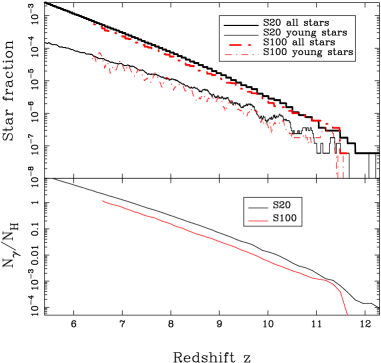
Figure 2: Top panel: Evolution of the fraction of baryonic mass locked into stars. Stars are considered young for the first 5-20 Myr. Bottom panel: Number of emitted photons per hydrogen atom.

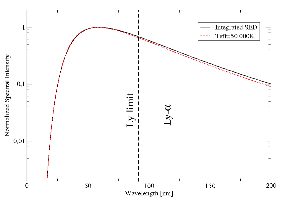
Figure 3: Normalized spectral intensity as a function of wavelength.

3.2.2 Post-treatment of the dynamical simulations: the issue of gas heating

We use the snapshots of the dynamical runs as inputs for the radiative transfer simulation. Consequently, there is no feedback on the dynamics from the radiative heating of the gas. This has two opposite effects. First it slows down to some extent the propagation of the ionization fronts since the high gas pressure inside the Strömgren sphere is not effective. Second the source formation is not quenched by radiative feedback : stronger sources speed up the ionization front propagation. The net result of these two effects is unclear. In view of other important uncertainties, like the source modeling, the feedback of radiative transfer on the dynamics is neglected.

The second consequence of running the radiative transfer simulation in post-treatment of the dynamical simulation is that dynamical effects on the temperature of the gas due to shock heating are not included in the radiative transfer simulation.

Shock heating is a sensitive issue since it directly affects the $21$ cm signal, possibly transforming absorption into emission by raising the gas temperature above the CMB temperature. For example, mini-halos with masses between $10^{4}$ to $10^{8}$ M_⊙ form very early during the EoR and are dense and warm enough from shock heating during virialization to emit $21$ cm radiation. Iliev et al. (Iliev02 (2002)) and Shapiro et al. (Shapiro06 (2006)) show that the emission of mini-halos can dominate the $21$ cm signal prior to the onset of Ly-$\alpha$ coupling. Furlanetto and Oh (2006c ), however, find that the contribution of diffuse regions dominates later on. The simulations presented here only marginally resolve the most massive of these mini-halos in the best case (S20 simulation), and we chose not to try to include them as subgrid physics. But we should keep in mind that shock heating both below and above our scale resolution may affect the $21$ cm signal, as long as it occurs in neutral regions (mini-halos, filaments).

The adiabatic cooling of the gas by dynamical expansion in low density regions is also an important factor responsible for the possible strong absorption features in the $21\,\rm{cm}$ maps : we can take it into account easily during the post treatment. We use the fact that, below $T=10^{4}$ K (always true in neutral, $21\,\rm{cm}$ emitting regions), the cooling rate of the primordial gas is negligible, and shock heating is limited in the low density diffuse regions of the IGM. Consequently, we approximate the thermal evolution of the gas in the dynamical simulation as adiabatic. We compute the variation of internal energy of a particle due to expansion or contraction between two consecutive snapshots from the variation of the density :

$$\bigtriangleup u=u_{2}-u_{1}=u_{1}\left(\left(\frac{\rho_{2}}{\rho_{1}}\right)^{\gamma-1}-1\right),$$ (6)

where $u$ is the internal energy and $\rho$ is the gas density.

However, if the variation in density between two snapshots is large, applying it all at once results in numerical instabilities. This happens when particles pass through or collapse into a halo. To avoid this, the density is interpolated gradually between two snapshots.

The other cooling and heating processes are then included self-consistently in the radiative transfer simulation. We use the cooling-heating rates in Cen (Cen92 (1992)), and a minimum gas temperature of $1$K.

3.2.3 Source modeling

In this work we consider only stellar sources and do not study the influence of X-ray sources. The decline of the quasar luminosity function at redshift $z>3$ suggests that stars were the dominant source of ionizing photons during the EoR (Shapiro & Giroux Shapiro87 (1987), or Faucher-Giguère et al. Faucher-Giguere08 (2008) for recent observational evidence). However, even in small quantities, X-ray sources have the potential to affect the $21$ cm signal by heating the IGM. Indeed X-ray photons can have a mean free path of several $100\,\rm{Mpc}$ through neutral hydrogen during the EoR: they propagate through the ionization front out to the neutral regions. Using a homogeneous model Glover & Brand (Glover03 (2003)) find that a modest number of X-ray sources can raise the temperature of the IGM by several tens of K. Moreover, Pritchard & Furlanetto (Pritchard07 (2007)) show that the heating by X-rays is actually not homogenous: it produces fluctuations in the gas temperature which leave their own imprint on the $21$ cm power spectrum. In this work, however, we want to focus on the specific influence of Ly-$\alpha$ pumping. X-ray sources will be included in a future work.

All baryon particles have the same mass : $7.6\times 10^{6}M_{\odot}$ (resp. $9.5\times 10^{8}M_{\odot}$) for the S20 (resp. S100) simulation. Accordingly, one star particle corresponds in fact to a star cluster or a dwarf galaxy so an IMF has to be assumed. We choose a Salpeter IMF, with masses in the range 1M_⊙ - 100M_⊙. Then we compute the total luminosity and spectral energy distribution (SED) for one star particle by integrating over the IMF. We use the table in Aller (Aller82 (1982)) to obtain the radius and effective temperature of stars as a function of mass. The total ionizing luminosity (tab. 2) of a star particle yields one or two photons per hydrogen atom at z=6.5 (Fig. 2). The resulting SED is plotted in Fig. 3. It can be seen that it differs very little from a blackbody spectrum with $5\times 10^{4}\tiny$ K effective temperature. Therefore our source model is roughly intermediate between PopII and PopIII stars.

simulations	$L_{tot}[erg/s]$	$f_{esc}$
S20	$4.60\times 10^{43}$	$0.08$
S100	$5.75\times 10^{45}$	$0.05$

Table 2: The total ionizing luminosity of a star particle and escape fraction of simulations

3.2.4 Calibrating the global ionization history

Before making a global calibration using the escape fraction, we need to consider the effect of the time evolution of the stellar population within one source particle. Massive stars contribute the most to the ionizing luminosity of the source, but live for a shorter time. We use a simple model : when a new source particle is created, we assign it a random lifetime between 5Myr and 20Myr as a source of ionizing photons. The randomization is useful because we obtain new sources only with each new dynamical snapshot; a fixed lifetime for all sources and a discreetly evolving number of sources with each new snapshot would produce distinct steps in the average ionizing flux. Globally, the average lifetime of the source is degenerate with the escape fraction as far as ionization history calibration is concerned, however, it allows us to account for the signature of local starbursts (in time and space) followed by quiescence. We plot the effect of considering a finite lifetime for the ionizing source on the star fraction history in Fig. 2. It can be seen that the young, ionizing star fraction fluctuates more strongly at high redshifts than the global star fraction. A combination of local starbursts followed by star formation quenching and insufficient mass resolution may be responsible for this effect.

By trial and error, we calibrated the escape fraction (tab. 2) so that reionization is complete, at about $z\sim 6$.

3.3 Lyman-$\alpha$ transfer

We run the Lyman-$\alpha$ simulations as a further post-treatment of the reionization simulations. The time interval between two snapshots is typically $10$ Myr at $z\sim 9$, during which the ionization fronts travel a few hundred comoving kpc at most. We consider that this time interval is small enough to permit a de facto interpolation of the quantities relevant for Lyman-$\alpha$ transfer : gas density and ionization state.

Potentially, Lyman series photons can heat up the gas (see references in Semelin et al. Semelin07 (2007)). But heating occurs only at low temperatures ($\sim 10$ K), where the gas pressure is insignificant. Consequently, the feedback of Lyman-$\alpha$ photons on the dynamics is negligible. However, in models with soft source spectra, where the efficient heating of low density neutral regions by X-ray photons is absent, one consequence of including the heating by Lyman-$\alpha$ photons is to increase moderately the temperature in the coolest regions. We implemented a local Lyman-$\alpha$ heating using the following formula, derived from Eq. $47$ and Fig. $3$ in Furlanetto & Pritchard (2006b ) :

$${dT_{K}\over dt}={0.8\over T_{K}^{1/3}}\,{x_{\alpha}\over S_{\alpha}}\,{10\over 1+z}\,H(z)\quad\mathrm{with}\quad S_{\alpha}\sim\left(1-{0.7\over\sqrt{T_{K}}}\right)$$ (7)

We checked that when the $21\,\rm{cm}$ signal is in absorption with an intensity in the $300\,\rm{mK}$ range, i. e. where the gas temperature is a few K, this small amount of heating can reduce the signal intensity by up to $100\,\rm{mK}$.

Photons are emitted at frequencies between Ly-$\alpha$ and Ly-$\beta$. The spectrum and luminosity of the sources are computed with the method described in section 2.2.3 for the ionizing continuum. In principle higher Lyman series photons also contribute. Indeed as soon as a photon emitted in the continuum hits an atom in a resonant upper Lyman line, it cascades locally down the levels and is transformed into a local Ly-$\alpha$ photon. These higher Lyman line photons are more concentrated around the sources since they need a smaller redshift before they resonate with a line (see e.g. Naoz & Barkana Naoz08 (2008)). Overall, including the upper Lyman line photons would increase the number of Ly-$\alpha$ photons by a factor of less than 2. From the results of the simulations we estimate that this could shift the history of the average Ly-$\alpha$ coupling by $\Delta z=0.3$. It would also add some limited amount of power in the fluctuations. In this work we include only the Ly-$\alpha$ line. Upper Lyman series lines will be included in a future work.

In the simulations, a fiducial number of $n_{\rm{ph}}=10^{7}$ photons is used between two dynamical snapshots. As the time interval between snapshots and the total source intensity varies, the physical content of the photons also varies. The value of $n_{\rm{ph}}=10^{7}$, dictated by the CPU cost of the simulations, is a lower limit for statistical significance : indeed, with our current grid resolution of less than 12 particles per cell, about $10\%$ of the cells do not receive any photons between two snapshots. These cells are small and are mostly located in moderate density filaments and low flux environments, far from the sources. They are properly averaged with some of their neighbors when the fixed-grid maps are computed. To assess the impact of this limited sampling we also ran a simulation with $6\,\times 10^{7}$ photons between two snapshots down to $z=9.5$ for the $20$ h^-1 Mpc box. In this case the fraction of unsampled cells drops to $\sim 1\%$. It is only when maps are drawn with thin slices, $\sim 200\,h^{-1}\,\rm{kpc}$, that a difference can be seen.

3.4 Physics of the $21\,\rm{cm}$ emission

To compute the differential brightness temperature of the $21\,\rm{cm}$ emission in the optically thin limit of the $21\,\rm{cm}$ line, we use the formula :

$$\delta T_{b}=28.1\,\,{\mathrm{mK}}\,\,x_{\mathrm{HI}}\,\,(1+\delta)\left({1+z\over 10}\right)^{1\over 2}\,\,{T_{S}-T_{\mathrm{CMB}}\over T_{S}}$$

$$\hskip 42.67912pt\times\left({\Omega_{b}\over 0.042}{h\over 0.73}\right)\left(0.24\over\Omega_{m}\right)^{1\over 2}\left({1-Y_{p}\over 1-0.248}\right)\,,$$ (8)

where $\delta$ is the local overdensity at redshift $z$, $x_{\mathrm{HI}}$ the neutral hydrogen fraction, $T_{S}$ the neutral hydrogen spin temperature, $T_{\mathrm{CMB}}$ the CMB radiation blackbody temperature at redshift $z$ and $\Omega_{b}$, $\Omega_{m}$, $h$ and $Y_{p}$ are the usual cosmological parameters. In this formula, the contribution from the proper velocity gradients have been neglected (Barkana & Loeb 2005a ). Mellema et al. (2006b ) include this effect in computing $21$ cm line of sight spectra. Analytic (McQuinn et al. McQuinn06 (2006)) and semi-numerical models (Mesinger & Furlanetto Mesinger07 (2007)) find that the contribution of proper velocity gradients to the $21$ cm power spectrum is important only at $\langle x_{\mathrm{HI}}\rangle<0.5$ on scales smaller than the effective ionization bubble size. Since previous simulations did not include a proper treatment of the Ly-$\alpha$ pumping which is especially important during the early phase of reionization, it was not relevant to include the effect of proper velocity gradients. In this work, we include a full modeling of the Ly-$\alpha$ pumping. In a separate paper, the effect of proper velocity gradients will be studied.

The spin temperature of hydrogen $T_{S}$ is coupled to the CMB temperature $T_{\mathrm{CMB}}$ by Thomson scattering of CMB photons, and to the kinetic temperature of the gas $T_{K}$ by collisions and Ly-$\alpha$ pumping. As a result, the spin temperature can be written (Furlanetto et al, 2006a) :

$$T_{S}^{-1}={T_{\mathrm{CMB}}^{-1}+x_{c}T_{K}^{-1}+x_{\alpha}T_{C}^{-1}\over 1+x_{c}+x_{\alpha}}\quad\mathrm{with}\quad T_{C}\simeq T_{K}\,,$$ (9)

and

$$x_{\alpha}={4P_{\alpha}T_{\star}\over 27A_{10}T_{\mathrm{CMB}}},\quad x_{c}={T_{\star}\over A_{10}T_{\mathrm{CMB}}}(C_{H}+C_{p}+C_{n}),\,$$ (10)

where $T_{\star}={h\nu_{0}\over k_{B}}=0.068\,\rm{K}$ ($\nu_{0}=1420\,\rm{MHz}$), $A_{10}=2.85\times 10^{-15}s^{-1}$ is the spontaneous emission factor of the $21\,\rm{cm}$ transition, $P_{\alpha}$ is the number of scatterings of Ly-$\alpha$ photons per atom per second, and $C_{H}$, $C_{p}$ and $C_{e}$ are the de-excitation rates due to collisions with neutral atoms, protons and electrons. For the de-excitation rates we use the fitting formula given by Liszt (Liszt01 (2001)) and Kuhlen et al. (Kuhlen06 (2006)). The coupling coefficients $x_{\alpha}$ and $x_{c}$ are computed for each gas particle from the simulation data. The final output is the value of the brightness temperature for each particle in each snapshot.

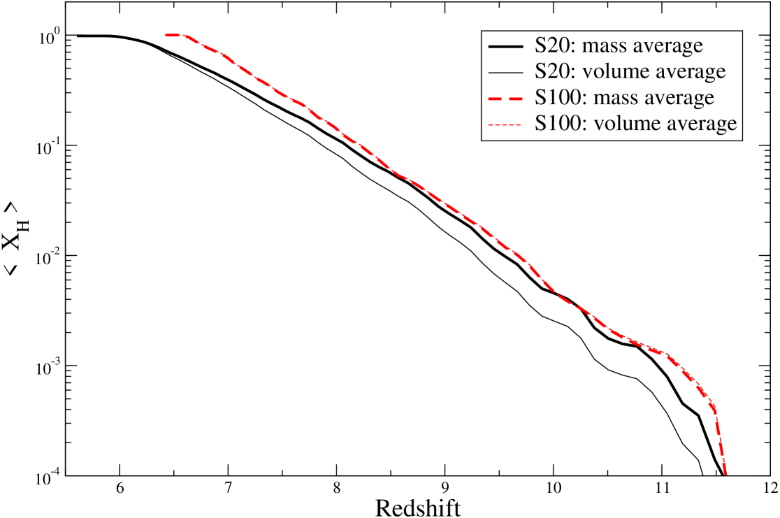
Figure 4: Mass weighted and volume weighted averaged ionization fraction.

4 Analysis

We will focus our analysis on two aspects.

First, by comparing our two simulations, we will evaluate the effect of numerical resolution and box size. Numerical resolution truncates the physics at small scales : this mainly modifies the reionization history and geometry by removing small, dense structures with high recombination rates. The limited box size, on the other hand, truncates large scales and dampens the $21\,\rm{cm}$ brightness temperature power spectrum on corresponding wavenumbers.

The second axis of our analysis is to measure the effect of including an accurate treatment of the Wouthuysen-Field effect in computing the brightness temperature.

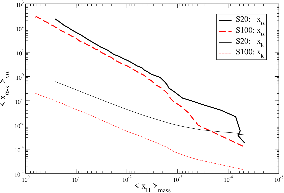
Figure 5: Evolution of the volume averaged Lyman-$\alpha$ and collisional coupling coefficients as functions of the average ionization fraction for both simulations (see main text for a definition of the coefficients).

4.1 Evolution of sky-averaged quantities

4.1.1 Ionization fraction

The simplest way to characterize the global history of reionization is to compute the average ionization fraction as a function of redshift. The mass weighted ($\langle x_{H}\rangle_{\rm{mass}}$) and volume weighted ($\langle x_{H}\rangle_{\rm{vol}}$) average ionization fractions are shown in Fig. 4 for both simulations. For the volume (resp. mass) average we use the volume occupied by each particle derived from the SPH smoothing length (resp. the mass of each particle) as weights in the averaging procedure. The main feature of this plot is that the mass weighted averages are similar for the two simulations while the volume weighted averages differ. Indeed, the star formation histories of the two simulations were calibrated to produce the same number of ionizing photons at any redshift. As long as recombination is negligible, this should produce identical mass weighted ionization fractions. It can be checked in Fig. 4 that below redshift $\sim 8$ recombination becomes efficient in the S20 simulation, which contains denser small-scale structures due to higher resolution, and the mass weighted ionization fraction drops below its S100 counterpart.

The volume weighted ionization fractions differ at all redshifts between the two simulations, because highly ionized regions of identical mass, close to the sources, are denser and occupy a smaller volume in the more resolved S20 simulation. McQuinn et al. (McQuinn06 (2006)) advocate the use of the volume-averaged ionization fraction as an evolution variable instead of redshift. Indeed, depending on arbitrary choices (all consistent with current observational constraints) for the source formation history and source nature, reionization can begin at $z=12$, $15$ or $20$ and proceed differently. However, for a fixed average ionization fraction, McQuinn et al. (McQuinn06 (2006)) show that the brightness temperature power spectrum depends weakly on the redshift at which this ionization fraction is achieved. This is true if a modification of the source formation efficiency is the main cause of the change in redshift for a fixed ionization fraction. If the change is caused by using a different source spectrum, or modifying the gas sub-grid physics (e.g. an inhomogenous clumping factor), this may not be true anymore. We believe that the averaged ionization factor is indeed a more relevant measure of the evolution of reionization than redshift and we adopt their point of view. However, instead of the volume averaged ionization fraction, which is well suited to comparing different models with the same underlying gas density field, we will use the mass averaged ionization fraction which is better suited for the comparison of simulations with different mass resolution. While the mass averaged ionization fraction is a suitable quantity to track the progression of reionization, a volume average is more relevant to compute such observable quantities as the $21\,\rm{cm}$ brightness temperature. Consequently, all quantities other than the ionization fraction will be volume averaged.

We also computed the Thomson optical depth from the two simulations ignoring the presence of helium. The values are $\tau=0.060$ and $\tau=0.063$ for S20 and S100 simulations respectively, i.e. within $1\sigma$ of the WMAP3 value $\tau=0.0089\pm 0.030$ (see Spergel et al. Spergel07 (2007)).

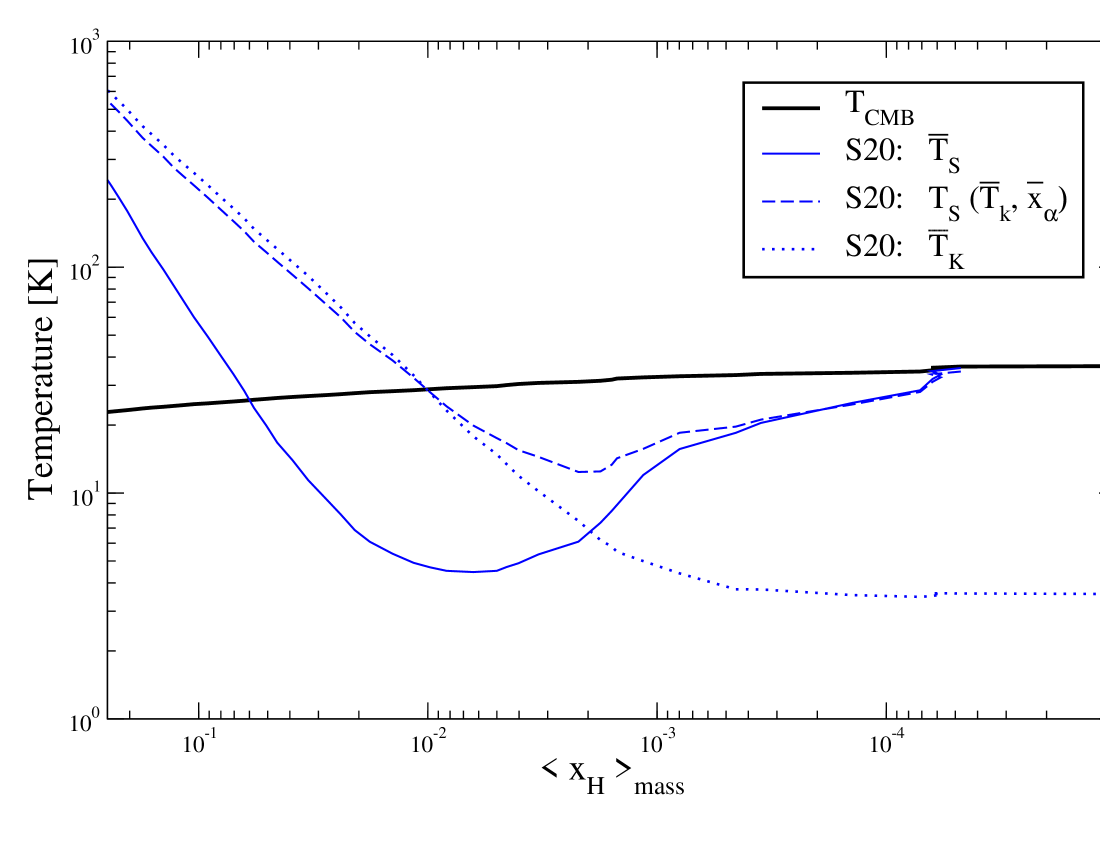
Figure 6: Evolution of the neutral hydrogen spin temperature as a function of the average ionization fraction. The average is computed either directly from the particle spin temperatures or from the volume averaged values of $T_{K}$ and $x_{\alpha}$. The CMB temperature and volume averaged kinetic temperature are plotted for comparison.

4.1.2 Spin temperature coupling coefficients

The spin temperature of neutral hydrogen, $T_{S}$, is defined by Eq. $7$ and depends on two coupling coefficients, $x_{\alpha}$ for the Wouthuysen-Field coupling and $x_{k}$ for collisional coupling. Until now, $x_{\alpha}$ has never been computed consistently in simulations of the $21\,\rm{cm}$ emission. While $x_{\alpha}$ itself contains fluctuations which contribute to the power spectrum of the $21\,\rm{cm}$ signal, we study first the evolution of the average value of the coefficients which tells us at which stage in the reionization history the spin temperature can be considered fully coupled to the kinetic temperature of the gas. The evolution of the volume averaged coefficients $\langle x_{\alpha}\rangle_{\rm{vol}}$ and $\langle x_{k}\rangle_{\rm{vol}}$ is shown in Fig. 5, as a function of $\langle x_{H}\rangle_{\rm{mass}}$. The first conclusion from Fig. 5 is that $x_{k}$ is negligible compared to $x_{\alpha}$ except in the very early phase ($\langle x_{H}\rangle_{\rm{mass}}\sim 10^{-4}$) for the S20 simulation. Logically, the S20 simulation, producing denser structures, has a higher $x_{k}$ (indeed $C_{H}$, $C_{p}$ and $C_{e}$ in Eq. $8$ depend on the density). With a better mass resolution and even denser structures than in the S20 simulation, $x_{k}$ would still increase, and the ionization fraction when $x_{\alpha}$ starts to dominate would also increase. The second piece of information that can be derived is the magnitude of the error made by applying the usual assumption $x_{\alpha}=+\infty$. When $x_{\alpha}>10$, the error made on $\delta T_{b}$ by assuming $x_{\alpha}=+\infty$ is smaller than $\sim 10\%$. This corresponds to $\langle x_{H}\rangle_{\rm{mass}}>0.02$ for the S20 simulation and $\langle x_{H}\rangle_{\rm{mass}}>0.04$ for the S100 simulation. It may appear that the full coupling occurs very early on. Let us emphasize, however, that in this early phase there is a strong absorption signal (with our choice of source model) compared with the weaker emission signal observed later on. In a source model with a harder spectrum (to be studied in a future paper) we would have a weaker absorption signal. If the sources are still stars ( e.g. using a more top-heavy IMF) the full coupling would also occur at a larger average ionization fraction since the ratio of ionizing to Lyman-alpha photons would be larger.

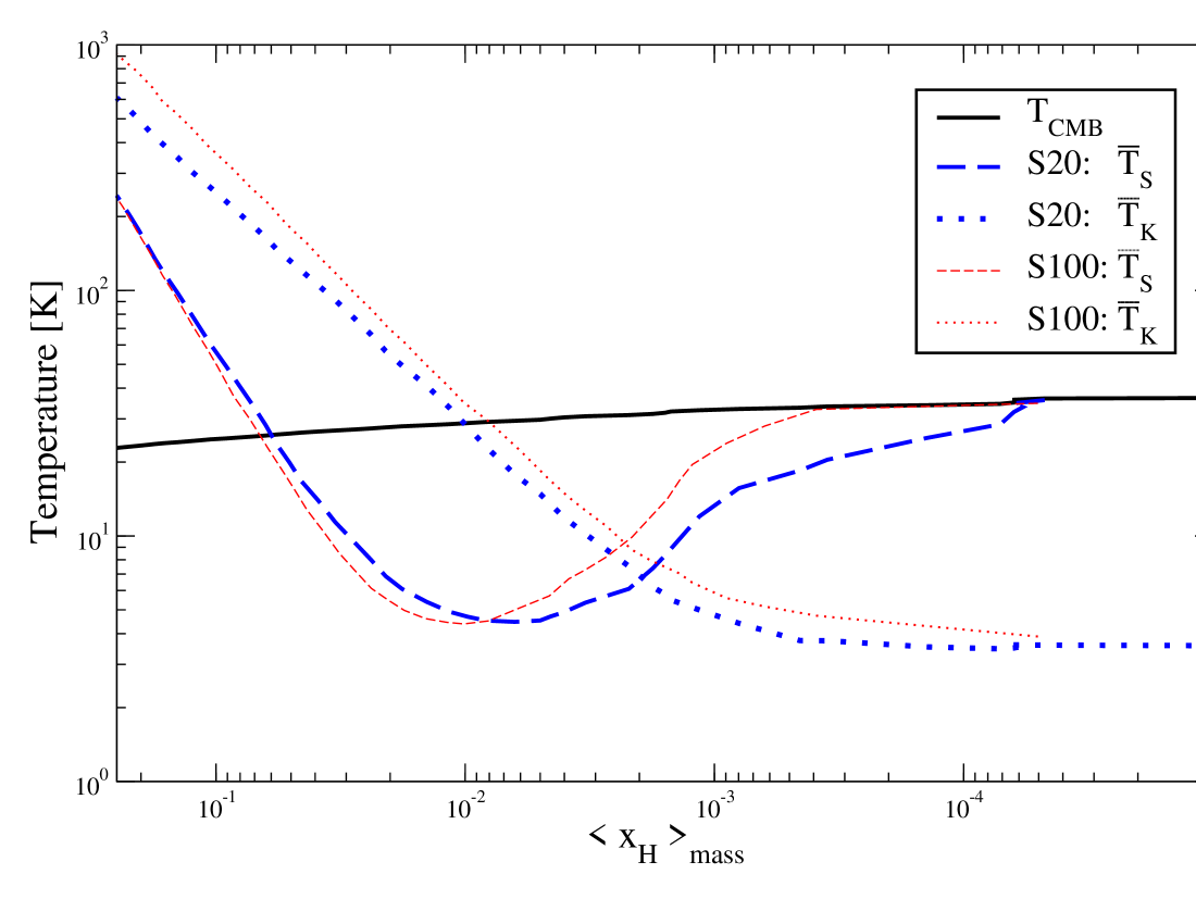
Figure 7: The evolution of the volume averaged spin temperature, kinetic temperature, and CMB temperature is plotted as a function of the average ionization fraction. The quantities are plotted for both box sizes.

4.1.3 Spin temperature

Fig. 6 displays the average spin temperature for the S20 simulation, with the average computed in two different ways. First the spin temperature is computed using the volume averaged quantities $\langle T_{k}\rangle_{\rm{vol}}$, $\langle x_{\alpha}\rangle_{\rm{vol}}$ (and $\langle x_{k}\rangle_{\rm{vol}}$), following Furlanetto et al. (2006a ) and Gnedin & Shaver (Gnedin04 (2004)). This quantity is denoted $T_{S}(\bar{T}_{K},\bar{x}_{\alpha})$. Then the more relevant value, $\bar{T}_{S}$, is computed, as the direct volume average on the particles of the spin temperature, i.e. $\bar{T}_{S}=\langle T_{S}\rangle_{\rm{vol}}$. Fig. 6 shows that there is a large difference between the two definitions. This is mainly due to the fact that the spin temperature is computed through the weighted average of inverse temperatures (Eq. $7$). This large difference propagates to the average brightness temperature. Consequently we strongly advocate replacing the Furlanetto et al. average traditionally used to define the emission and absorption regimes by the more relevant direct average of the spin/brightness temperature. Of course this is easily done only for simulations. Let us mention that with the direct average, the spin temperature remains below the CMB temperature at lower $z$.

Fig. 7 compares the direct average of the particle spin temperature in the two simulations : the results are quite similar. The main difference is that the spin temperature starts to decouple from the CMB temperature later in the S100 simulation. Indeed, we use periodic boundary conditions in the simulations. Thus the Lyman-$\alpha$ sources are more homogeneously distributed in the $20\,h^{-1}\,\rm{Mpc}$ box, which lacks large scale modes, than in the $100\,h^{-1}\,\rm{Mpc}$ box (Barkana & Loeb 2005b ). In the $100\,h^{-1}\,\rm{Mpc}$ box, large void regions receive little Lyman-$\alpha$ flux. There, the spin temperature remains coupled to the CMB at lower redshifts.

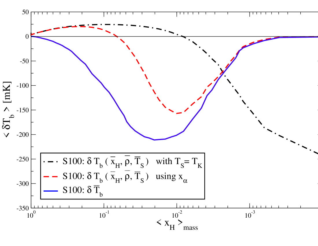
Figure 8: Evolution of the average differential brightness temperature for the S100 simulation. The average is computed in three different ways (see main text and legend). The blue curve is the most relevant direct average of the particle brightness temperature.

4.1.4 Differential brightness temperature

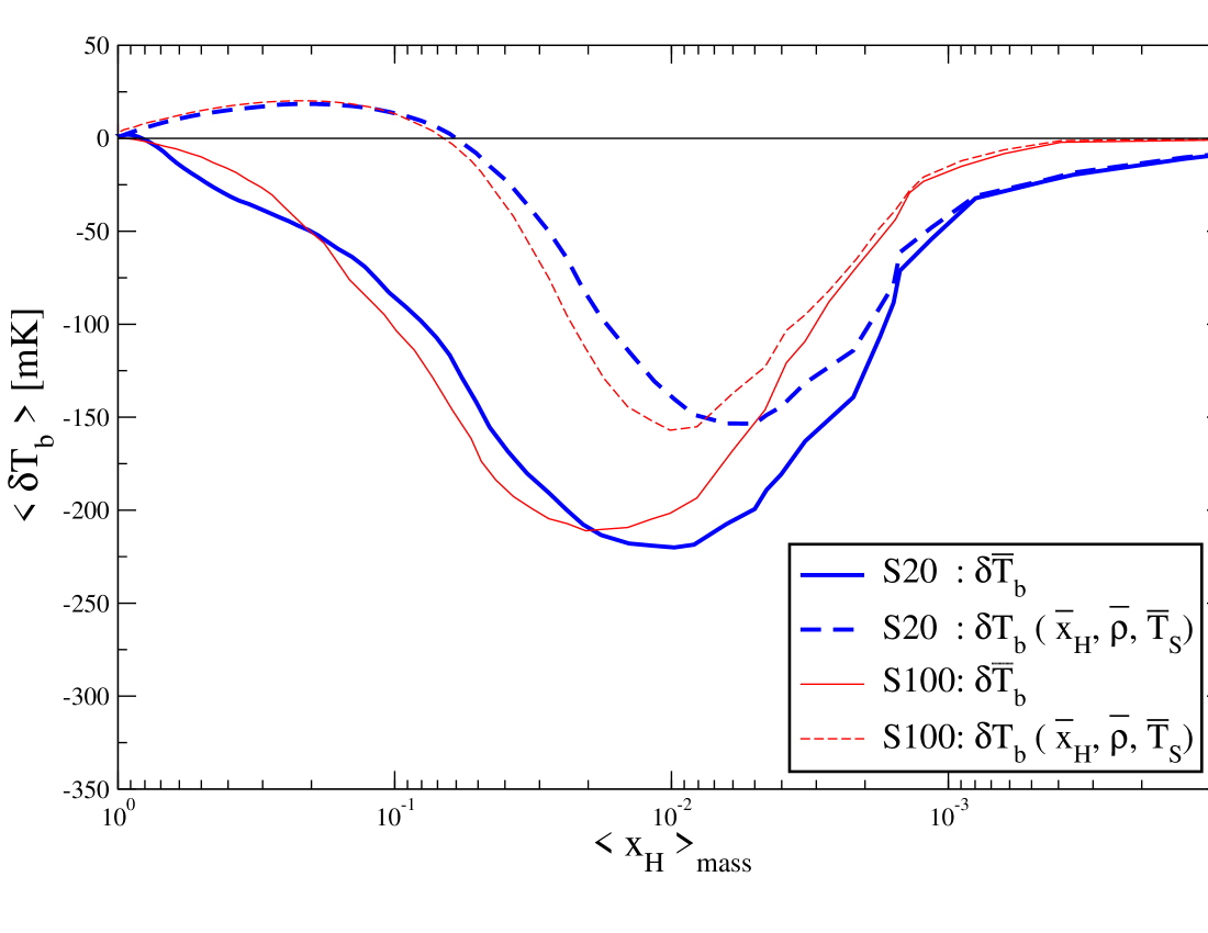
Figure 9: Comparison of the evolution of the average differential brightness temperature for the two box sizes. The average is computed in two different ways (see main text).

The differential brightness temperature is plotted in Fig. 8 for the S100 simulation. The average is computed in three different ways : $\delta T_{b}(\bar{x}_{H},\bar{\rho},\bar{T}_{S})$ with $T_{S}=T_{K}$ for each particle, $\delta T_{b}(\bar{x}_{H},\bar{\rho},\bar{T}_{S})$ computing $T_{S}$ for each particle using $x_{\alpha}$, and $\bar{\delta T}_{b}$, using the same notations as for the spin temperature. In all these definitions we use a volume weighted average. The first definition uses the common $T_{S}=T_{K}$ assumption : as can be seen in the plot, it fails at early times when the coupling is weak. The second definition (equivalent to Furlanetto et al. 2006a ) shows an emission and an absorption regime. However, with the more realistic third definition, $\bar{\delta T}_{b}$, the emission regime disappears completely. Indeed, absorption region have a strong signal which dominated over the weak, $\sim 25\,\rm{mK}$ signal of the emitting regions. Of course, if X-ray sources were included, the cold neutral IGM would be pre-heated and the absorption regions contribution would shrink much faster : $\bar{\delta T}_{b}$ would show an emission regime and the absorption regime would be weaker. Including shock heating would go in the same direction although the magnitude of the change would be less homogenous and is more difficult to estimate.

To assess the effect of resolution and box size, we plot in Fig. 9 the direct $\bar{\delta T}_{b}$ and $\delta T_{b}(\bar{x}_{H},\bar{\rho},\bar{T}_{S})$ for both simulations. The overall behaviour is similar. In the S20 simulation the minimum of $\bar{\delta T}_{b}$ occurs at a $1\%$ average ionization fraction compared to a $2\%$ ionization fraction for the S100 simulation. This small difference is due in part to the slightly smaller coupling of the S100 simulation at equal ionization fraction. The values of the minimum $\bar{\delta T}_{b}$ are not very different either. We expect to find resolution effects and box size effects in the power spectra.

We have presented these average values to compare with previous studies. However, much information is erased when considering average quantities, which makes their interpretation of limited scope. We proceed now to present maps of the different quantities.

4.2 Maps

4.2.1 Ionization fraction

Maps of the ionization fraction of hydrogen are presented in Fig. 10 for both box sizes at a redshift when $\langle x_{\alpha}\rangle_{\rm{vol}}=1$, which we will call the Wouthuysen-Field coupling redshift (hereafter WFCR), and at a redshift when $\langle x_{H}\rangle_{\rm{mass}}=0.5$, which we will call the half reionization redshift (HRR). We can see that the WFCR correspond to an early stage in the reionization history. The maps are presented for two different slice thicknesses : $2\,h^{-1}\,\rm{Mpc}$ and $200\,h^{-1}\,\rm{kpc}$. The $2\,h^{-1}\,\rm{Mpc}$ slice corresponds to a bandwidth $\delta\nu\sim 0.15$ MHz at a redshift between $6$ and $10$, an acceptable value for SKA. The $200$ h^-1 kpc slice is plotted to give a feeling of how much power would be added at small scales by using narrower bandwidth : indeed, sharper ionization fronts are found in this case. Also as expected the S100 maps show coherent structures on scales up to $50\,h^{-1}\,\rm{Mpc}$ which cannot be accounted for in the S20 maps.

Usual effect of a lower mass resolution (S100 vs S20) is to delay reionization. Indeed small mass halos form first and make a large contribution to the ionizing photon budget at early times (see Iliev et al. Iliev07 (2007)). In our treatment, the delay is removed because we calibrated the source formation history of the S100 simulation on the S20 simulation by boosting the formation efficiency. However, this procedure can only account for unresolved halos located within more massive, resolved, proto-halos. The contribution from unresolved halos located in comparatively underdense regions could modify the morphology of the ionization maps during the early reionization history.

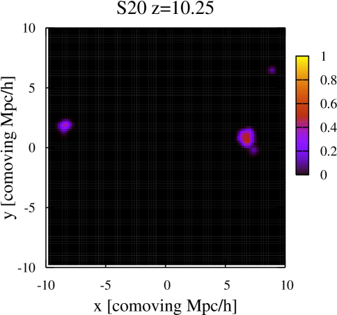
$2\,\,\,\mathrm{Mpc/h}$ (comoving) slice

         

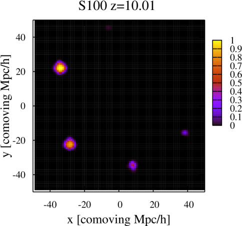
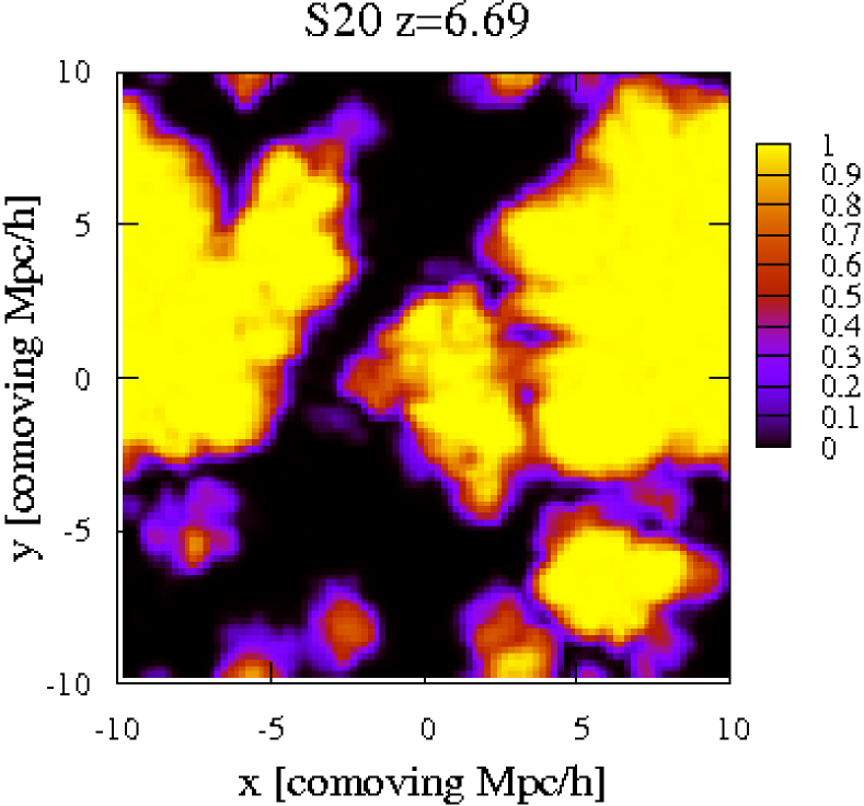
$2\,\,\,\mathrm{Mpc/h}$ (comoving) slice

         

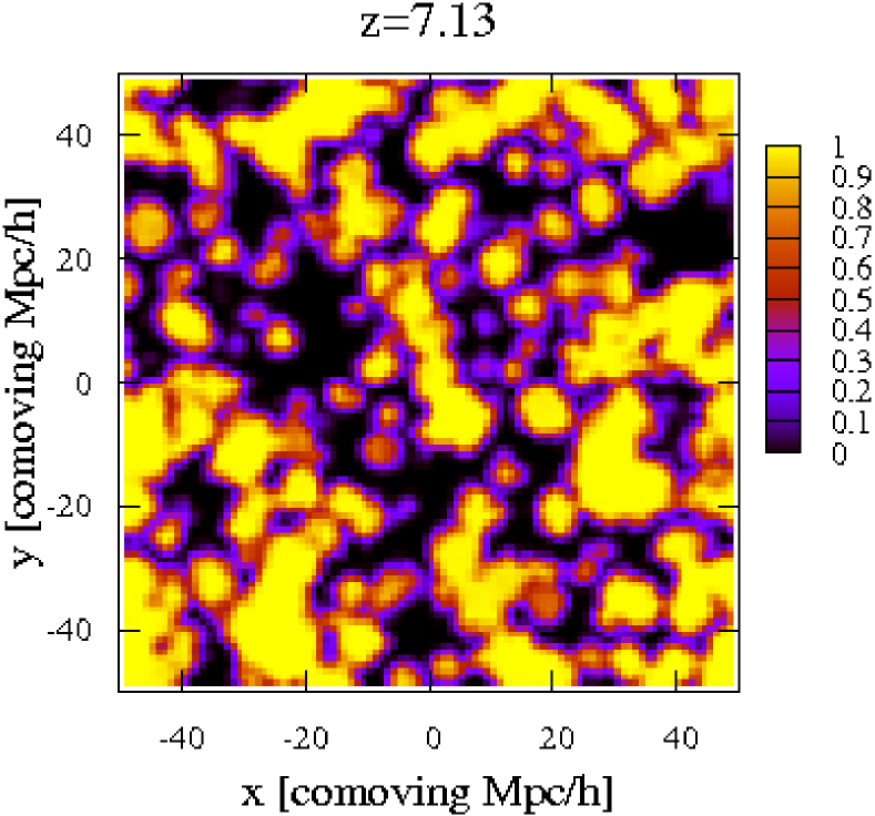
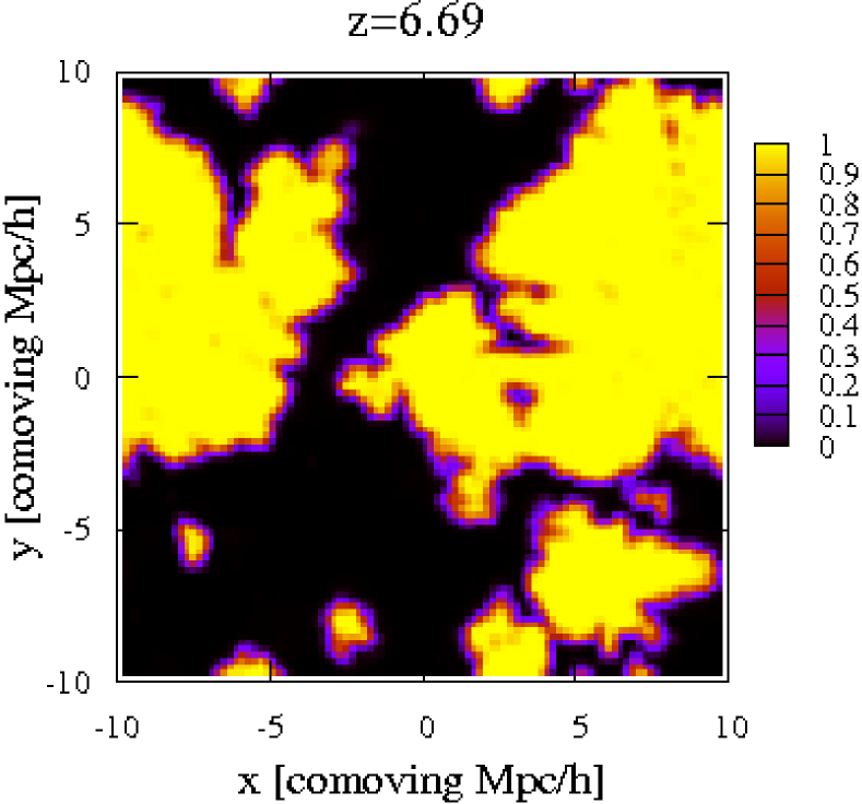
$200\,\,\,\mathrm{kpc/h}$ (comoving) slice

         

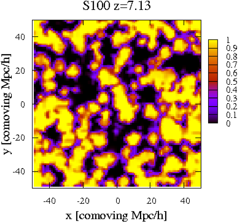
Figure 10: Maps of the ionization fraction for the two simulations (right and left) at two different stages of reionization (above and below line), the WFCR and the HRR (see text for definition) and for two slice thicknesses (as labeled). The color scale is a linear function of the ionization fraction.

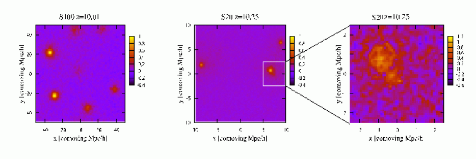
Figure 11: Maps of the $x_{\alpha}$ coupling coefficient. We use a logarithmic color scale, and choose the redshift in each simulation (S20 and S100) such that $\langle x_{\alpha}\rangle=1$ (10.25 for S20 and 10.01 for S100). The thickness of the slice is $2\,h^{-1}\,\rm{Mpc}$ for the two panels on the left and $100$ h^-1.kpc for the right panel.

4.2.2 Lyman-$\alpha$ coupling

The influence of including a proper treatment of the Wouthuysen-Field effect on the $21\,\rm{cm}$ signal is twofold. First, it simply modifies the intensity of the signal, especially in the regions seen in absorption. This will be obvious in the brightness temperature maps shown in section 4.2.3. The second effect is to introduce a new source of fluctuations in the signal, associated with the fluctuations in the local Ly-$\alpha$ flux. Fig. 11 presents maps of the $x_{\alpha}$ coefficient for both simulations at the WFCR. Around the WFCR, the additional fluctuations to the brightness temperature are expected to be maximal. On a large scale, the maps boil down to strong coupling regions around sources, superimposed on a uniform weak coupling background. The signature of the added brightness temperature fluctuations will be based on the typical sizes of the strong coupling regions and on the clustering and Poisson noise in the source distribution. Keeping this in mind, it is interesting to notice that the strong coupling regions appear to be much smaller, $\sim 2\,h^{-1}\,\rm{Mpc}$, in the S20 simulation than in the S100 simulation where they extend over $\sim 10\,h^{-1}\,\rm{Mpc}$. To understand this let us remember that we apply periodic boundary conditions to the radiative transfer code. As a result, any point in the S20 simulation is surrounded by a rather homogeneous distribution of sources, with the closest source at most $\sim 10\,h^{-1}\,\rm{Mpc}$ away. This dampens the fluctuations in the Ly-$\alpha$ flux and washes out the outer parts of the strong coupling regions. As a result, we expect to find more power at large scales in the added brightness temperature fluctuations in the S100 simulation than in the S20 simulation.

The zoom on the source in the S20 simulation shows that the apparent spherical symmetry of the strong coupling regions breaks down at small scales. Semelin et al. (Semelin07 (2007)) have shown that substantial asymmetry can be expected if the density field of the gas is not homogeneous (e.g. presence of filaments). Let us notice, however, that the slice thickness for the zoom is $100$ h^-1 kpc, while it is $2\,h^{-1}\,\rm{Mpc}$ for the other maps. With such a thin slice the noise in the $x_{\alpha}$ evaluation (resulting of the finite number of photons used in the Monte Carlo scheme) is not smoothed out at all. Any structure outside the main strong coupling region is mostly noise (visible on the color version only). If structures exist in the $x_{\alpha}$ maps at scales smaller than $1\,h^{-1}\,\rm{Mpc}$ and with an amplitude of less than a factor of $3$ above or below the background, we will miss them in the noise or smooth them out. From a theoretical point of view it would be interesting (but very costly) to produce maps with a lower noise level. However, from a practical point a view, these scales are below the projected resolution of SKA.

4.2.3 Brightness temperature maps

The most common (and most drastic) approximation used to compute the brightness temperature is $T_{S}\gg T_{CMB}$ (case 1). In this approximation no absorption region can exist. The second approach is to assume full Lyman-$\alpha$ coupling ($x_{\alpha}=\infty$) (case 2). The third approach, the one used in this paper, is to compute self-consistently the local values of $x_{\alpha}$ and derive accordingly the local values of $T_{S}$ and $T_{b}$ (case 3). We plot maps of the differential brightness temperature for all three cases and for both simulation boxes at the WFCR in the 6 top panels of Fig. 12. The thickness of the slice is $2\,h^{-1}\,\rm{Mpc}$ . At this early redshift, when the two first approximations are hardly reliable, the differences are striking. Not surprisingly case 1 fails completely : it is not tailored to handle absorption regions and predicts only emission. More interesting, but also expected, case 2 overpredicts the strength of the absorption compared to case 3 ($300\,\rm{mK}$ instead of $200\,\rm{mK}$) by assuming full Wouthuysen-Field coupling. We used the same color scale for all maps to emphasize these differences. The strong absorption signal observed in cases 2 and 3 is the consequence of our choice of rather soft-spectrum sources. The neutral IGM undergoes very little pre-heating by UV and X rays. Let us emphasize that the strength of the absorption signal is very sensitive to the thermal modeling of the gas when $T_{K}\ll T_{CMB}$, which is not uncommon at this redshift with our choice of sources. Indeed, the included Ly-$\alpha$ heating, although very weak (at most a few K over the EoR), decreases the strength of the absorption signal by $50$ to $100\,\rm{mK}$. If even a small fraction of hard-spectrum sources was included, the absorption strength would decrease and turn to emission at later redshifts .

Case 1 : $T_{S}\gg T_{CMB}$Case 2 : $T_{S}=T_{K}$Case 3 : $T_{S}(x_{\alpha})$

   

   

   

   

   

   

   

   

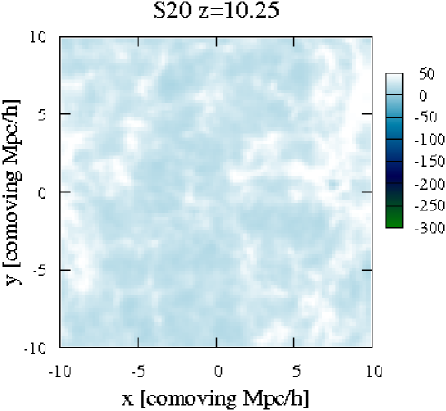
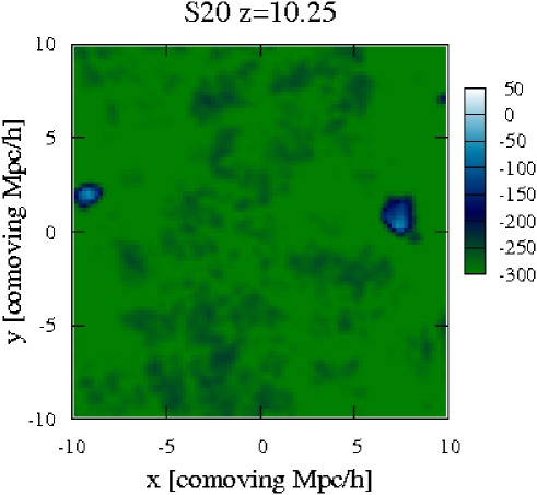
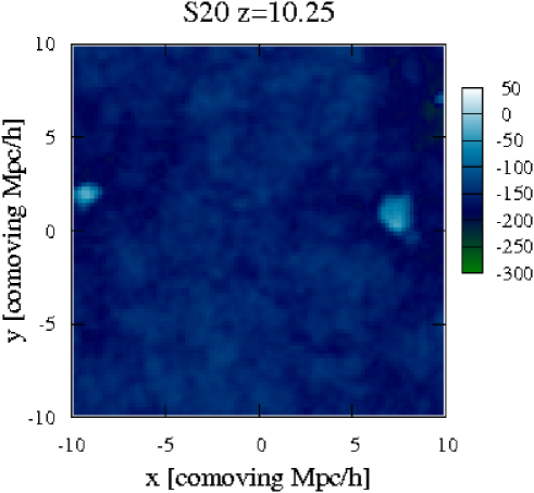
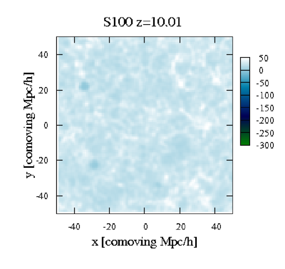
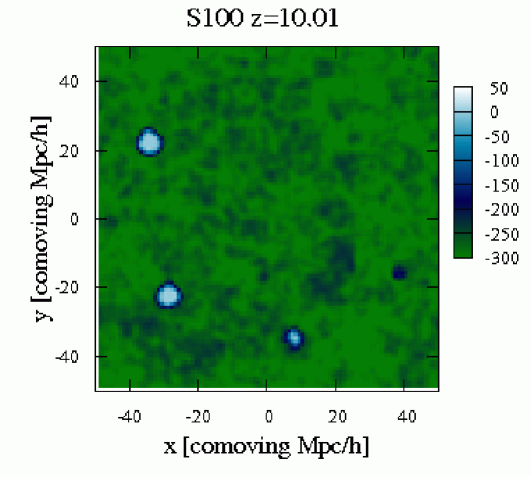
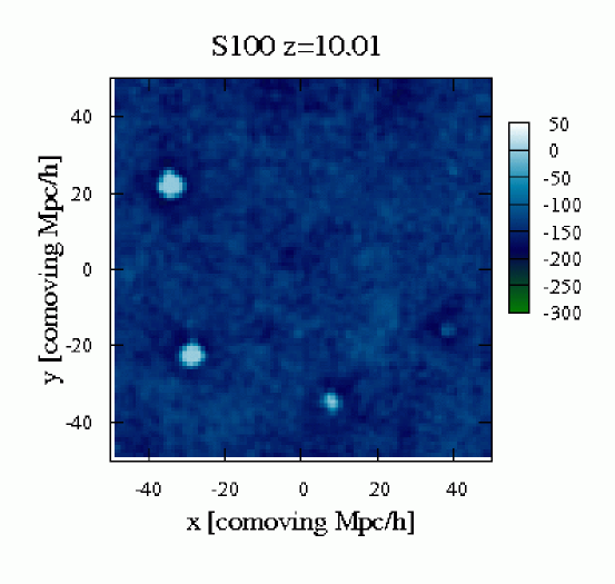
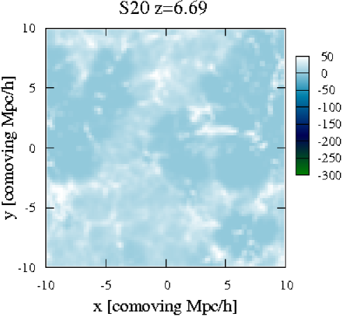
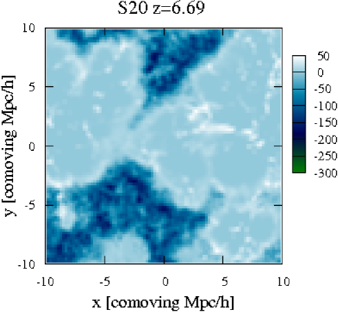
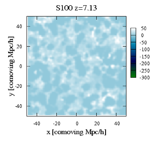
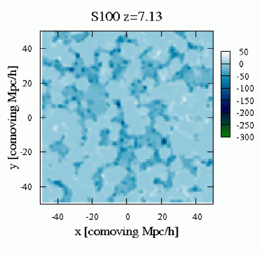
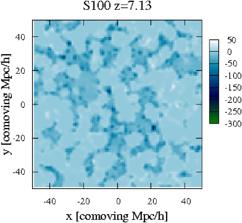
Figure 12: Differential brightness temperature maps for both box sizes and 3 different hypotheses for computing the spin temperature (see main text and description in the figure). The redshift of the 6 top panels is chosen such that $\langle x_{\alpha}\rangle=1$, the redshift of the 6 bottom panels is such that $\langle x_{H}\rangle=0.5$. The temperature color scale is linear, in mK. The thickness of the slice is $2\,h^{-1}\,\rm{Mpc}$ .

The six bottom panels of Fig. 12 shows the same maps for the HRR. At this redshift we have $\langle x_{\alpha}\rangle>200$ for both simulations. Consequently the maps for cases 2 and 3 are almost identical. Comparing with Fig. 10 it can be checked that the regions which are still seen in absorption are the neutral regions not too close to the ionization fronts. Comparing the absorption regions in the S20 and in the S100 maps, it can be seen that the signal is somewhat stronger in the S20 simulation. We have determined that a lower gas kinetic temperature in the S20 simulation, in the voids, is responsible for this effect. Since we are talking about temperatures lower than $10$ K, a difference of a few K produce a large effect on the differential brightness temperature. The S20 simulation has a higher mass resolution which creates higher density contrasts. In the voids, the density is lower and the adiabatic expansion stronger : the resulting temperature is lower.

Obviously, in case 1, the absorption regions turn to emission. Since emission saturates quickly at a few tens of mK, the statistical property of the signal such as the average rms fluctuations of the brightness temperature will be weaker. At such an advanced stage in the reionization history the assumption made in case 1 may actually be more realistic: case 2 and 3 would probably look more like case 1 if we included X-ray sources.

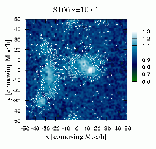
Figure 13: Ratio of the differential brightness temperature computed with the fluctuating local value of $x_{\alpha}$ on the one hand and the average value of $x_{\alpha}$ on the other hand. The color scale is linear. The contour is computed from the $x_{\alpha}$ field for the $x_{\alpha}=1$ value.

Using a homogeneous average value for $x_{\alpha}$ to account for the Wouthuysen-field effect ( for example a calibrated function of $x_{H}$) is much easier than computing the full radiative transfer in the line. So it is important to assess the benefit reaped from doing the full treatment. The $x_{\alpha}$ field induces its own fluctuation in the brightness temperature signal. Fig. 13 illustrates this point. It shows a map of the ratio of the differential brightness temperatures computed with the fluctuating local value of $x_{\alpha}$ on the one hand and the homogeneous, average value of $x_{\alpha}$ on the other hand. This map is computed at the WFCR, for the S100 simulation. As expected, the ratio is mostly larger than one inside the $x_{\alpha}=1$ contour and lower outside. Moreover the two differential brightness temperatures differ by up to 30%. Consequently it appears that, at these early redshifts when the Lyman-$\alpha$ coupling is not full, it is worth doing the full Lyman-$\alpha$ transfer.

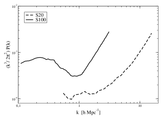
Figure 14: 3D isotropic power spectrum of ${x_{\alpha}\over 1+x_{\alpha}}$. The spectra are plotted for both simulations, S20 and S100, at the redshift when $\langle x_{\alpha}\rangle=1$.

Using the power spectrum as a statistical tool for analyzing the EoR $21\,\rm{cm}$ signal is natural because it can be directly computed from the visibilities measured by the radio interferometers such as LOFAR, MWA or SKA. Morales & Hewitt (Morales04 (2004)) have shown that using the full 3D power spectrum rather than the 2D angular power spectrum will improve the sensitivity of the observations and make the process of foreground removal easier.

4.2.4 Strength of the Lyman-$\alpha$ coupling fluctuations

Fig. 14 shows the power spectrum of the quantity $z_{\alpha}={x_{\alpha}\over 1+x_{\alpha}}$ for both simulations at the WFCR. Indeed directly plotting the spectrum of $x_{\alpha}$ is not interesting : the $x_{\alpha}$ field is dominated by the very strong values near the sources and has a power spectrum similar to that of a distribution of Dirac functions. However, these very high values of $x_{\alpha}$ are not especially interesting : they are just values for which the coupling saturates. $z_{\alpha}$, which is just the weight applied to the inverse kinetic temperature in Eq. $9$ (neglecting the contribution of $x_{c}$), varies between $0$ and $1$ and contains more relevant information about the magnitude of the coupling. As can be seen in Fig. 14, the point sources still dominate the small scales. More interesting is the increase of the power spectrum toward large scales, which is barely visible for the S20 simulation but obvious in the S100 simulation. It is likely that this increase tracks the Poisson noise in the large scale clustering of the sources and void distribution. For the S100 simulation, the spectrum shows a local maximum at scales $\sim 30\,h^{-1}\,\rm{Mpc}$. Whether this maximum is real or only the effect of the box size is an interesting question. Only simulations with larger boxes will give the answer.

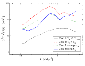
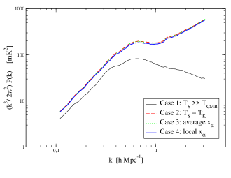
Figure 15: Comparison of the 3D isotropic dimensional power spectrum of the differential brightness temperature with 4 different assumptions used to compute the spin temperature (see legend and main text). The spectra are computed for the S100 simulation. The top panel is for the redshift when $\langle x_{\alpha}\rangle=1.$ and the bottom panel is for the redshift when $\langle x_{H}\rangle=0.5$.

4.2.5 Differential brightness temperature

In this section, we will compute directly the dimensional power spectrum of $\delta T_{b}$. Various authors, studying the emission regime, compute the power spectrum of $\delta T_{b}$ divided by the average, redshift dependent, emission temperature $T_{0}\sim 28\left({1+z\over 10}\right)^{1/2}$. When we include the absorption regime, $T_{0}$ has no special significance. Using the actual average $\delta T_{b}$ of the box would be no better : having both emission and absorption, it holds no information about the amplitude of the fluctuations and may even be zero at some redshift. Using the actual rms average at each redshift would indeed be more relevant as it does reflect the amplitude of the fluctuations. However it would erase the information about the absolute amplitude at a given scale, at different redshifts. Consequently, we decided to plot the direct dimensional power spectrum of the differential brightness temperature.

         

Figure 16: 3D isotropic dimensional power spectrum of the differential brightness temperature for the two box sizes. The stage of reionization is indicated in each panel. The four left panels assume $T_{S}\gg T_{CMB}$ while the four right panels compute $T_{S}$ exactly using the local values of $x_{\alpha}$.

Fig. 15 shows the three-dimensional isotropic power spectrum of $\delta T_{b}$ as defined by Eq. $8$ for the S100 simulation, at the WFCR (top panel) and the HRR (bottom panel), in four different cases for the computation of the spin temperature. In case 1, we assume that $T_{S}\gg T_{CMB}$, in case 2 $T_{S}=T_{K}$, in case 3 we use Eq. $9$ with the box averaged value of $x_{\alpha}$, and finally in case 4, we use Eq. $9$ with the local values of $x_{\alpha}$. As expected, the larger differences appear at the WFCR, where the amplitude of the power spectrum changes by more than a factor of 10 depending on the case. Case 1, ignoring the possibility of absorption, strongly underestimates the amplitude of the power spectrum, while case 2, assuming full coupling between spin temperature and gas kinetic temperature, overestimates the amplitude. The amplitudes for cases 3 and 4 are similar (and more realistic). However, case 4 shows more power at small scales and less power at large scales than case 3. Indeed, as illustrated in Fig. 13, case 3 uses a larger value of $x_{\alpha}$ far from the sources, thus produces a stronger absorption in large scale voids and more power at large scale in the spectrum than case 4. The behaviour at small scales arises from the presence of the Ly-$\alpha$ halos around the sources in case 4. Semelin et al. (Semelin07 (2007)) have shown that the profile of these halos can be as steep as $r^{-3}$ if the gas has an isothermal profile. Even at distances of a few comoving Mpc, where the gas profile flattens, the Ly-$\alpha$ halo profile behaves as $\sim r^{-2.3}$ (Semelin et al. Semelin07 (2007), Chuzhoy & Zheng Chuzhoy07 (2007)). The contribution from these sharp $x_{\alpha}$ fluctuations explains the increase in the case 4 power spectrum at small scales. At the HRR (bottom panel) the situation is simpler. The Wouthuysen-Field coupling is very strong and case 2, 3 and 4 are almost indistinguishable. All three have much larger amplitude than case 1 which is related to the fact that absorption can produce a larger absolute signal than emission, thus larger fluctuations. It is interesting to notice that the difference in amplitude is especially large at small scales. The contribution of the regions straddling the sharp ionization front is presumably responsible for this feature. In case 1, the brightness temperature rises from $\sim 0\,\rm{mK}$ in the fully ionized region inside the ionization front to a moderate $\sim 20\,\rm{mK}$ emission outside of the front. In all other cases, the temperature first rises to a moderate emission in the regions just outside the ionization front, preheated above the CMB temperature by the hard part of the source spectrum, then drops to strong absorption farther out in the cool voids. The thickness of the preheated regions depends strongly on the source modeling : in our case it is less than $1\,h^{-1}\,\rm{Mpc}$ . With a harder spectrum these regions would be thicker, and with X-ray sources they would be erased and the corresponding feature absent in the power spectrum.

Fig. 16 shows the $\delta T_{b}$ power spectrum of both the S20 and S100 simulations at four different stages of reionization (the WFCR, $\langle x_{H}\rangle=0.1$, $\langle x_{H}\rangle=0.5$, and $\langle x_{H}\rangle=0.9$), for case 1 (the four panels on the left) and case 4 (the four panels on the right). Let us first comment on how the spectra for the two simulations connect. In most cases the large scales in the S20 simulation have less power than the same scales in the S100 simulation. This is the reason why EoR simulations have to use large boxes : to sample well enough the large scale clustering properties of the source distribution. There is however one exception, the $\langle x_{H}\rangle=0.5$ (HRR) in case 4, where the S20 simulation has more power even on its large scales. This is related to the fact, already discussed in section 4.2.3, that the absorption in the voids is stronger in the S20 simulation and thus the fluctuations are amplified. A second point is that at the WFCR the case 4 spectra have a more complex signature and a larger amplitude than the case 1 spectra which merely track the density fluctuations. Taking absorption and Ly-$\alpha$ coupling correctly into account is essential at this early redshift. A third point is that we reproduce the behaviour noted by Mellema et al. (2006b ) and Lidz et al. (2007b ), that at scales of a few comoving Mpc the amplitude of the power spectrum reaches a maximum at the HRR, then decreases. This is true for case 1, which was used by Lidz et al. In case 4, with the full Ly-$\alpha$ modeling, it looks like the maximum shifts to smaller values of the average ionization fraction.

5 Conclusions

In this work, we have presented simulations of the $21\,\rm{cm}$ emission from the EoR. The first hydrodynamic simulations were run in cosmological boxes of sizes $20\,h^{-1}\,\rm{Mpc}$ and $100\,h^{-1}\,\rm{Mpc}$ with $2\times 256^{3}$ particles. Then, using our adaptive Monte-Carlo code LICORICE, we ran, in post-treatment, radiative transfer simulations for the ionizing continuum. Finally cosmological radiative transfer simulations in the Lyman-$\alpha$ line were performed. The latter are necessary to compute the neutral hydrogen spin temperature without making any assumption about the strength of the coupling. This approach has not been followed before. We model the sources of both ionizing continuum and Lyman-$\alpha$ photons as stars, using a Salpeter IMF cut off at $100$ M_⊙. The $100\,h^{-1}\,\rm{Mpc}$ simulation star formation history is calibrated on the $20\,h^{-1}\,\rm{Mpc}$. The photon escape fraction is calibrated independently in both simulations to produce a Thomson scattering optical depth of CMB photons within $1\sigma$ of the WMAP3 value, and a complete reionization at redshift $z\sim 6$. We have not included X-ray sources. If we had they would heat up the IGM and reduce the contribution of absorption vs emission in the signal.

We first computed the evolution of a number of box-averaged quantities as functions of the average ionization fraction. We find that, with our source modeling, the average Lyman-$\alpha$ coupling coefficient $x_{\alpha}$ reaches 1 for small values of the ionization fraction (a few $10^{-3}$). However full coupling ($x_{\alpha}\gg 1$) is achieved only for ionization fractions greater than $10^{-1}$. This is in line with expectations. Next we plotted the average spin temperature and differential brightness temperature. It was shown that the results are very different depending on how the average is computed : directly on the spin$\backslash$brightness temperature of the particles, or from the volume-averaged values of the gas kinetic temperature and coupling coefficients. The latter is often used, but the former is more relevant. The direct average tends to erase the signal as regions in absorption have a much stronger signal than regions in emission. Maps of the $21\,\rm{cm}$ emission confirm that the different assumptions made in computing the spin temperature lead to very different levels of the signal. The $T_{S}\gg T_{CMB}$ assumption is not relevant at all for our choice of source modeling. It would be more relevant at not-too-early redshifts if we included X-ray sources. As expected the full coupling assumption, $x_{\alpha}=\infty$, is reasonable except in the early phase of reionization. In this early phase, we illustrate how computing the local values of $x_{\alpha}$ produces large fluctuations in the brightness temperature compared to using a redshift-dependent uniform value.

Finally the 3D dimensional power spectrum of the differential brightness temperature was plotted, with different assumptions in computing the spin temperature, at various stages of reionization and for the two box sizes. The first important (and expected) result is that including the possibility of a signal seen in absorption adds a large amount of amplitude to the power spectrum. This obviously depends on the choice of the source model. Then, in the early phase of reionization ($\langle x_{H}\rangle<0.1$), using the local value of the Lyman-$\alpha$ coupling changes the spectrum by transferring power from large scales to small scales. We reproduce the behaviour shown by Mellema et al. (2006b ) and Lidz et al. (2007b ) : a maximum of the amplitude at $\langle x_{H}\rangle=0.5$ for the scales around $10\,h^{-1}\,\rm{Mpc}$. However, when absorption and the exact computation of the Lyman-$\alpha$ coupling are included, this maximum is shifted to smaller ionization fractions.

As mentioned several times, the first modification to our model that will be investigated is a modification of the source model. Including even a limited number of X-ray sources such as quasars would more efficiently preheat the regions outside of the ionization front, reducing the strength of the absorption regime, or even turning it to emission. This will be investigated in a forthcoming paper.

Another interesting development of this work is to include the anisotropic effect of the peculiar velocities on the $21\,\rm{cm}$ emission (Barkana & Loeb 2005a ). Using the anisotropy, it is possible to separate the contribution of the velocities to the $21\,\rm{cm}$ fluctuations from the other contributions and to derive constraints on the cosmological parameters. Since this effect is important mostly in the early reionization phase and on small scales, it is a logical follow-up of including the full modeling of the Lyman-$\alpha$ coupling.

The implication of this work for the design of the future radio interferometers is simply to emphasize the potential for the detection of the signal during the early phase of reionization when the fluctuations in the signal are strong. Unfortunately, translating ”early phase” into a numerical value for the redshift depends crucially on the star formation history at these high redshifts, of which very little is known. From the value of the Thomson scattering optical depth, it is likely, however, that this early phase occurs at $z>12$.

- (1) Ahn, S.-H., Lee, H.-W., & Lee H. M., 2001, ApJ, 554, 604
- (2) Ahn, S.-H., Lee, H.-W., & Lee, H. M., 2002, ApJ, 567, 922
- (3) Aller, L. H. Numerical Data and Functional Relationships in Science and Technology - New Series ” Gruppe/Group 6 Astronomy and Astrophysics ” Volume 2 , Springer-Verlag Berlin Heidelberg New York
- (4) Altay G., Croft, R. A. C., & Pelupssy, I., 2008, MNRAS, 386, 1931
- (5) Avery, L. W., & House, L. L., 1968, ApJ, 152, 493
- (6) Barkana, R., & Loeb, A., 2004, ApJ ,609, 474
- (7) Barkana, R., & Loeb, A., 2005a, ApJ, 624, L65
- (8) Barkana, R., & Loeb, A., 2005b, ApJ, 626, 1
- (9) Bertschinger, E., 2001, ApJS, 137, 1
- (10) Cantalupo, S., Porciani, C., Lilly, S., & Miniati, F., 2005, ApJ, 628, 61
- (11) Cen, R., 1992, ApJS, 78, 341
- (12) Chuzhoy, L. & Shapiro P.R., 2006, ApJ, 651, 1
- (13) Chuzhoy, L. & Zheng, Z.., 2007, ApJ 670, 912
- (14) Ciardi, B., Madau., P., 2003, ApJ, 596, 1
- (15) Ciardi, B., Scannapieco, E., Stoehr, F. et al., 2006, MNRAS, 366, 689
- (16) Crocce, M., Pueblas, S., & Scoccimarro, 2006, MNRAS, 373, 369
- (17) Dijkstra, M., Haiman, Z., & Spaans, M., 2006, ApJ, 649, 14
- (18) Fan, X., Carilli, C. L., & Keating, B., 2006, ARA&A, 44, 415
- (19) Faucher-Giguère, C.-A., Lidz, A., Hernquist, L., & Zaldarriaga, M., 2008, ApJ, 682, L9
- (20) Field, G. B., 1958, Proc. IRE, 46, 240
- (21) Furlanetto, S. R., Sokasian, A., & Hernquist, L., 2004, MNRAS, 347, 187
- (22) Furlanetto, S. R., Oh, S. P., & Briggs, F. H., 2006a, PhR, 433, 181
- (23) Furlanetto, S. R. & Pritchard, J. R., 2006b, MNRAS, 372, 1093
- (24) Furlanetto, S. R. & Peng Oh, S., 2006c, ApJ, 652, 849
- (25) Glover, S. C. O. & Brand, P. W. J. L., 2003, MNRAS, 340, 210
- (26) Gnedin, N. Y. & Ostriker J. P., 1997, ApJ, 486, 581
- (27) Gnedin, N. Y. & Abel, T., 2001, NewA, 6, 437
- (28) Gnedin, N. Y. & Shaver, P. A., 2004, ApJ, 608, 611
- (29) Haardt, F. & Madau, P., 1996, ApJ, 461, 20
- (30) Gunn, J. E. & Peterson, B. A., 1965, ApJ, 142, 1633
- (31) Hernquist L. & Katz N. 1989, ApJS, 70, 419
- (32) Iliev, I. T., Shapiro, P. R., Ferrara, A., & Martel, H., 2002, ApJ, 573, L123
- (33) Iliev, I. T., Mellema, G., Pen, U.-L.,et al., 2006, MNRAS, 369, 1625
- (34) Iliev, I. T., Mallema, G., Shapiro, P. R., & Pen, U., 2007, MNRAS, 376, 534
- (35) Iliev, I. T., Mellema, G., Pen, U-L., Bond, J. R., & Shapiro, P. R., 2008, MNRAS, 384, 863
- (36) Katz, N., Weinberg, D. H., & Hernquist, L., 1996, ApJS, 105, 19
- (37) Komatsu, E., Dunkley, J., Nolta, M. R., et al., 2008, arXiv:0803.0547
- (38) Kuhlen, M., Madau, P., & Montgomery, R., 2006, ApJ, 637, L1
- (39) Lidz, A., Zahn, O., McQuinn, M., et al., 2007a, ApJ, 659, 865
- (40) Lidz, A., Zahn, O., McQuinn, M., Zaldarriaga, M., & Hernquist, L., 2007b, arXiv:0711.4373
- (41) Liszt, H., 2001, A&A, 371, 698
- (42) Loeb, A. & Rybicki, G., 1999, ApJ, 524, 527
- (43) Madau P., Meiksin A., Rees M. J., 1997, ApJ, 475, 429
- (44) Maselli, A., Ferrara, A., & Ciardi, B., 2003, MNRAS, 345, 379
- (45) McQuinn, M., Zahn, O., Zaldarriaga, M., Hernquist, L., & Furlanetto, S., 2006, ApJ, 653, 815
- (46) McQuinn, M., Lidz, A., Zahn, O., et al., 2007, MNRAS, 377, 1043
- (47) Mellema, G., Iliev, I. T., Alvarez, M. A., & Shapiro, P. R., 2006a, NewA, 11, 374
- (48) Mellema, G., Iliev, I. T., Pen, U.-L., & Shapiro, P. R., 2006b, MNRAS, 372, 679
- (49) Metcalf, R. B., & White, S. D. M., 2007, MNRAS, 381, 447
- (50) Mesinger, A. & Furlanetto, S., 2007, ApJ, 669, 663
- (51) Monaghan, J. J., 1992, Ann. Rev. A&A, 30, 543
- (52) Morales, M. & Hewitt, J., 2004, ApJ, 615, 7
- (53) Nakamoto, T., Umemura, M., & Susa, H., 2001, MNRAS, 321, 593
- (54) Naoz, S. & Barkana, R., 2008, MNRAS, 385, L63
- (55) Pawlik, A. H. & Schaye, J., 2008, MNRAS, 389, 651
- (56) Pritchard, J. & Furlanetto, S. R., 2007, MNRAS, 376, 1680
- (57) Rasera, Y. & Teyssier, R., 2006, A&A, 445, 1
- (58) Razoumov, A. O., & Cardall, C. Y., 2005, MNRAS, 362, 1413
- (59) Rijkhorst, E.-J., Plewa, T., Dubey, A., & Mellema, G., 2006, A&A, 452, 907
- (60) Salvaterra, R., Ciardi, B., Ferrara, A., & Baccigalupi, C., 2005, MNRAS, 360, 1063
- (61) Santos, M. G., Amblard, A., Pritchard, J., et al., 2007, arXiv:0708.2424
- (62) Seager, S., Sasselov, D. & Scott, D., 1999, ApJ, 523, L1
- (63) Semelin, B., Combes, F., & Baek, S., 2007, A&A, 474, 365
- (64) Shapiro, P. R. & Giroux, M. L., 1987, ApJ, 321, L107
- (65) Shapiro, P. R., Ahn, K., Alvarez, M. A., et al., 2006, ApJ, 646, 681
- (66) Spergel, D. N., Bean, R., Doré, O., et al., 2007, ApJS, 170, 377
- (67) Spitzer, L. 1978, Physical Processes in the Interstellar Medium (New York: Wiley)
- (68) Springel, V., & Hernquist, L., 2003, MNRAS, 339, 289
- (69) Springel, V., 2005, MNRAS, 364, 1105
- (70) Susa, H., 2006, PASJ, 58, 445
- (71) Tasitsiomi, A., 2006, ApJ, 645, 792
- (72) Theuns, T., Leonard, A., Efstathiou, G., Pearce, F. R., & Thomas, P. A., 1998, MNRAS, 1998, 301, 478
- (73) Trac, H., Cen, R., 2007, ApJ, 671, 1
- (74) Valdés, M., Ciardi, B., Ferrara, A., Johnston-Hollitt, M., & R’́ottgering, H., 2006, MNRAS, 369, L66
- (75) Verhamme, A., Schaerer, D., & Maselli, A., 2006, A&A, 460, 397
- (76) Whalen, D., & Norman, M. L., 2006, ApJS, 162, 281
- (77) Wouthuysen S. A., 1952, AJ, 57, 31
- (78) Zahn, O., Lidz, A., McQuinn, M., et al. 2007, ApJ, 654, 12
- (79) Zheng, Z. & Miralda-Escudé, J., 2002, ApJ, 578, 33