Abstract
The equilibration of matter and onset of hydrodynamics can be understood in the AdS/CFT context as a gravitational collapse process, in which “collision debris” create a horizon. In this paper we consider the simplest geometry possible, a flat shell (or membrane) falling in the holographic direction toward the horizon. The metric is a combination of two well known solutions: thermal AdS above the shell and pure AdS below, while motion of the shell is given by the Israel junction condition. Furthermore, when the shell motion can be considered slow, we were able to solve for two-point functions of all boundary stress tensor and found that an observer on the boundary sees a very peculiar : while the average stress tensor contains the equilibrium plasma energy and pressure at all times, the spectral densities of the correlators (related with occupation probabilities of the modes) reveal additional oscillating terms absent in equilibrium. This is explained by the “echo” phenomenon, a partial return of the field coherence at certain “echo” times.
Toward the AdS/CFT Gravity Dual for High Energy Collisions. 3.Gravitationally Collapsing Shell and Quasiequilibrium
Shu Lin111E-mail:slin@grad.physics.sunysb.edu, and Edward Shuryak222E-mail:shuryak@tonic.physics.sunysb.edu
Department of Physics and Astronomy, SUNY Stony-Brook, NY 11794
1 Introduction
Observation at RHIC of collective flows in relativistic heavy ion collisions, well described by ideal hydrodynamics [2, 3] have lead to a paradigm shift in the field toward studies of strongly coupled plasmas. AdS/CFT correspondence [1] is one of actively pursuit directions, both for understanding of strongly coupled gauge theories in general and properties of Quark-Gluon Plasma (QGP) in particularly: for recent review see [4].
This paper continues the line of work of our two previous papers, [5] and [6], which we will call I and II respectively below. Those papers include extensive introduction explaining our approach to the problem, which we will not repeat here. Let us just say that in those works we dealt with “elementary” collisions – calculating the shape of the falling string between two departing charges and its hologram at the boundary – which in the QCD language can be related to annihilation into a pair of heavy quarks or collisions. Thus in I and II there was no horizon on the gravity side and no temperature or entropy on the matter side. In this paper we address these issues, related with heavy ion collisions and equilibration.
Properties of equilibrium strongly coupled conformal plasma is by now well studied in significant detail in the AdS setting, in static thermal AdS-BH metric suggested by Witten. Many details about quasinormal modes of this metric and in particularly the correlators of stress tensors and their spectral densities are known, we especially recommend [8, 9, 11, 10]. Recent developments included flowing near-equilibrium state, with slowly/gradually deformed horizons and derivation of hydrodynamics up to second order in gradients: we will not use those here, see references in a review [4].
The most challenging task of the theory now is the understanding of how matter manages to equilibrate so rapidly in RHIC collisions, and what exactly such equilibration means microscopically. The success of hydrodynamics in describing RHIC elliptic flow data seems to suggest the thermalization time of the order of , yet its mechanism remains unclear. The quest for its mechanism involves studies of various phenomenology and theoretical approaches. We will not attempt to review it and just mention one approach to ideas of which we will refer below, the “Glasma model”: see Ref.[7] and references therein. It is based on classical Yang-Mills equations and starts with the so called Color Glass Condensate initial condition. While the coupling is assumed weak in this approach, strong coherent fields make its behavior nonperturbative.
Our approach also attempts to address the transition from Glasma-like initial coherent gauge fields to incoherent near-thermal QGP, but in strong coupling and thus the AdS/CFT setting. Since the vacuum corresponds to extremal black hole solution – pure AdS geometry without a horizon – while the thermal field theory is dual to AdS black hole with a horizon, the main issue is how deposition of an extra mass – from “debris” of the collision – leads to excitation of the extremal to non-extremal black hole and dynamical creation of the horizon. In simpler words, we have to follow some kind of a gravitational collapse.
In I and II we already discuss qualitatively how falling debris created in the collisions – e.g. large number of falling strings between departing charges – make a falling matter shell or membrane. While in I we studied its fall ignoring its own weight, we have to include it now, as its near-horizon breaking is entirely due to adding the mass of the shell to total gravity. We have argued in those papers that in principle one can address the problem by following the motion of two membranes, the and that describing (a la “membrane paradigm” see book by Thorne and collaborators [16]).
For now we do not study motion of those two membranes in realistic geometry, for obvious reasons starting with the simplest geometry possible. We assume that the matter shell (and thus the horizon) is – that is independent on our world 3 spatial coordinates, and moves only in the 5-th holographic direction#1#1#1the equilibration in this setting is not due to spatial gradient as in hydrodynamics. The setup of this gravitational collapse model is described in Sec.2. The equation of motion for the shell is given by Israel junction condition[17] which we solve numerically. We find how its trajectory depends on the property of the shell; but in all cases the distant observer sees its slow approach to the horizon at late time.
Early works along this path include important papers [12, 13, 14] which we partly follow. They consider a collapsing shell geometry, but unlike us they use as a probe some bulk scalar field and we don’t find their boundary conditions at the shell sufficiently convincing, and we tried to improve those by using gravitons instead.
What the observer sees as the shell falls is dual to the evolution of SYM from certain initial ensemble to the final thermal equilibrium. The insight into the problem of thermalization is thus obtained by studying various observables – the induced stress tensor and its correlation functions on the boundary – while the shell is somewhere in its process of falling. The former is given by one-point function and the metric above the shell, which in our geometry is time AdS black hole metric. Thus the “single point observer” who is only able to measure the average density and pressure would be driven to the conclusion that the matter is fully equilibrated at all times. More sophisticated “two point observer”– measuring the stress tensor correlation functions – would however be able to see the deviations the from the thermal ensemble. We compute those deviations in Sec. 3, using various components of the graviton perturbations to probe the gravitational background with a shell.
As a significant technical advance of this work, we show that unique prescription for boundary conditions for the gravity waves on the shell follows from the junction condition itself. Thus we show how correctly propagate the graviton wave across the shell, relating the obvious infalling conditions near the AdS center to what is seen on the boundary. Explicit expressions are obtained for two-point function in near equilibrium stages, when the shell is close to the horizon. We solve the wave equations both numerically and using the WKB approximation, finding good agreement between the two. Possible implications of the results are finally summarized and discussed in Sec.4.
2 Gravitationally collapsing shell in AdS
2.1 The background metric
Our setting includes the basic AdS background, described by the metric . Its holographic coordinate is zero at the boundary (UV) and infinity at the AdS center (IR). The problem considered is a simple generalization of Israel’s original problem, which was collapsing spherical shell in asymptotically flat 3d space. And it shares its main feature: although the shell is falling with its radial position time depending, the gravity both inside and outside it is time independent. Furthermore, inside a sphere there is no influence of the shell’s existence at all: the famous statement going back to Newton himself. The gravity outside only knows the total shell mass.
It is not difficult to prove that the same is true for flat shell in the AdS setting as well. Starting with a generic form:
| (1) |
one can set by a coordinate transformation. The metric has to satisfy the vacuum Einstein equation
| (2) |
with both above#2#2#2The reader is reminded that the coordinate is inversely proportional to radial coordinate, thus somewhat counterintuitive inequalities. and below the shell’s position . We will also refer to those as “outside” and “inside” regions below.
The component tells us that . The , equations are used to obtain:
| (3) |
can be dropped by a rescaling in the coordinate. Now we require the metric should reduce to the AdS form infinitely far away from the shell. as , we can have , then outside the shell the metric is in form of translationally invariant AdS-black hole(AdS-BH). On the other hand, inside at the AdS center we have to set to suppress the term. Therefore the inside is just AdS metric.
So the background metric is the combination of AdS-BH and AdS, with the two metrics separated by a shell. We will use the metric in the usual form
| (4) |
with (or ) outside (or inside) the shell position . and are both continuous in order for to match.
Note that a singularity at is outside the region where the former metric is used, as . This does not mean that there is no horizon in the problem: in spite of pure AdS metric inside, the dynamical horizon and trapped surface (both time dependent) do exists.
2.2 Israel junction conditions and the falling shell
As in [5], the strings in AdS bulk were modeled by a shell (membrane), the action of which is given by:
| (5) |
where is the induced metric on the shell. is the only parameter characterizing the shell.
We use Lanczos equation to study the falling of the shell:
| (6) |
where and
We parametrize the induced metric on the shell as follows:
| (7) |
We choose and Assume the EOM is given by .
The norm is determined from the condition and as:
| (8) |
Note here the norm points to the AdS center(). Therefore we have :inside; :outside
The curvature K is calculated as follows:
| (9) | |||
| (10) |
is determined from the shell action: . (6) becomes:
| (11) | |||
| (12) |
| (13) | |||
| (14) |
| (15) |
The falling velocity seen by distant observer is given by:
| (16) |
Suppose the shell starts falling at with vanishing initial velocity. The horizon radius can be expressed in terms of and :
| (17) |
Note (17) implies another constraint . The independent parameters and should be estimated from the initial conditions(e.g. energy density, particle number), these will determine the equilibrium temperature of the evolution.
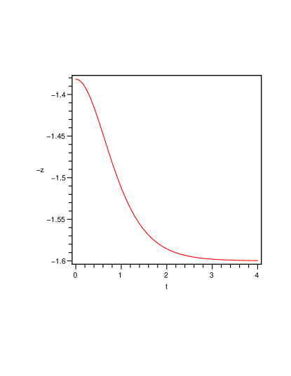
With chosen parameters, it is easy to integrate (16) to give the trajectory of the shell. We have plotted the shell trajectory in Fig.1. It shows three stages of falling, initial acceleration (), intermediate near-constant velocity fall, and the final near-horizon freezing with exponentially small deviation ().
Finally, what are the physical meaning of the parameters of our model, the initial position and the shell tension ? The wave functions of the colliding nuclei are believed to be [18] concentrated at the certain momentum scale called the “saturation scale” , which depends on collision energy and nuclei: it is about 1.5 GeV at RHIC. The holographic coordinate has the meaning of the inverse momentum scale in the renormalization group sense, thus its initial value should be identified with inverses saturation scale . Further “falling” corresponds to motion of the wave function into the infrared direction, till equilibrium is reached. The initial temperatures at RHIC (and thus are believed to be about .35 , with : thus the expected inequality is satisfied.
(Physical fireballs not only equilibrate but also expand, with decreasing by a factor 3-4 in RHIC collisions. This would correspond to a horizon toward larger , as suggested in [19], but this feature is of course not included in the present model.)
The corresponding tension of the shell may be calculated from (17). Although we do not follow this direction here, one may attempt to calculate it in a particular model of the collisions. In particular, the so called Lund model prescribe how many color strings per transverse area is created, and as the shell is but an approximation to all those strings falling together, its tension may be identified with the of the tensions of all the strings.
3 Correlation functions of the Gauge Theory
With the complete gravity background at hand, we are ready to study the property of the dual gauge theory under thermalization. We already commented that since the metric is asymptoticly AdS-BH, the one-point function of the stress tensor is the same as thermal SYM result. Therefore we consider the two-point functions as the expected place to find deviations from the equilibrated thermal ensemble.
The most standard way is to study a probe field in the background which is dual to some boundary operator, then use AdS/CFT prescription to find the correlation function. The simplest probe field used in early works was the bulk scalar [12, 13, 14]. However we choose to use various components of the metric field, , which is dual to the boundary stress tensor. One obvious reason is to avoid the introduction of new field into the problem. The other reason involves the matching condition of on the shell, as will become clear later. Also we only probe the geometry after the creation of the shell.
Thus we solve for the metric perturbation propagating in the bulk specified above. This is a very difficult task in general, because the shell is always falling and thus there are time dependent boundary condition at the shell: this makes a straightforward Fourier decomposition in time impossible. However, a possible simplification can be made if the Fourier mode is much faster than the falling of shell, i.e. the condition holds, we may consider the shell as quasi-static. In this limit, we can trust the Fourier mode and study the problem in the usual way. In other words, we only trust quantities obtained for . With this argument, we can in principle study two-point function in any stage provided the mode is fast enough.
3.1 Matching Condition on the Shell
Israel junction condition in general should be applicable for any gravity fields. Therefore, one can apply it for background plus graviton perturbation and from the latter obtain the matching condition for the graviton.
Similar as in Sec.2.2, we start with the Lanczos equation:
| (18) |
which we cast into a different form:
| (19) |
The zeroth order (in ) Lanczos equation have already been used above, for calculation of the trajectory of the shell. Now we require vanishing of the first order terms in Lanczos equation
| (20) |
with and . remains unchanged, so the variation of comes entirely from Christoffel:
| (21) |
We choose the gauge and further assume , where ,,. This will not affect the two-point function because the gravity background is rotationally invariant in Calculating the variation of Christoffel to the first order in and noting , (quasi-static limit), we find the only non-vanishing components of is:
We have omitted some components involving index : those can be obtained by the substitution from those listed above. Plugging to (19), we have:
| (22) |
We use from here on and for metric perturbations inside and outside the shell respectively. All the quantities are evaluated on the shell . The other identities follow from the continuity of induced metric across the shell.
Note the jump in time coordinate, we have to do the Fourier transform in a consistent way#3#3#3The convention we use is : , The indices “in” and “out” represent quantities inside and outside the shell. We use as the frequency measured by clock outside the shell, the corresponding frequency inside is given by . Thus we obtain from (3.1):
| (23) |
All the quantities are evaluated on the shell
From here on, we define in accordance with the literature[20]. The axial gauge is just . The metric perturbations can be classified into three channels, according to [9]: scalar channel: shear channel: and sound channel include , , and
The metric perturbations satisfy linearized Einstein equation, and they are determined up to residual gauge transformation where should preserve the axial gauge chosen above. Instead of fixing the gauge, one can look for gauge invariant combination in each channel. The behavior of these gauge invariant objects encodes complete information of retarded correlator[9, 21].#4#4#4there is a subtlety in the sound channel, which will be elaborated later
3.1.1 The scalar channel
The gauge invariant object is simply outside the shell and inside. The EOM of is given by(with corresponding to )
| (24) |
The prime denote derivative with respect to . The matching condition between and can be easily obtained from (3.1):
| (25) |
Besides the matching condition (3.1.1), we also need boundary condition at AdS center to uniquely fix the solution of in the bulk up to normalization. The boundary condition we use at AdS center is infalling wave or regular wave. With these conditions, we are ready to proceed. Let us start from inside the shell: is given by the solution to the following equation:
| (26) |
where . It origins from the jump of frequency across the shell. The EOM can be solved in terms of cylindrical function:
| (30) |
While outside the shell, can be written as a linear combination of two independent solutions, which we select to be the infalling wave and the outfalling waves at the horizon#5#5#5Note that it is just a formal basis for the solution above, we don’t use it below the shell and there is no horizon singularity there.
| (31) |
| (32) |
where , .
We expect to recover the equilibration because, as the shell approaches the “horizon”, the region where geometry deviates from AdS-BH shrinks exponentially. The ratio . All deviations from equilibrium should become exponentially small as well, as we expect from any other small deviations from equilibrium.
We would like to confirm this limit by our matching/boundary condition. As the shell approaches the “horizon”, ,, we may disregard the third situation in (30). We want to calculate the ratio to the leading order in or . The correction to is linear in , while the correction from asymptotic expansion of Hankel function is of . Therefore we may simply use .
Let’s focus on the first situation , with . The correction due to can also be ignored at leading order. Using the asymptotic expansion of Hankel function, we find the leading order result cancels exactly in the denominator, while the counterpart survives in the numerator. We end up with:
| (33) |
The asymptotic ratio (33) tends to infinity universally for any REAL , correctly recovering the AdS-BH limit.
3.1.2 The shear and the sound channels
The gauge invariant object in the former case is outside the shell and inside. Here again the frequency inside is scaled by . The matching condition between and from (3.1) turns out to be the same as the scalar case, up to constant normalization:
| (34) |
The EOM of is given by(with corresponding to ):
| (35) |
With enough luck, we note satisfies the same EOM as (26), which combined with (3.1.2) guarantees the same asymptotic ratio (33).
Finally we consider the sound channel. The gauge invariant object is
outside the shell and inside the shell.
This time we do not seem to have simple matching condition as (3.1.1) and (3.1.2). An exception is at , in which case, we have:
| (36) |
For case , an easy way to avoid general discussion is to take advantage of the residue gauge. It can be shown by a proper choice of residue gauge, (3.1.2) still holds. The particular gauge choice of course does not shift the retarded correlator. We include a brief justification for (3.1.2) in Appendix.B
The EOM of is given by(with corresponding to ):
| (37) |
We again find satisfies the same EOM as (26), which combined with (3.1.2) guarantees the same asymptotic ratio (33).
Summarizing the discussion above, we have found the EOM of gauge invariant objects for three channels:(24),(3.1.2) and (3.1.2). We also find universal matching condition for all three channels(up to a constant normalization):
| (38) |
3.2 Retarded Correlators and their spectral densities
In this section, we will solve for the gauge invariant objects and extract the retarded correlator. As in [20], we switch from to , which couples to the boundary stress tensor. The equation satisfied by can be simply derived from (24), (3.1.2) and (3.1.2):
| (39) | |||
| (40) | |||
| (41) |
Without a simple analytical expression of the ratio between the infalling and outfalling waves, we study numerically the solutions to (39). The boundary conditions from (3.1.2) are given by:
| (42) | |||||
where . We have written the boundary conditions for the three channels in a uniform way. This is achieved by an appropriate scaling in and does not affect the two-point functions.
The retarded correlators are extracted from the boundary behavior of numerical solutions to (39). The retarded correlators correspond to some off-equilibrium state. We compare them with the counterparts in equilibrium state, which are obtained from numerical solutions to (39), but with infalling boundary conditions.
In particular, we study the retarded correlator of momentum density, energy density and transverse stress. They are related to the gauge invariant correlator by[9]:
| (44) | |||
| (45) | |||
| (46) |
We focus on the spectral density, which is defined by:
| (47) |
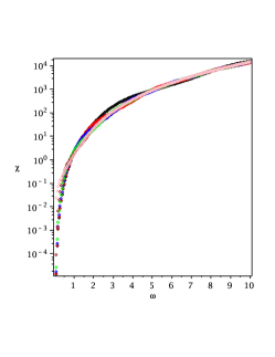
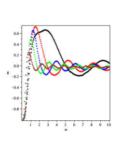
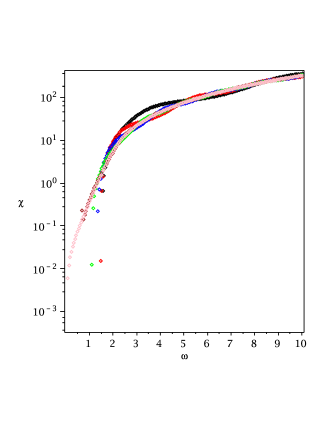
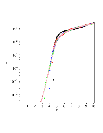
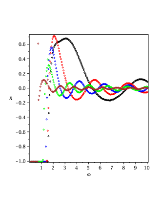
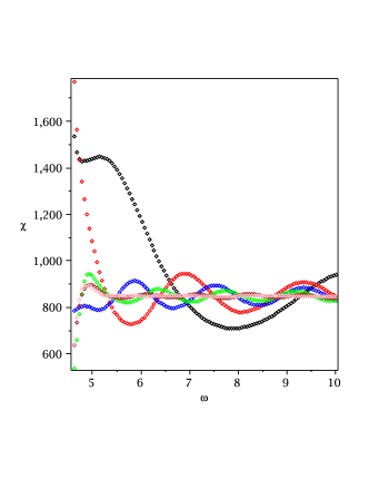
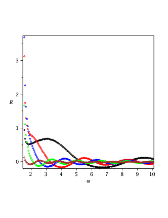
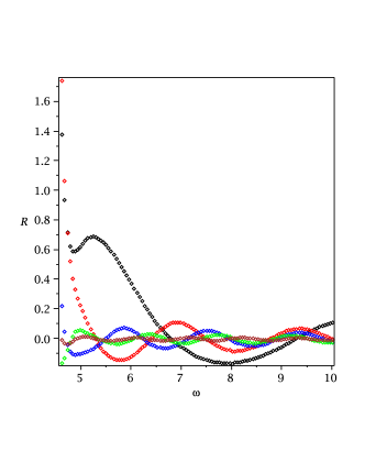
The spectral densities of the transverse stress are plotted at , and in Fig.2. Each plot includes five values of , corresponding to different stage of thermalization. The thermal spectral density of the transverse stress is also included for comparison. All the non-thermal spectral densities can be viewed as some oscillation on top of their thermal counterpart. The first period of oscillation occurs near #6#6#6Similar behavior is also observed in thermal spectral density[21, 22]. The oscillation damps in amplitude and grows in frequency as the medium thermalizes#7#7#7Here the frequency refers to the oscillation in spectral density. It is understood as the reciprocal of , i.e. approaches from below. This effect is clearly illustrated in Fig.3, where we plot the relative deviation .
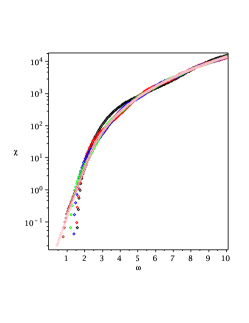
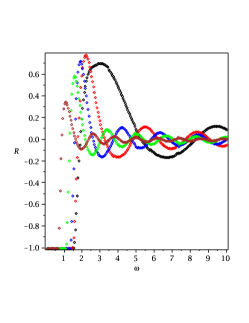
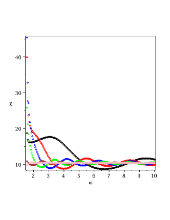
Parallel to the case of transverse stress, we also plot the spectral density of momentum density, at and in Fig.4 (The spectral density of momentum density at vanishes identically). Each plot include five values of , corresponding to different stage of thermalization.
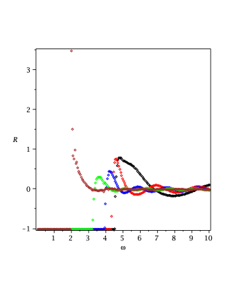
The relative deviation is plotted in Fig.5. We again observe the damping of amplitude and growing of frequency as the medium thermalizes.
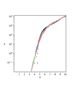
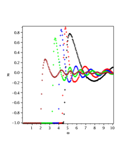
The spectral density of energy density, at and are plotted in Fig.6. (The spectral density of energy density again vanishes). Each plot includes five values of , corresponding to different stage of thermalization. The relative deviation is plotted in Fig.7. We find a very sharp peak in the first period of oscillation, which is removed from the final plot for a better comparison. We again confirm the non-thermal spectral density relaxes to thermal one in the qualitatively the same way as described in the previous cases.
In order to explain the observed phenomenon, we would like to obtain some analytical formula for the spectral density. This is possible in the final freezing stage, where there is a simple asymptotic ratio (33). To the leading order in , the boundary condition as is:
| (48) |
For the purpose of illuminating the problem, it is enough to focus on , the EOM of which has the simplest form. Its EOM (39) is solvable in terms of Heun function. However the property of Heun function is not fully understood.#8#8#8see [10] for a discussion. We have to use some approximation method, and in the regime of large the WKB treatment is appropriate . Following [26, 23], we obtain the expression of near the boundary up to normalization(see Appendix.A for details of the treatment):
| (55) |
where the constants are defined by:
| (56) |
The retarded correlator is calculated from the prescription (43). We have dropped an additional contact term: .
| (59) |
where we have defined .
In the large limit, the non-logarithmic term in the second case is exponentially suppressed. Therefore the lowest order result in agrees with the zero temperature one. [23]#9#9#9the imaginary part has an opposite sign, which is due to a different convention in Fourier transform. The higher order correction is due to the emergence of wave from the “horizon”. The phase difference between infalling and outfalling waves gives rise to the oscillating behavior in . We have also calculated (59), with numerically obtained and restored the contact term. The result show very good agreement with retarded correlator obtained in Sec.3.2 in region of large .
The physical interpretation of (59) is most clear at vanishing momentum, . The n-th order correction appears as
| (60) |
Combined with the ratio of (33), the n-th order correction can be written as
| (61) |
Recall the WKB solution of the incoming wave at :
| (62) |
Taking into account the time factor , we see is just the time for the wave to travel back-and-forth in WKB potential. We define the echo time
| (63) |
in which the wave makes a roundtrip. The n’th order correction to the two-point function (spectral density) has an echo time of , with a suppressed amplitude, obviously the -th echo.
This resembles the usual echo phenomenon with a sound reflected by a wall. Furthermore, the oscillations in spectral density as a function of frequency result, after the Fourier transform, in a as a function of time at the echo time. The peak is a result of many harmonics coherently added together: while smooth equilibrium spectral densities correspond to (thermally occupied) field harmonics which are completely incoherent to each other. We thus interpret “echo” as a partial re-appearance of coherence which was present in the original “color glass” fields at the collision moment. As the shell keeps falling toward the “horizon”, , the echo time tends to infinity and the medium loses all the coherence.
Although we derived it in near-thermal position of the shell, the echo phenomenon by itself is not restricted to the final freezing stage but exists throughout the whole process: its manifestation is in the spectral density of Fig.3, Fig.5 and Fig.7. Looking for “echo” in dynamical (time dependent) shell is perhaps worth addressing in later work.
3.3 Can the bounary observer see what happens below the shell?
In the rest of the paper we have chosen the boundary condition to correspond to the infalling wave at -infinity (the AdS center), which leads to the solution (30) and its consequences discussed above. This particular choice is natural in the standard setting, when all the probes (the source and the sink) sending gravitational wave the AdS boundary .
Now we switch to another issue: the gravitational wave emerging from inside, below the shell, . The motivation for studying this case is as follows. All stationary black hole metrics are such that no signal from the inside the horizon can propagate outside it: in particular, the geodesics do not cross horizon. But in the falling shell case we consider, the metric coincides with black hole one only above the shell, while inside it is the solution the horizon, since gravity of the shell produces no effect inside it. The question then is, can an observer on the boundary see what happens inside the shell?
Thus a wave sent from below would propagate all the way till the shell without any problems, and scatter on it. So we are looking now for a solution, which in the region inside the shell contains both outfalling and infalling waves, while outside () it has only outfalling wave propagating toward the boundary. At the shell the matching condition is again given by (3.1), and the precise relation between outfalling and infalling waves can be worked out parallel to what we did above. As always, a generic graviton is split into three channels, with the same eqns.
The gravitational wave outside the shell contains only the outfalling component. This is a solution in thermal-AdS metric which, if extrapolated to (non-existing) region would be originating from the horizon. Thus at it is , it is understood as the behavior since . The wave inside the shell can be written as:
| (64) |
With similar argument as before, we can approximate . Matching solutions at both sides and according to Israel condition (3.1.2), we obtain the asymptotic reflection ratio
| (65) |
which, at the shell approaching the horizon tends to zero. This means as the shell approaches the horizon, the portion of the wave reflected by the shell disappears, and thus all the wave emerging from below the shell is transmitted!
(To convince the reader that this conclusion is correct, here is another argument. As we have shown in the beginning of the paper, as the shell approach horizon one recovers the solution for the AdS-BH background (without any shell), with only the infalling waves on either side of the horizon without reflection (black horizon). The solution with only outfalling waves we are now describing is its complex conjugate.)
The conclusion that even at late time our collapsing shell is not that black as a horizon, as signals from inside the shell can be seen, look surprising and worrisome at first. Note however that these signals are both strongly red-shifted and exponentially delayed by the warping factor . As , both effects become infinitely strong, in practical sense precluding the boundary observer from seeing what happens below the shell.
4 Conclusion and Outlook
Continuing the line of research started by our papers I and II, we have built a gravitational collapse scenario, describing equilibration of conformal strongly coupled plasma in the AdS/CFT setting. Using a simplified geometry we approximated falling collision debris by a single flat shell or membrane, falling from its initial position (given by the saturation scale) to its horizon (given by the equilibrium temperature). The setting itself provides inequality between the two scales, satisfied at RHIC.
The main simplification of the paper is that this shell is - independent on our world 3 spatial coordinates. Therefore the overall solution of Einstein eqns reduces to two separate regions with well known AdS-BH and AdS metrics. The falling of the shell is time dependent, its equation of motion is determined by the Israel junction condition, which we solve and analyzed. We also determined how final temperature (horizon position) depends on initial scale and shell tension.
In statistical mechanics it is known that fluctuations at different scales are independent, and that long-range fluctuations (IR) need more time to be equilibrated than the short-range (UV) ones. With the AdS/CFT setting and our geometric simplification, this fact is taken to its perfect form. It is connected to the well known gravitational phenomenon: gravity of a sphere is independent on its size outside it, and is completely absent inside. In the equilibrating gauge theory it means that mean quantities at all scales above some (corresponding to sliding position of the shell) are as in equilibrium, while those below it are unaffected, being the same as in vacuum without any matter.
This is in the title. More specifically it means the following. In this geometry a “single point observer” – who is only able to measure the average density and pressure – would be driven to the conclusion that the matter is instantaneously equilibrated at times. However more sophisticated “two point observer” who is able to study correlation functions of stress tensors would be able to observe deviations from the thermal case. We computed them explicitly, calculating a number of spectral densities at various positions of the shell, corresponding (in quasi-static approximation) to different stages of equilibration.
The equilibration process can roughly be divided into three stages: the initial acceleration, intermediate relativistic falling and final near-horizon freezing. By studying the graviton probes corresponding to three different combinations of , we calculate the retarded correlators of on the AdS boundary, The matching condition of on the shell is given by a variation of Israel junction condition. In the quasi-static limit, we study the retarded correlator of all graviton probes. We have shown that the collapsing geometry correctly reproduces the AdS-BH limit: as the shell approaches the “horizon” the ratio of the infalling wave and outfalling wave tends to infinity. We further confirmed this by numerically study the spectral density for transverse stress, momentum density and energy density, which allows us to see deviations between geometry with shell and equilibrated one (AdS BH).
We find that the main deviation between the non-thermal and equilibrium spectral densities are some oscillations. As the time goes on and the shell is at the position closer and closer to the horizon, these oscillations become exponentially smaller in amplitude and higher in frequency, eventually disappearing in the equilibrium state. In this sense we get numerical control over the relaxation process. In the final freezing stage, when the membrane is close to the horizon, and in large regime, we even find analytical expressions for these deviations using the WKB method.
Oscillations in spectral densities as a function of frequency are further explained by the “echo” effect, producing peaks at certain “echo” times in the response functions. We expect at those times partial restoration of field coherence which was present at the initial time of the collision in system’s wave function. For the near equilibrated medium we have the echo time analytically, from the WKB solution. The echo time tends to infinity as the medium thermalizes.
The echo phenomenon arises from the phase coherence between infalling and outfalling waves in the bulk at certain times: we expect it to exist in all gauge theory with a gravity dual. It is also interesting to extend the current study to scalar probe and vector probe. One can further study the effect of echo on electromagnetic () spectral densities related to production spectra [27] which can be observable in collisions.
An attentive reader will notice that apart of small discussion of upward moving waves, we we have not yet addressed the dynamics of the horizon formation, deferred for later studies. When this paper were near-completed, we learned about an interesting work by Hubeny,Liu and Rangamani [15] who discuss certain null geodesics related observation points at the boundary. Since phases of the waves add coherently near geometric optics paths (null geodesics), this is another interesting form of coherence, although perhaps unrelated to our WKB “echos”.
Finally, one may now think about relaxing our main assumption – flatness of the shell, e.g. by including first corrections resulting from slow variations of its position. In this case the metric above the shell would become time-dependent, allowing a “single point observer” to see some relaxation dynamics as well.
5 Acknowledgment
The work is partially supported by the US-DOE grants DE-FG02-88ER40388 and DE-FG03-97ER4014. S.L. would like to thank Keun-young Kim, Peng Dai, Yu-tin Huang and Elli Pomoni for multiple discussions.
Appendix A WKB treatment of (39)
In order to apply WKB method to (39), we need to convert it Schrodinger- type equation. Introducing a new field , (39) becomes:
| (66) |
with . is a large parameter to justify WKB. There are two singularities in (66): ,. The term proportional to may vanish at if . We discuss two cases separately: I , II and focus on only. The solution for can be obtained easily from the solution for by the substitution .
Case I : Away from the singularities, the WKB solution to (66) is given as:
| (67) |
with
Near the singularities, (66) becomes:
| (68) |
On the other hand, we have:
| (69) |
Matching the WKB solution with the approximate solutions near the singularities (using asymptotic expansion of Hankel function), we obtain:
| (70) |
Case.II : This case is a little more complicated because WKB approximation breaks down near . Away from , we have the following WKB solutions:
| (71) |
where ,.
We first match WKB solutions at . Near , (66) becomes:
| (72) |
where ,
(72) can be solved by Airy functions:
| (73) |
Using the asymptotic expansion of Airy functions:
| (74) |
We obtain the following match between WKB solutions:
| (75) |
Next we match WKB solutions with approximate solutions near singularities similarly as case I. Finally we have:
| (76) |
with ,
Summarizing all cases, we have:
| (83) |
Appendix B Gauge Choice for the Sound Channel
The aim of the section is to show it is possible render the following matching condition by a proper choice of gauge:
| (84) |
| (85) |
where all the quantities are evaluated at .
We note the residue gauge degree of freedom implies that it is sufficient to satisfy (3.1) up to a gauge choice. In particular, we could add pure gauge solution to the sound channel: inside the shell and outside. According to [24], the only pure gauge solution that touch ( with ) is:
| (86) |
Now, it is enough to satisfy:
| (87) |
where and . It is easy to see it is always possible to satisfy (B) with a proper choice of constants and .
References
- [1] J. M. Maldacena, Adv. Theor. Math. Phys. 2, 231 (1998) [Int. J. Theor. Phys. 38, 1113 (1999)] [arXiv:hep-th/9711200].
- [2] D. Teaney, J. Lauret and E. V. Shuryak, arXiv:nucl-th/0110037.
- [3] P. F. Kolb and U. W. Heinz, arXiv:nucl-th/0305084.
- [4] E. Shuryak, arXiv:0807.3033 [hep-ph].
- [5] S. Lin and E. Shuryak, Phys. Rev. D 77, 085013 (2008) [arXiv:hep-ph/0610168].
- [6] S. Lin and E. Shuryak, Phys. Rev. D 77, 085014 (2008) [arXiv:0711.0736 [hep-th]].
- [7] R. Venugopalan, arXiv:0806.1356 [hep-ph].
- [8] G. T. Horowitz and V. E. Hubeny, Phys. Rev. D 62, 024027 (2000) [arXiv:hep-th/9909056].
- [9] P. K. Kovtun and A. O. Starinets, Phys. Rev. D 72, 086009 (2005) [arXiv:hep-th/0506184].
- [10] A. Nunez and A. O. Starinets, Phys. Rev. D 67, 124013 (2003) [arXiv:hep-th/0302026].
- [11] A. O. Starinets, Phys. Rev. D 66, 124013 (2002) [arXiv:hep-th/0207133].
- [12] U. H. Danielsson, E. Keski-Vakkuri and M. Kruczenski, Nucl. Phys. B 563, 279 (1999) [arXiv:hep-th/9905227].
- [13] U. H. Danielsson, E. Keski-Vakkuri and M. Kruczenski, JHEP 0002, 039 (2000) [arXiv:hep-th/9912209].
- [14] S. B. Giddings and A. Nudelman, JHEP 0202, 003 (2002) [arXiv:hep-th/0112099].
- [15] V. E. Hubeny, H. Liu and M. Rangamani, JHEP 0701, 009 (2007) [arXiv:hep-th/0610041].
- [16] K. S. . Thorne, R. H. . Price and D. A. . Macdonald, NEW HAVEN, USA: YALE UNIV. PR. (1986) 367p
- [17] W. Israel, Nuovo Cim. B 44S10, 1 (1966) [Erratum-ibid. B 48, 463 (1967 NUCIA,B44,1.1966)].
- [18] R. Venugopalan, Eur. Phys. J. C 43, 337 (2005) [arXiv:hep-ph/0502190].
- [19] E. Shuryak, S. J. Sin and I. Zahed, J. Korean Phys. Soc. 50, 384 (2007) [arXiv:hep-th/0511199].
- [20] G. Policastro, D. T. Son and A. O. Starinets, JHEP 0209, 043 (2002) [arXiv:hep-th/0205052].
- [21] P. Kovtun and A. Starinets, Phys. Rev. Lett. 96, 131601 (2006) [arXiv:hep-th/0602059].
- [22] S. A. Hartnoll and S. Prem Kumar, JHEP 0512, 036 (2005) [arXiv:hep-th/0508092].
- [23] D. T. Son and A. O. Starinets, JHEP 0209, 042 (2002) [arXiv:hep-th/0205051].
- [24] G. Policastro, D. T. Son and A. O. Starinets, JHEP 0212, 054 (2002) [arXiv:hep-th/0210220].
- [25] D. Z. Freedman, S. D. Mathur, A. Matusis and L. Rastelli, Nucl. Phys. B 546, 96 (1999) [arXiv:hep-th/9804058].
- [26] D. Teaney, Phys. Rev. D 74, 045025 (2006) [arXiv:hep-ph/0602044].
- [27] S. Caron-Huot, P. Kovtun, G. D. Moore, A. Starinets and L. G. Yaffe, JHEP 0612, 015 (2006) [arXiv:hep-th/0607237].