Berezinskii-Kosterlitz-Thouless transition in trapped quasi-two-dimensional Fermi gas near a Feshbach resonance

Abstract

We study the superfluid transition in a quasi-two-dimensional Fermi gas with a magnetic field tuning through a Feshbach resonance. Using an effective two-dimensional Hamiltonian with renormalized interaction between atoms and dressed molecules, we investigate the Berezinskii-Kosterlitz-Thouless transition temperature by studying the phase fluctuation effect. We also take into account the trapping potential in the radial plane, and discuss the number and superfluid density distributions. These results can be compared to experimental outcomes for gases prepared in one-dimensional optical lattices.

I Introduction

The study of superfluidity and superconductivity in two-dimensional (2D) Fermi systems has attracted great attention in the past several decades, partly because of its close relationship to the problem of high-$T_{c}$ superconductors anderson-88 ; sachdev-03 . Recently, the experimental progress on creating quasi-low-dimensional atomic gases in optical lattices modugno-03 ; moritz-05 ; stoferle-06 ; chin-06 ; lewenstein-07 and on atom chips aubin-06 ; fotagh-07 provides us a possibility of realizing and studying superfluidity in a more controllable platform. In particular, with the aid of tuning an external magnetic field through a Feshbach resonance, the interaction between fermionic atoms can be tuned continuously from the Bardeen-Cooper-Schrieffer (BCS) limit to the Bose-Einstein condensation (BEC) limit, so that the BCS-BEC crossover can be studied crossover .

The BCS-BEC crossover in a 2D Fermi system has been discussed at both zero randeria-90 and finite temperatures gusynin-99 ; botelho-06 , where an effective 2D Hamiltonian with atom-atom interaction (called model 1) is employed. However, for strongly interacting fermionic atoms in a realistic quasi-2D geometry, due to the inevitable population of many excited levels along the strongly confined transverse direction kestner-06 , one needs to introduce a composite particle called dressed molecule to account for the population in these transverse excited levels, and write down a more complicated form for the effective 2D Hamiltonian (called model 2) with renormalized interaction between atoms (in the transverse ground level) and dressed molecules kestner-07 . We have shown that the model 1 and the model 2 Hamiltonians lead to qualitatively distinct results in some cases zhang-08 . For instance, for quasi-2D fermions in a weak global harmonic trap, the model 1 Hamiltonian predicts a constant value of the Thomas-Fermi cloud size at zero temperature from the BCS to the BEC limit. In contrast, the model 2 Hamiltonian predicts that the cloud size shrinks as one approaches the BEC limit zhang-08 , which is the correct trend as one should expect from the BCS-BEC crossover picture.

In this paper, we extend the discussion of the model 2 Hamiltonian to finite temperatures by taking into account the fluctuation effects. In particular, we consider a trapped quasi-2D Fermi gas and study the superfluid transition temperature across a wide range of Feshbach resonance. Note that according to the Mermin-Wagner-Hohenberg-Coleman theorem MWHC , phase fluctuations are dramatic at any finite temperatures such that there will be no ordinary long-range order in two dimensions. In this case, the superfluid transition is not accompanied by a Bose condensation, but instead characterized by a Berezinskii-Kosterlitz-Thouless (BKT) type, for which the vortex-antivortex pairs start to form at the transition and a topological order is established BKT . Using the model 2 Hamiltonian, we show that in a uniform quasi-2D Fermi gas, the BKT transition temperature $T_{\mathrm{BKT}}$ increases from zero at the BCS limit and approaches monotonically to almost a constant value about $0.075E_{F}$ at the BEC limit, where $E_{F}$ is the 2D Fermi energy. Furthermore, we take into account the weak harmonic trap in the radial plane, and investigate the number and superfluid density distributions under the local density approximation (LDA). As a characteristic feature of a BKT transition, a finite jump of superfluid density is present in the middle of the trap, which takes a universal value of $2T_{\rm BKT}/\pi$ nelson-77 .

II Formulation

A quasi-2D Fermi gas is typically prepared in experiments by means of a one-dimensional (1D) deep optical lattice along the axial ($z$) direction, where tunneling between different lattice sites is completely suppressed. A 1D lattice is described by the potential $V_{\mathrm{ol}}=-V_{0}\exp[-2(x^{2}+y^{2})/w^{2}]\cos(k_{z}z)$, where $k_{z}$ is the wave vector of the laser beam, and $w$ is the waist width satisfying $w\gg k_{z}^{-1}$. This optical lattice potential can be approximated around the minimal points by a strongly anisotropic pancake-shaped harmonic potential with $V\approx m(\omega_{z}z^{2}+\omega_{\perp}r^{2})/2$, where $\omega_{z}=\sqrt{V_{0}k_{z}^{2}/m}$, $\omega_{\perp}=2\sqrt{V_{0}/(mw^{2})}$, and $r=\sqrt{x^{2}+y^{2}}$ is the radial distance. The strong anisotropy of the trap ($\omega_{z}\gg\omega_{\perp}$) introduces two well separated energy scales, which allows us to first deal with the axial degrees of freedom by deriving an effective 2D Hamiltonian, while the radial degrees of freedom are left for later treatment with the LDA approximation.

The effective 2D Hamiltonian describing a quasi-2D Fermi gas within a strongly axial confinement is derived in Ref. kestner-07 . Under natural units ($\hbar=k_{B}=1$), the Hamiltonian takes the form

$$\mathcal{H} = \sum_{\mathbf{k},\sigma}\left(\epsilon_{\mathbf{k}}-\mu\right)a_{\mathbf{k},\sigma}^{\dagger}a_{\mathbf{k},\sigma}+\sum_{\mathbf{q}}\left(\frac{\epsilon_{\mathbf{q}}}{2}+\lambda_{b}-2\mu\right)d_{\mathbf{q}}^{\dagger}d_{\mathbf{q}}$$ (1)

$$+ \frac{\alpha_{b}}{L}\sum_{\mathbf{k},\mathbf{q}}\left(a_{\mathbf{k},\uparrow}^{\dagger}a_{-\mathbf{k}+\mathbf{q},\downarrow}^{\dagger}d_{\mathbf{q}}+h.c.\right)$$

$$+ \frac{V_{b}}{L^{2}}\sum_{\mathbf{k},\mathbf{k^{\prime}},\mathbf{q}}a_{\mathbf{k},\uparrow}^{\dagger}a_{-\mathbf{k}+\mathbf{q},\downarrow}^{\dagger}a_{-\mathbf{k^{\prime}},\downarrow}a_{\mathbf{k^{\prime}}+\mathbf{q},\uparrow},$$

where $a_{\mathbf{k},\sigma}$ and $d_{\mathbf{q}}$ are the annihilation operators for fermionic atoms and bosonic dressed molecules, respectively. The dressed molecule consists of a tight pair of atoms distributed in the transverse (axial) excited levels as well as the population in the closed Feshbach channel kestner-07 . In Eq. (1), $\epsilon_{\mathbf{k}}=\mathbf{k}^{2}/(2m)$ is the dispersion relation for fermions with mass $m$ and radial momentum $\mathbf{k}=(k_{x},k_{y})$, $\mu$ is the fermionic chemical potential, $\sigma=\uparrow,\downarrow$ labels the pseudo-spin, and $L^{2}$ is the quantization area. In the remainder of this manuscript, we choose $\omega_{z}$ as the energy unit so that $\mathcal{H}$, $\mu$, and $\epsilon_{\mathbf{k}}=a_{z}^{2}\mathbf{k}^{2}/2$ become dimensionless, where $a_{z}\equiv\sqrt{1/(m\omega_{z})}$ is the characteristic length scale for axial motion.

The 2D effective bare parameters $\lambda_{b}$ (detuning), $\alpha_{b}$ (atom-molecule coupling rate), and $V_{b}$ (background interaction) in Eq. 1 are connected with the 2D physical parameters $\lambda_{p}$, $\alpha_{p}$, and $V_{p}$ through the renormalization relation

$$\left[V_{p}^{\text{eff}}(x)\right]^{-1} \equiv \left[V_{p}+\frac{\alpha_{p}^{2}}{x-\lambda_{p}}\right]^{-1}$$ (2)

$$= \left[V_{b}+\frac{\alpha_{b}^{2}}{x-\lambda_{b}}\right]^{-1}+\frac{1}{L^{2}}\sum_{\mathbf{k}}\frac{1}{2\epsilon_{\mathbf{k}}+\omega_{z}},$$

which is an identity for the variable $x$. The inverse of the physical effective interaction $\left[V_{p}^{\text{eff}}(x)\right]^{-1}$ are determined from the three-dimensional (3D) atomic scattering data through kestner-07

$$\left[V_{p}^{\text{eff}}(x)\right]^{-1}=\frac{\sqrt{2\pi}}{a_{z}^{2}}\left[\left(U_{p}+\frac{g_{p}^{2}}{x-\gamma_{p}}\right)^{-1}-S_{p}(x)+\sigma_{p}(x)\right],$$ (3)

where $U_{p}=4\pi a_{bg}/a_{z}$, $g_{p}^{2}=\mu_{co}WU_{p}/\omega_{z}$, and $\gamma_{p}=\mu_{co}(B-B_{0})/\omega_{z}$ are 3D dimensionless parameters. Here, $a_{bg}$ is the background scattering length, $\mu_{co}$ is the difference in magnetic moments between the open and closed collision channels, $W$ is the resonance width, and $B_{0}$ is the resonance point. The functions in Eq. (3) are kestner-07

$$S_{p}(x) \equiv \frac{1}{\sqrt{32}\pi}\int_{0}^{\infty}ds\left[\frac{\Gamma(s-x/2)}{\Gamma(s+1/2-x/2)}-\frac{1}{\sqrt{s}}\right],$$ (4)

$$\sigma_{p}(x) \equiv \frac{\ln\left|x\right|}{4\pi\sqrt{2\pi}},$$ (5)

where $\Gamma(x)$ is the gamma function.

The partition function $\mathcal{Z}$ of the Hamiltonian Eq. (1) at temperature $T=\beta^{-1}$ can be expressed as an imaginary-time functional integral with action

$$S=\int_{0}^{\beta}d\tau\left[\sum_{\mathbf{k,\sigma}}a_{\mathbf{k},\sigma}^{\dagger}\partial_{\tau}a_{\mathbf{k},\sigma}+\sum_{\mathbf{q}}d_{\mathbf{q}}^{\dagger}\partial_{\tau}d_{\mathbf{q}}+\mathcal{H}\right],$$ (6)

where $a_{\mathbf{k},\sigma}=a_{\mathbf{k},\sigma}(\tau)$ and $d_{\mathbf{q}}=d_{\mathbf{q}}(\tau)$ become imaginary time dependent variables. By introducing the Hubbard-Stratonovich field $b_{\mathbf{q}}(\tau)$, which couples to $a^{\dagger}a^{\dagger}$, and integrating out the fermions, we obtain $\mathcal{Z}=\int\mathcal{D}[b^{\dagger},b,d^{\dagger},d]\exp(-S_{\mathrm{eff}})$, with the effective action given by

$$S_{\mathrm{eff}} = \int_{0}^{\beta}d\tau\sum_{\mathbf{q}}\bigg{[}-\frac{|b_{\mathbf{q}}(\tau)|^{2}L^{2}}{V_{b}}-\mu$$ (7)

$$+d_{\mathbf{q}}^{\dagger}(\tau)\left(\partial_{\tau}+\frac{\epsilon_{\mathbf{q}}}{2}+\lambda_{b}-2\mu\right)d_{\mathbf{q}}(\tau)\bigg{]}-\mathbf{Tr}\left[\ln\mathbf{G}_{\mathbf{k},\mathbf{k}^{\prime}}^{-1}\right].$$

Notice that the trace $\mathbf{Tr}$ is taken over momentum, imaginary time, and Nambu indices of the inverse Nambu matrix $\mathbf{G}^{-1}$, with

$$\mathbf{G}_{\mathbf{k},\mathbf{k}^{\prime}}^{-1}=\left(\begin{array}[]{cc}-(\partial_{\tau}+\epsilon_{\mathbf{k}}-\mu)\delta_{\mathbf{k},\mathbf{k}^{\prime}}&-\Delta_{\mathbf{k}-\mathbf{k}^{\prime}}(\tau)\\ -\Delta_{\mathbf{k}-\mathbf{k}^{\prime}}^{\dagger}(\tau)&-(\partial_{\tau}-\epsilon_{\mathbf{k}}+\mu)\delta_{\mathbf{k},\mathbf{k}^{\prime}}\end{array}\right).$$ (8)

Here, $\Delta_{\mathbf{q}}(\tau)\equiv(\alpha_{b}/L)d_{\mathbf{q}}(\tau)+b_{\mathbf{q}}(\tau)$ is the field whose stationary value corresponds to the order parameter.

We expand the action around a stationary and homogeneous saddle point $\Delta_{0}\equiv(\alpha_{b}/L)d_{0}+b_{0}$. The saddle point equation is derived from the saddle point action $S_{0}[\Delta_{0}]$ via the stationary conditions $\delta S_{0}/\delta\Delta_{0}=0$. This process leads to

$$\left[V_{p}^{\text{eff}}(2\mu)\right]^{-1}=-\frac{1}{L^{2}}\sum_{\mathbf{k}}\left[\frac{1}{2E_{\mathbf{k}}}\tanh\left(\frac{\beta E_{\mathbf{k}}}{2}\right)-\frac{1}{2\epsilon_{\mathbf{k}}+1}\right],$$ (9)

where $E_{\mathbf{k}}=\sqrt{(\epsilon_{\mathbf{k}}-\mu)^{2}+\Delta_{0}^{2}}$ is the quasi-particle excitation spectrum. We have used the 2D renormalization relation Eq. (2) in the derivation, which introduces the term $1/(2\epsilon_{\mathbf{k}}+1)$.

In order to study the fluctuation around the saddle points of $d_{0}$, $b_{0}$, and $\Delta_{0}$, we next write the field operators as

$$d_{\mathbf{q}}(\tau) = \left(|d_{0}|+\delta|d_{\mathbf{q}}(\tau)|\right)e^{i\phi_{\mathbf{q}}(\tau)},$$ (10a)

$$b_{\mathbf{q}}(\tau) = \left(|b_{0}|+\delta|b_{\mathbf{q}}(\tau)|\right)e^{i\eta_{\mathbf{q}}(\tau)},$$ (10b)

$$\Delta_{\mathbf{q}}(\tau) = \left(|\Delta_{0}|+\delta|\Delta_{\mathbf{q}}(\tau)|\right)e^{i\theta_{\mathbf{q}}(\tau)},$$ (10c)

which are all assumed to be slowly varying in both spatial and temporal coordinates. Here, $\delta|d_{\mathbf{q}}|$, $\delta|b_{\mathbf{q}}|$, and $\delta|\Delta_{\mathbf{q}}|$ are magnitude fluctuations, while $\phi_{\mathbf{q}}$, $\eta_{\mathbf{q}}$, and $\theta_{\mathbf{q}}$ are phase fluctuations. The magnitude fluctuations correspond to gapped excitations, whose contribution can be neglected. However, the phase fluctuations correspond to gapless excitations, and it is their presence that breaks the ordinary long-range order in two dimensions. Notice that since the order parameter $\Delta_{\mathbf{q}}$ is a linear combination of $d_{\mathbf{q}}$ and $b_{\mathbf{q}}$, neglecting its magnitude fluctuation $\delta|\Delta_{\mathbf{q}}|$ is equivalent to assuming a same phase factor for $d_{\mathbf{q}}$ and $b_{\mathbf{q}}$. We thus have

$$\phi_{\mathbf{q}}(\tau)\equiv\eta_{\mathbf{q}}(\tau)\equiv\theta_{\mathbf{q}}(\tau).$$ (11)

The phase fluctuation $\theta_{\mathbf{q}}(\tau)$ around the saddle points is in general not a small value, so the phase factor in the order parameter cannot be directly expanded, but must be treated as a whole. This can be done by introducing a unitary transformation ${\hat{\mathcal{U}}}\mathcal{O}\equiv\exp[i\theta_{\mathbf{q}}(\tau)/2]\mathcal{O}$ for the fields $\mathcal{O}=d_{\mathbf{q}}$, $b_{\mathbf{q}}$, and $\Delta_{\mathbf{q}}$. As a result of this transformation, and after a Fourier transformation back to the coordinate space, we can expand the effective action around its stationary point of $\Delta_{0}$, leading to

$$S_{\mathrm{eff}}=S_{0}[\Delta_{0}]+S_{\mathrm{fluc}}[\nabla\theta,\partial_{\tau}\theta],$$ (12)

where the fluctuation contribution $S_{\mathrm{fluc}}$ contains terms only involving spatial or temporal gradients of the field $\theta$, which are assumed to be small.

Expanding $S_{\mathrm{fluc}}$ up to the quadratic order of $\nabla\theta$ and $\partial_{\tau}\theta$ leads to

$$S_{\mathrm{fluc}}\approx\frac{1}{2}\int_{0}^{\beta}d\tau\int d^{2}\mathbf{r}\left[iJ\partial_{\tau}\theta+K(\partial_{\tau}\theta)^{2}+\rho_{s0}(\nabla\theta)^{2}\right],$$ (13)

where $\rho_{s0}$ represents the phase stiffness (or called the superfluid density) and takes the form

$$\rho_{s0} = \frac{1}{4m}\Bigg{\{}2n_{b}+\frac{1}{L^{2}}\sum_{\mathbf{k}}\left[1-\frac{\epsilon_{\mathbf{k}}}{E_{\mathbf{k}}}\tanh\left(\frac{\beta E_{\mathbf{k}}}{2}\right)\right]$$ (14)

$$\hskip 28.45274pt-\frac{\beta\hbar^{2}}{4mL^{2}}\sum_{\mathbf{k}}k^{2}\mathrm{sech}^{2}\left(\frac{\beta E_{\mathbf{k}}}{2}\right)\Bigg{\}}.$$

Here, $n_{b}=\Delta^{2}\partial[V_{p}^{\text{eff}}(2\mu)]^{-1}/\partial\mu$ denotes the dressed-molecular population. Other parameters in Eq. (13) are

$$J = 2n_{b}-\frac{1}{L^{2}}\sum_{\mathbf{k}}\frac{\epsilon_{\mathbf{k}}-\mu}{E_{\mathbf{k}}}\tanh\left(\frac{\beta E_{\mathbf{k}}}{2}\right),$$ (15)

$$K = \frac{m}{8\pi}\left[1+\frac{\mu}{\sqrt{\mu^{2}+\Delta_{0}^{2}}}\tanh\left(\frac{\beta\sqrt{\mu^{2}+\Delta_{0}^{2}}}{2}\right)\right].$$ (16)

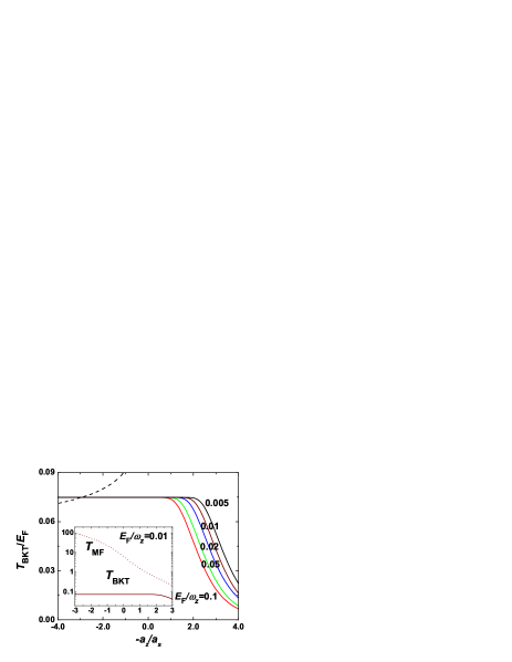
Figure 1: (Color online) Superfluid transition temperature $T_{\mathrm{BKT}}$ (solid lines) of a uniform quasi-2D Fermi gas for various values of $E_{F}/\omega_{z}$. Notice that $T_{\mathrm{BKT}}$ increases monotonically from the BCS (right) to the BEC (left) side of the resonance, and approaches to a limiting value of $\sim 0.075E_{F}$. In the BEC limit, $T_{\rm BKT}$ can also be estimated by considering a weakly interacting gas of composite bosons with 3D scattering length of $0.6a_{s}$, leading to a logarithmically varying result (dashed line). The mean-field transition temperature $T_{\mathrm{MF}}$ (dashed line in the inset) is also shown as a comparison for $E_{F}/\omega_{z}=0.01$.

By decomposing the phase fluctuation $\theta(\mathbf{r},\tau)=\theta_{v}(\mathbf{r},\tau)+\theta_{\mathrm{sw}}(\mathbf{r},\tau)$ into a vortex part $\theta_{v}$ and a vortex-free spin-wave part $\theta_{\mathrm{sw}}$, one can separate the effective action $S_{\mathrm{eff}}$, and hence the thermodynamic potential as botelho-06

$$\Omega=\frac{S_{\mathrm{eff}}}{\beta}=\Omega_{0}+\Omega_{v}+\Omega_{\mathrm{sw}},$$ (17)

where $\Omega_{0}$, $\Omega_{v}$ and $\Omega_{\mathrm{sw}}$ are the corresponding contributions from the saddle point action $S_{0}$, the vortex contribution from $\theta_{v}$, and the spin-wave contribution from $\theta_{\mathrm{sw}}$, respectively. The spin-wave part can be integrated out to give $\Omega_{\mathrm{sw}}=T\sum_{\mathbf{k}}\ln\left(1-e^{-ck/T}\right)$, where $c=\sqrt{\rho_{s0}/J}$ is the speed of the spin-wave. The number equation hence can be obtained via $N=-\partial\Omega/\partial\mu$, leading to

$$n = \frac{N}{L^{2}}=n_{\mathrm{sw}}+2n_{b}$$ (18)

$$+\frac{1}{L^{2}}\sum_{\mathbf{k}}\left[1-\frac{\epsilon_{\mathbf{k}}}{E_{\mathbf{k}}}\tanh\left(\frac{\beta E_{\mathbf{k}}}{2}\right)\right]$$

with the spin-wave contribution $n_{\mathrm{sw}}=-\partial\Omega_{\mathrm{sw}}/\partial\mu$. By writing the number equation as above, we implicitly assume a vanishingly small vortex density, such that the vortex contribution to the number equation can be safely neglected. This condition is in general valid for temperatures around or below the superfluid transition temperature minnhagen-87 .

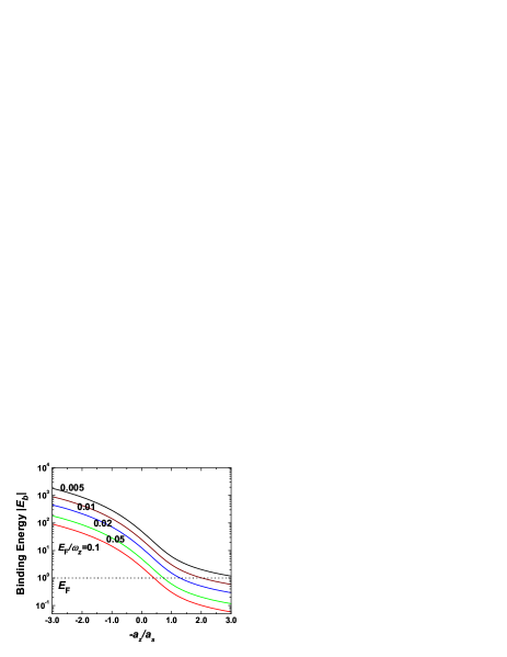
Figure 2: (Color online) Two-body binding energy $|E_{b}|$ (solid lines) as a function of $a_{z}/a_{s}$ for various values of $E_{F}/\omega_{z}$. Notice that $|E_{b}|$ can exceed $E_{F}$ (dotted) even on the high-field side of the resonance point, hence pushes the system into the BEC limit as indicated by the transition temperature shown in Fig. 1.

The $\rho_{s0}$ is the superfluid density at the microscopic scale, and the vortex fluctuation tends to renormalize (decrease) the superfluid density when the physical scale $l$ goes up. When the superfluid density is renomalized to zero with $l\rightarrow\infty$, the Berezinskii-Kosterlitz-Thouless (BKT) transition takes phase where the system changes from a superfluid phase to a normal phase. The renormalization-group (RG) flow depends on the vortex core energy $E_{c}$, which can be estimated by $E_{c}=0.78\pi\rho_{s0}$ minnhagen-85 . The RG equations for the superfluid density $\rho_{s}$ and the fugacity $y=e^{-\beta E_{c}}$ are given by kosterlitz-74

$$\frac{dK^{-1}(l)}{dl} = 4\pi^{3}y^{2}(l)+O(y^{3}),$$ (19)

$$\frac{dy(l)}{dl} = \left[2-\pi K(l)\right]y(l)+O(y^{2}),$$ (20)

where $K(l)\equiv\rho_{s}(l)/T$. The initial conditions are $\rho_{s}(l=0)=\rho_{s0}$ and $y(l=0)=\exp(-\pi\rho_{s0}/2T)$. The fixed point $(y(\infty),K(\infty))=(0,2/\pi)$ of these RG equations corresponds to the critical condition for the BKT transition, where the vortex- antivortex pairs start to dissociate and break superfluidity. Thus, the equation for the critical temperature $T_{c}=T_{\mathrm{BKT}}$ is determined as kosterlitz-74

$$T_{\mathrm{BKT}}=\frac{\pi}{2}\rho_{s}^{R},$$ (21)

where $\rho_{s}^{R}=\lim_{l\rightarrow\infty}\rho_{s}(l)$ is the renormalized superfluid density. This equation must be solved together with the saddle-point equation (9), the number equation (18), and the RG equations (19) and (20) to determine $\mu$, $\Delta_{0}$, and $T_{\mathrm{BKT}}$ as functions of the magnetic field detuning. As a comparison, the mean-field transition temperature $T_{\mathrm{MF}}$ can be calculated by solving only Eqs. (9) and (18) with $\Delta_{0}=0$. Next, we will consider some specific systems and discuss the corresponding numerical results.

III Numerical results

We first ignore the trapping potential in the radial plane, and consider a uniform quasi-2D Fermi gas. A typical set of results of $T_{\mathrm{BKT}}$ for various values of $\omega_{z}$ are shown in Fig. 1. Here, we consider the case of ⁶Li and use the parameters $a_{bg}=-1405a_{0}$, $W=300$ G, and $\mu_{co}=2\mu_{B}$, where $a_{0}$ and $\mu_{B}$ are Bohr radius and Bohr magneton, respectively. We also notice that when plotted as functions of the inverse 3D scattering length $a_{z}/a_{s}$, the results for ⁴⁰K are very close to those for ⁶Li, indicating the universal behavior around the resonance point.

Notice that the superfluid transition temperature $T_{\mathrm{BKT}}$ increases continuously from the BCS to the BEC side of the Feshbach resonance, and saturates to a limiting value of $T_{\mathrm{BKT}}\approx 0.075E_{F}$. This limiting value of $T_{\mathrm{BKT}}$ is expected for $\rho_{s0}\approx n/(4m)$, which corresponds to the BEC limit of a quasi-2D Fermi gas where paired fermions behave like weakly interacting bosons with number density $n/2$ and mass $2m$. In the BEC limit, we can also consider the particles as composite bosons with effective three-dimensional scattering length of $0.6a_{s}$ petrov-04 . For weakly interacting bosons, more accurate results are available for the BKT transition temperature based on a combination of the quantum Monte Carlo simulation prokofev-01 and the renormalization group approach holzmann-07 , which predicts that $T_{\mathrm{BKT}}$ goes down logarithmically with the scattering length. This more accurate result in the BEC limit is also shown in Fig. 1, which is slightly deviant from our fermionic calculation.

We note also from Fig. 1 that the BEC limit value of $T_{\mathrm{BKT}}$ can even be reached on the BCS side of the Feshbach resonance (with $a_{s}<0$). In fact, since a two-body bound state is always present in quasi-low dimensions at arbitrary detunings, the BEC limit of a quasi-2D Fermi gas can be realized as long as the condition $|E_{b}|\gg E_{F}$ is satisfied, regardless of the sign of the 3D scattering length $a_{s}$. This property is in clear contrast to the 3D case, where a bound state is only present with positive $a_{s}$, hence the BEC limit can only be realized on the low-field side of a Feshbach resonance. Here, the two-body binding energy $|E_{b}|$ is determined by solving the Hamiltonian (1) for two particles, which gives

$$\left[V_{p}^{\text{eff}}(E_{b})\right]^{-1}=\frac{1}{4\pi a_{z}^{2}}\ln(-E_{b}).$$ (22)

The corresponding results for $|E_{b}|$ are plotted in Fig. 2. Notice that for the case with $E_{F}/\omega_{z}=0.005$, the binding energy $|E_{b}|\approx 2.0E_{F}$ for $a_{z}/a_{s}\approx-2.0$, leading to a BKT transition temperature of the BEC limit value $T_{\mathrm{BKT}}\approx 0.075E_{F}$, as shown in Fig. 1.

Another feature of Fig. 1 is that the transition temperature $T_{\mathrm{BKT}}$ increases with the axial trapping frequency $\omega_{z}$ at a fixed detuning. This trend can also be easily understood by analyzing the two-body binding energy $|E_{b}|$. In fact, at a given detuning, $|E_{b}|$ increases with $\omega_{z}$ as shown in Fig. 2, hence pushes the quasi-2D system further to the BEC limit.

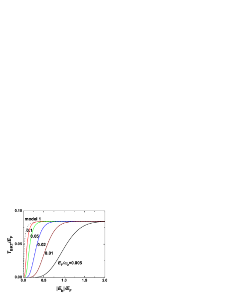
Figure 3: (Color online) Superfluid transition temperature $T_{\mathrm{BKT}}$ (solid lines) plotted as functions of the two-body binding energy $|E_{b}|$. The results are compared with the outcome of an effective 2D Hamiltonian with renormalized atom-atom interaction (model 1, dotted line), which is discussed in Refs. gusynin-99 ; botelho-06 .

The results of $T_{\mathrm{BKT}}$ should also be compared with the outcome of an effective 2D Hamiltonian with renormalized atom-atom interaction (model 1), which is discussed in Refs. gusynin-99 ; botelho-06 . In Fig. 3, we show $T_{\mathrm{BKT}}$ calculated using both models as functions of the binding energy $|E_{b}|$. One prediction of the model 1 is that the many-body physics (such as the BKT transition temperature) takes a universal behavior, which only depends on the two-body binding energy $|E_{b}|$ in the unit of $E_{F}$ randeria-90 ; gusynin-99 ; botelho-06 . As shown in Fig. 3, this is clearly not the case for the results from the model 2, where the transition temperature $T_{\mathrm{BKT}}$ also depends on the other energy scale such as the transverse trapping frequency $\omega_{z}$. Notice that both of the models predict roughly the same limiting value of $T_{\mathrm{BKT}}$ for large values of $|E_{b}|$ (in the BEC limit), since in that limit the system behaves like weakly interacting bosons, and $T_{\mathrm{BKT}}$ gets very insensitive to the interaction between these composite bosons (logarithmic dependence as mentioned above).

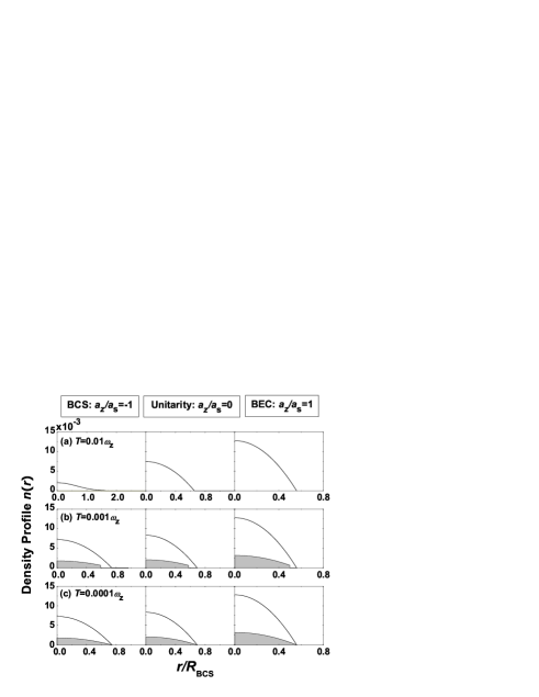
Figure 4: (Color online) In-trap number (solid) and superfluid (shaded area) density distributions at (a) $T=0.01\omega_{z}$, (b) $T=0.001\omega_{z}$, and (c) $T=0.0001\omega_{z}$. For each temperature, three typical detunings are considered with $a_{z}/a_{s}=-1$ (BCS, left), $a_{z}/a_{s}=0$ (unitarity, middle), and $a_{z}/a_{s}=1$ (BEC, right), respectively. Notice the finite jump of superfluid density in the middle of the trap at intermediate temperatures. The plots are made for ⁶Li, while the results for ⁴⁰K are similar. Parameters used in this plot are $\omega_{z}=2\pi\times 62$ kHz, $\omega_{\perp}=2\pi\times 10$ Hz, $N=10000$, and $R_{\mathrm{BCS}}=\sqrt{2\omega_{z}/\omega_{\perp}}(N)^{1/4}a_{z}$ is the zero-temperature Thomas-Fermi cloud size of a quasi-2D ideal Fermi gas with particle number $N$.

After discussing the case of a uniform quasi-2D Fermi gas, we next consider the trapping potential in the radial plane $V_{\perp}(r)=m\omega_{\perp}r^{2}/2$. Under the local density approximation (LDA), we consider a position dependent chemical potential $\mu(r)=\mu_{0}-V_{\perp}(r)$. Here, $\mu_{0}$ is the chemical potential at the trap center, which must be determined by fixing the total particle number in the trap $N=2\pi\int_{0}^{\infty}n(r)rdr$. Using this technique, we calculate the in-trap number and superfluid density distributions in the radial plane, which are shown in Fig. 4. From the left to the right, results are sequentially presented for the BCS side of the resonance ($a_{z}/a_{s}=-1$), unitarity ($a_{z}/a_{s}=0$), and the BEC side of the resonance ($a_{z}/a_{s}=1$). For each case, temperature is varied within two orders of magnitude, showing that superfluidity is absent at high temperatures and starts to build from the trap center as decreasing $T$. At low enough temperatures, superfluidity nearly extends to the whole trap, and the number density profile approaches the zero temperature results zhang-08 . Furthermore, notice that there is a finite jump of superfluid density present in the middle of the trap at intermediate temperatures, as shown in panels of Fig. 4b. This discontinuity in $\rho_{s}^{R}$ signatures the position where the superfluid transition takes place, and takes a universal value of $\delta\rho_{s}^{R}=2T/\pi$ characterizing a phase transition in the BKT universality class nelson-77 .

IV Conclusion

In summary, we have studied the BKT type of superfluid transition of a quasi-2D Fermi gas based on an effective 2D Hamiltonian with renormalized interaction between atoms and dressed molecules. The finite temperature effect has been taken into account by incorporating phase fluctuations over the saddle point solution. Using the effective Hamiltonian that we derived before with the explicit parameters kestner-07 , we establish the BKT transition temperature as a function of the 3D atomic scattering length, making it possible to directly compare the result with the experimental measurements. We also compare the predictions from this effective Hamiltonian (model 2) with the results from model 1 (where the 2D Hamiltonian is described by atom-atom interaction with an effective scattering length gusynin-99 ; botelho-06 ), and they differ significantly in certain parameter regions. In particular, the universal behavior predicted by the mode l (many-body physics depends only on the two-body binding energy) is not the case for the model 2, where the BKT transition temperature also has explicit dependence on the transverse trapping frequency $\omega_{z}$. This difference can be quantitatively tested by future experiments. Under the local density approximation, we have also calculated the in-trap number and superfluid density distributions at finite temperatures, which can be compared with experimental results in a harmonic trap.

References

• (1) P. W. Anderson and Z. Zou, Phys. Rev. Lett. 60, 132 (1988).
• (2) S. Sachdev, Rev. Mod. Phys. 75, 913 (2003); and reference therein.
• (3) G. Modugno, F. Ferlaino, R. Heidemann, G. Roati, and M. Inguscio, Phys. Rev. A 68, 011601 (2003).
• (4) H. Moritz, T. StΓΆferle, K. GΓΌnter, M. KΓΆhl, and T. Esslinger, Phys. Rev. Lett. 94, 210401 (2005).
• (5) T. StΓΆferle, H. Moritz, K. GΓΌnter, M. KΓΆhl, and T. Esslinger, Phys. Rev. Lett. 96, 030401 (2006).
• (6) J. K. Chin, D. E. Miller, Y. Liu, C. Stan, W. Setiawan, C. Sanner, K. Xu, and W. Ketterle, Nature (London) 443, 961 (2006).
• (7) M. Lewenstein, A. Sanpera, V. Ahufinger, B. Damski, A. Sen, and U. Sen, Adv. Phys. 56, 243 (2007); and references therein.
• (8) S. Aubin, S. Myrskog, M. H. T. Extavour, L. J. LeBlanc, D. McKay, A. Stummer, and J. H. Thywissen, Nat. Phys. 2, 384 (2006).
• (9) J. FortΓ‘gh and C. Zimmermann, Rev. Mod. Phys. 79, 235 (2007), and references therein.
• (10) A. J. Leggett, in Modern Trends in the Theory of Condensed Matter, edited by by A. Pekalski and R. Przystawa, (Springer-Verlag, Berlin, 1980); P. Nozieres and S. Schmitt-Rink, J. Low Temp. Phys. 59, 195 (1985); C. A. R. SΓ‘ de Melo, M. Randeria, and J. R. Engelbrecht, Phys. Rev. Lett. 71, 3202 (1993).
• (11) M. Randeria, J. M. Duan, and L. Y. Shieh, Phys. Rev. Lett. 62, 981 (1989); Phys. Rev. B 41, 327 (1990).
• (12) V. P. Gusynin, V. M. Loktev, and S. G. Sharapov, Zh. Γ‰ksp. Teor. Fiz. 115, 1243 (1999); JETP 88, 685 (1999).
• (13) S. S. Botelho and C. A. R. SΓ‘ de Melo, Phys. Rev. Lett. 96, 040404 (2006).
• (14) J. P. Kestner and L.-M. Duan, Phys. Rev. A 74, 053606 (2006).
• (15) J. P. Kestner and L.-M. Duan, Phys. Rev. A 76, 063610 (2007).
• (16) W. Zhang, G.-D. Lin, and L.-M. Duan, Phys. Rev. A 77, 063614 (2008).
• (17) N. D. Mermin, H. Wagner, Phys. Rev. Lett. 17, 1113 (1966); P. C. Hohenberg, Phys. Rev. 158, 383 (1967); S. Coleman, Comm. Math. Phys. 31, 259 (1973).
• (18) V. L. Berezinskii, Sov. Phys. JETP 32, 493 (1971); J. M. Kosterlitz and D. Thouless, J. Phys. C. 5, L124 (1972).
• (19) D. R. Nelson and J. M. Kosterlitz, Phys. Rev. Lett. 39, 1201 (1977).
• (20) P. Minnhagen, Rev. Mod. Phys. 59, 1001 (1987).
• (21) P. Minnhagen and M. Nylen, Phys. Rev. B 31, 5768 (1985).
• (22) J. M. Kosterlitz, J. Phys. C 7, 1046 (1974).
• (23) D. S. Petrov, C. Salomon, and G. V. Shlyapnikov, Phys. Rev. Lett. 93, 090404 (2004).
• (24) N. Prokof’ev, O. Ruebenacker, and B. Svistunov, Phys. Rev. Lett. 87, 270402 (2001).
• (25) M. Holzmann, G. Baym, J. -P. Blaizot, and F. LaloΓ«, PNAS 104, 1476 (2007).