Weighted distance transforms
generalized to modules
and their computation on point lattices

Abstract

This paper presents the generalization of weighted distances to modules and their computation through the chamfer algorithm on general point-lattices. A first part is devoted to the definitions and properties (distance, metric, norm) of weighted distances on modules, with a presentation of weight optimization in the general case, to get rotation invariant distances. A general formula for the weighted distance on any module is presented. The second part of this paper proves that, for any point-lattice, the sequential 2-scan chamfer algorithm produces correct distance maps. Finally, the definitions and computation of weighted distances are applied to the face-centered cubic (FCC) and body-centered cubic (BCC) grids.

1 Introduction

Given a binary image consisting of object and background grid points, the distance transform assigns to each object grid point its distance value to the closest background grid point. The distance transform provides valuable information for shape analysis and is widely used in several applications [1], such as, for example, skeleton extraction [2], template matching [3], shape based interpolation [4, 5] or image registration [6].

Computing the distance from each object grid point to each background grid point would lead to a far too high computational cost. Numerous authors have thus investigated alternative ways of computing distance maps. To do so, they use the spatial consistency of a distance map, which allows propagation of local information. In this paper, we focus on one such algorithm, the chamfer algorithm, which computes the weighted distance transform (WDT). When using the chamfer algorithm, only a small neighborhood of each grid point is considered. A weight, a local distance, is assigned to each grid point in the neighborhood. By propagating the local distances in the two-scan algorithm, the correct distance map is obtained. For example, the well-known two dimensional city-block ($L^{1}$) and chessboard ($L^{\infty}$) distances can be obtained in this way by using unit weights for the neighbors.

It has been shown that in two dimensions, the hexagonal grid is in many ways to prefer over the usual square grid, [7]. For example, since the hexagonal grid constitutes the closest sphere packing [8], only $87\%$ of the number of samples needed in the square grid can be used without information loss, [9]. Extending this to three dimensions, the face-centered cubic (FCC) grid is the lattice with the highest packing density, resulting in that less samples are needed for the FCC grid without loosing information, compared to the cubic grid, [9]. The reciprocal grid of the FCC grid is the body-centered cubic (BCC) grid. This means that if the FCC grid is used in the spatial/frequency domain, then the BCC grid is used to represent the image in the frequency/spatial domain. The FCC grid has the highest packing density, so this grid is preferably used in frequency domain resulting in that only $71\%$ of the samples are needed for an image on the BCC grid compared to the cubic grid. If the FCC grid is used in spatial domain instead, $77\%$ of the samples can be used without loosing information, [9]. This reasoning requires that it is possible to acquire images directly to the grids with non-cubic voxels. In theory, any tomography-based technique for acquiring volume images (i.e., that gives a sequence of 2D slices) such as Magnetic Resonance Imaging (MRI), Computed Tomography (CT), Single Photon Emission Computed Tomography (SPECT), or Positron Emission Tomography (PET) can be adjusted to work on the FCC or BCC grids.

For SPECT and CT, using the filtered back-projection method or direct Fourier methods, the fact that the Fourier transform for the FCC and BCC grids (and for two-dimensional planes that correspond to the 2D slices) exists is enough. Images on the FCC and BCC grids acquired using the algebraic reconstruction technique for SPECT or CT is found in [10]. They use spherically-symmetric volume elements (blobs), [11]. With the PET-technique, the origin of gamma-rays (produced by annihilation of an emitted positron and an electron) are computed. The technique does not depend on the underlying grid except in the digitization step, which just as well can be performed on the FCC and BCC grids.

Dealing with digital images means dealing with discrete grids. Indeed, digital images are discrete representation of the continuous world. Two kind of approaches can be adopted to deal with discrete grids. The first one applies continuous methods to the discrete grid. This is the case of the Euclidean distance transform (EDT) which aims at computing exact Euclidean distance on discrete images. The second approach, called discrete geometry, consists in developing tools directly devoted to digital images and discrete grids. This is the case of the WDT which can, for example, be computed using a two-scan algorithm, a chamfer algorithm in the usual square grid [12].

Since computing the WDT is less memory demanding and faster than computing the EDT, the WDT is preferable in situations where the data set is too big to fit into the central memory (such as in [13]) or the computational time should be minimized (recent contributions involve speedup of level-set methods, [14], and real-time tele-operated force-feedback, [15]). It should be mentioned that there are linear-time (or almost linear) algorithms for computing the EDT obtained by sequentially propagating vectors, [16], and dimensionality reduction, [17, 18, 19]. These algorithms are, however, not as fast as the chamfer algorithm since the EDT requires a larger number of arithmetic operations. Also, the vector propagation algorithm is never guaranteed to be error-free, [20]. The WDT has other properties which makes it useful in applications. It consists of only integers without loosing the metric property which is not the case for the EDT (real-valued distances) or the squared EDT (does not satisfy the triangular inequality). This leads to nice properties, e.g., when extracting the centers of maximal balls for computing skeletons which is fast and simple for the most common WDTs, [21, 1], in contrast to the case for EDT, [22]. Observe that, when using large neighborhoods in the WDT, then the situation can be complex also for WDTs, [23]. In general, the weighted distances are well-suited for morphological operations, [24].

To allow image processing on images on the non-standard grids, algorithms must be designed to work directly on these grids. Weighted distances and the chamfer algorithm has been applied to non-standard grids such as the two-dimensional hexagonal grid, [25, 26, 27] and the FCC and BCC grids, [27]. In this paper, the weighted distance and the chamfer algorithm are considered on modules. This gives a very general framework in which $\mathbb{Z}^{n}$, the hexagonal, FCC, and BCC grids are all considered in parallel. The general framework implies that the theory also applies to the higher-dimensional generalizations of these grids.

This paper is organized as follows: we first summarize weighted distance definitions and properties that can be found in the literature and generalize them to sub-modules of $\mathbb{R}^{n}$. Then we exhibit conditions for the chamfer algorithm to work on our framework. Finally, we propose examples of chamfer masks for the body-centered cubic (BCC) grid and the face-centered cubic (FCC) grid.

2 Definitions, notations and properties

This section generalizes definitions and weighted distance properties found in literature to our general framework of modules. We denote the set of real numbers, the set of integers, and the set of natural numbers, with $\mathbb{R}$, $\mathbb{Z}$, and $\mathbb{N}$, respectively.

2.1 General framework: Module

Let $(\mathcal{G},+)$ be an Abelian group ($\mathcal{G}$ could be, for example, $\mathbb{R}^{n}$ or $\mathbb{Z}^{n}$ for $n\in\mathbb{N}\backslash\{0\}$). To define weighted distances, we need not only an internal operator (here $+$), but also an external operation: $\alpha\cdot{\mathbf{p}}$ with $\alpha\in\mathbb{R},\mathbb{Z}\textrm{, or }\mathbb{N}$ and ${\mathbf{p}}\in\mathcal{G}$. Vector spaces (as for example $(\mathbb{R}^{n},\mathbb{R},+,\times)$) handle external operations, but are too restrictive ($(\mathbb{Z}^{n},\mathbb{Z},+,\times)$, for example, is not a vector space). To be general enough, we use modules.

Definition 2.1 (Module)

Let $\mathcal{R}$ be a commutative ring (for example $(\mathbb{Z},+,\times)$) with two neutral elements $0$ and $1$. A set $\mathcal{G}$ is called a module on $\mathcal{R}$ (or $\mathcal{R}$-module) if $\mathcal{G}$ has a commutative group operation $+$, an external law $\cdot$, and satisfies the following properties:

(identity) $$\forall{\mathbf{p}}\in\mathcal{G} 1\cdot{\mathbf{p}}={\mathbf{p}}$$

(associativity) $$\forall{\mathbf{p}}\in\mathcal{G}\textrm{, }\forall\alpha,\beta\in\mathcal{R},\ \alpha\cdot(\beta\cdot{\mathbf{p}})=(\alpha\times\beta)\cdot{\mathbf{p}}$$

(scalar distributivity) $$\forall{\mathbf{p}}\in\mathcal{G}\textrm{, }\forall\alpha,\beta\in\mathcal{R}, (\alpha+\beta)\cdot{\mathbf{p}}=\alpha\cdot{\mathbf{p}}+\beta\cdot{\mathbf{p}}$$

(vectorial distributivity) $$\forall{\mathbf{p}},{\mathbf{q}}\in\mathcal{G}\textrm{, }\forall\alpha\in\mathcal{R}, \alpha\cdot({\mathbf{p}}+{\mathbf{q}})=\alpha\cdot{\mathbf{p}}+\alpha\cdot{\mathbf{q}}$$

We now consider sub-rings $(\mathcal{R},+,\times)$ of $(\mathbb{R},+,\times)$. Given an Abelian group $(\mathcal{G},+)$ we consider the $\mathcal{R}$-module $(\mathcal{G},\mathcal{R},+,\cdot)$.

Remark 2.1   The main difference between a module and a vector space is the non-invertibility (with respect to the external law) of the elements of its associated ring $\mathcal{R}$ (e.g. $2\in\mathbb{Z}$ but $1/2\not\in\mathbb{Z}$). A basis of a module $\mathcal{G}$ of dimension $n$ is a family of $n$ independent vectors $({\overrightarrow{\mathbf{v_{i}}}})_{i=1..n}$ ($\forall\alpha\in\mathcal{R}^{n}\textrm{, }\sum_{i=1}^{n}\alpha_{i}\cdot{\overrightarrow{\mathbf{v_{i}}}}=0\Leftrightarrow\forall i\in[1..n]\textrm{, }\alpha_{i}=0$). But a linearly independent family of $n$ vectors may not be a basis of $\mathcal{G}$. For example, $\left(\overrightarrow{(1,0)},\overrightarrow{(0,2)}\right)$ is a family of two independent vectors of $\mathbb{Z}^{2}$ but is not a basis of $\mathbb{Z}^{2}$ ($\overrightarrow{(1,1)}\in\mathbb{Z}^{2}$ can not be reached by a linear combination of $\overrightarrow{(1,0)}$ and $\overrightarrow{(0,2)}$ with coefficients taken in the ring $\mathbb{Z}$). $\blacklozenge$

Definition 2.2 (Distance)

A distance on a group $\mathcal{G}$, having values in $\mathcal{R}$, called $(d,\mathcal{G},\mathcal{R})$ is a function $d\colon\mathcal{G}\times\mathcal{G}\mapsto\mathcal{R}$ which satisfies the following properties:

(positive) $$\forall{\mathbf{p}},{\mathbf{q}}\in\mathcal{G} \ d({\mathbf{p}},{\mathbf{q}})\geq 0$$

(definite) $$\forall{\mathbf{p}},{\mathbf{q}}\in\mathcal{G} \ d({\mathbf{p}},{\mathbf{q}})=0\Leftrightarrow{\mathbf{p}}={\mathbf{q}}$$

(symmetric) $$\forall{\mathbf{p}},{\mathbf{q}}\in\mathcal{G} \ d({\mathbf{p}},{\mathbf{q}})=d({\mathbf{q}},{\mathbf{p}})$$

Definition 2.3 (Metric)

Given a distance $(d,\mathcal{G},\mathcal{R})$, $d$ is called a metric if it also satisfies the following property:

(triangular inequality) $$\forall{\mathbf{p}},{\mathbf{q}},{\mathbf{r}}\in\mathcal{G} \ d({\mathbf{p}},{\mathbf{q}})\leq d({\mathbf{p}},{\mathbf{r}})+d({\mathbf{r}},{\mathbf{q}})$$

Definition 2.4 (Norm)

Given a metric $(d,\mathcal{G},\mathcal{R})$, $d$ is called a norm on the module $(\mathcal{G},\mathcal{R},+,\cdot)$ if it also satisfies the following property:

(positive homogeneity) $$\forall{\mathbf{p}},{\mathbf{q}}\in\mathcal{G},\forall\alpha\in\mathcal{R}, d(\alpha\cdot{\mathbf{p}},\alpha\cdot{\mathbf{q}})=|\alpha|\times d({\mathbf{p}},{\mathbf{q}})$$

Definition 2.5 (Image)

An image is a function $I\colon\mathcal{S}\rightarrow\mathcal{R}\cup\infty$, where $\mathcal{S}$ is a finite subset of $\mathcal{G}$.

Definition 2.6 (Distance map)

Given a binary image $I$, i.e., $I({\mathbf{p}})\in\{0,1\}$,let $X=\{{\mathbf{p}}\in\mathcal{S},I({\mathbf{p}})=1\}$ be the foreground and $\overline{X}=\{{\mathbf{p}}\in\mathcal{S},I({\mathbf{p}})=0\}$ be the background. Given a distance $(d,\mathcal{G},\mathcal{R}\cup\infty)$, the distance map, $DM_{X}$, of $I$ is a grey level image, $DM_{X}({\mathbf{p}})\in\mathcal{R}$, where the value of each point of the foreground corresponds to its shortest distance to the background, i.e.

$$DM_{X}\ \colon\ \left\{\begin{array}[]{l}\mathcal{S}\longrightarrow\mathcal{R}\cup\infty\\ {\mathbf{p}}\longmapsto d({\mathbf{p}},\overline{X})=\inf_{{\mathbf{q}}\in\overline{X}}d({\mathbf{p}},{\mathbf{q}})\\ \end{array}\right.$$

Given a module (i.e. a set of vectors) $(\mathcal{G},\mathcal{R})$ and an affine space (i.e, a set of points in $I$) $\widetilde{\mathcal{G}}$, we say that $\widetilde{\mathcal{G}}$ is equivalent to $\mathcal{G}$ in the the following sense:

$$\forall{\mathbf{p}},{\mathbf{q}}\in\widetilde{\mathcal{G}}\textrm{, }\exists{\overrightarrow{\mathbf{x}}}\in\mathcal{G}\textrm{, }{\mathbf{q}}={\mathbf{p}}+{\overrightarrow{\mathbf{x}}}\textrm{; }$$

this vector ${\overrightarrow{\mathbf{x}}}$ is denoted ${\overrightarrow{\mathbf{pq}}}={\mathbf{q}}-{\mathbf{p}}$. For every module $\mathcal{G}$, there exists an equivalent affine space $\widetilde{\mathcal{G}}$ and vice versa. These spaces always have the same dimension. Given a point $O$ of $\widetilde{\mathcal{G}}$, $(\widetilde{\mathcal{G}},O)$ is an affine space with an origin. An origin is required to build a basis of $\widetilde{\mathcal{G}}$ and allows to define the following operations.

$$\forall{\mathbf{p}},{\mathbf{q}}\in\widetilde{\mathcal{G}},\forall\lambda\in\mathcal{R}\textrm{, }\lambda{\mathbf{p}}=O+\lambda{\overrightarrow{\mathbf{Op}}}\textrm{, }{\mathbf{p}}+{\mathbf{q}}=O+{\overrightarrow{\mathbf{Op}}}+{\overrightarrow{\mathbf{Oq}}}.$$

In the following, we will consider $\widetilde{\mathcal{G}}$ and $\mathcal{G}$ as the same set and denote ${\mathbf{p}}={\overrightarrow{\mathbf{Op}}}$.

2.2 Chamfer masks and weighted distances

We now consider more particularly sub-modules of $(\mathbb{R}^{n},\mathbb{R})$, (for example $(\mathbb{Q}^{n},\mathbb{Q})$ and $(\mathbb{Z}^{n},\mathbb{Z})$) equivalent to the affine space $\mathbb{R}^{n}$, with the origin $O(0,0,...,0)$ and the canonical basis $\left\{(1,0,0,...,0),(0,1,0,...,0),...,(0,0,0,...,1)\right\}$. For any vector or point ${\mathbf{x}}\in\mathcal{G}$, we denote ${\mathbf{x}}=(x^{i})_{i=1..n}$ the decomposition of ${\mathbf{x}}$ in this canonical basis.

Among numerous other methods, distance maps can be computed by propagation of local distances using a chamfer mask. The latter is defined as follows:

Definition 2.7 (Chamfer mask)

A chamfer mask $\mathcal{C}$ is a finite set of weighted vectors $\{({\overrightarrow{\mathbf{v}}}_{k},w_{k})_{k\in[1..m]}\in\mathcal{G}\times\mathcal{R}\}$ which contains a basis of $(\mathcal{G},\mathcal{R})$ and satisfies the following properties:

$$(\textrm{positive weights}) \forall k w_{k}\in\mathbb{R}_{+}\textrm{ and }{\overrightarrow{\mathbf{v}}}_{k}\neq 0$$

$$(\textrm{symmetry}) ({\overrightarrow{\mathbf{v}}},w)\in\mathcal{C} \Longrightarrow(-{\overrightarrow{\mathbf{v}}},w)\in\mathcal{C}$$

Intuitively, we speak about a distance between two points as the length of the shortest path between these points. In the case of weighted distances, we restrict the possible paths to those allowed by the chamfer mask. In this case, a path is an ordered sequence of chamfer mask vectors $\left\{{\overrightarrow{\mathbf{v}}}_{i_{1}},{\overrightarrow{\mathbf{v}}}_{i_{2}},...,{\overrightarrow{\mathbf{v}}}_{i_{l}}\right\}$ with ${\overrightarrow{\mathbf{v}}}_{i_{1}}$ having its origin at ${\mathbf{p}}$, ${\overrightarrow{\mathbf{v}}}_{i_{l}}$ having its end at ${\mathbf{q}}$, and $i_{1},i_{2},...,i_{l}\in[1...m]$. In other words, $\forall j\in[1..l]{\overrightarrow{\mathbf{v}}}_{i_{j}}\in\mathcal{C}$ and ${\overrightarrow{\mathbf{pq}}}={\overrightarrow{\mathbf{v}}}_{i_{1}}+{\overrightarrow{\mathbf{v}}}_{i_{2}}+...+{\overrightarrow{\mathbf{v}}}_{i_{l}}$. As $\mathcal{G}$ is an Abelian group and a module on $\mathcal{R}$, the order of the vectors does not matter, and we can bring together the different vectors $({\overrightarrow{\mathbf{v}}}_{i_{j}})_{j\in[1..l]}$ of the path equal to the same mask vector ${\overrightarrow{\mathbf{v}}}_{k},k\in[1..m]$. Observe that $l$ is the number of vectors within the path and $m$ is the size of the chamfer mask. Moreover, as for each vector ${\overrightarrow{\mathbf{v}}}_{k}\in{\mathcal{C}}$, $-{\overrightarrow{\mathbf{v}}}_{k}\in\mathcal{C}$, we can consider only positive coefficients. We obtain the following definition:

Definition 2.8 (Path from ${\mathbf{p}}$ to ${\mathbf{q}}$)

Given a chamfer mask
$\mathcal{C}=\{({\overrightarrow{\mathbf{v}}}_{k},w_{k})_{k\in[1..m]}\in\mathcal{G}\times\mathcal{R}\}$ and two points ${\mathbf{p}},{\mathbf{q}}\in\mathcal{G}$, a path $\mathcal{P}_{{\mathbf{pq}}}$ from ${\mathbf{p}}$ to ${\mathbf{q}}$ is a sequence of vectors ${\overrightarrow{\mathbf{v}}}_{k}$ of the mask $\mathcal{C}$ such that:

$$\mathcal{P}_{{\mathbf{pq}}}=\sum_{k=1}^{m}\alpha_{k}{\overrightarrow{\mathbf{v}}}_{k}={\overrightarrow{\mathbf{pq}}}\textrm{ with }\forall k\in[1..m]\textrm{, }\alpha_{k}\in\mathcal{R}^{+}$$

Definition 2.9 (Cost of a path)

The cost $\mathcal{W}$ of a such a path $\mathcal{P}_{{\mathbf{pq}}}$ is defined by:

$$\mathcal{W}(\mathcal{P}_{{\mathbf{pq}}})=\sum_{k=1}^{m}\alpha_{k}\cdot w_{k}$$

Since a mask $\mathcal{C}$ contains a basis of $\mathcal{G}$, and is symmetric, such a path always exists for any couple of points $({\mathbf{p}},{\mathbf{q}})$ with positive coefficients.

Definition 2.10 (Weighted distance)

A weighted distance $d_{\mathcal{C}}$ associated with a chamfer mask $\mathcal{C}$ between two points ${\mathbf{p}}$ and ${\mathbf{q}}$ in $\mathcal{G}$ is the minimum of the costs associated with paths $\mathcal{P}_{{\mathbf{pq}}}$ linking ${\mathbf{p}}$ to ${\mathbf{q}}$.

$$d_{\mathcal{C}}({\mathbf{p}},{\mathbf{q}})=\min\left\{\mathcal{W}(\mathcal{P}_{{\mathbf{pq}}})\right\}$$

2.3 Weighted distances properties

Theorem 2.1

A weighted distance is invariant under translation.

Proof.  This proof can be found in [28]. Given any three points ${\mathbf{p}},{\mathbf{q}},{\mathbf{r}}$ in $\widetilde{\mathcal{G}}$, $d_{\mathcal{C}}({\mathbf{r}}+{\mathbf{p}},{\mathbf{r}}+{\mathbf{q}})=d_{\mathcal{C}}({\mathbf{p}},{\mathbf{q}})$. Indeed, ${\overrightarrow{\mathbf{(r+p)(r+q)}}}={\overrightarrow{\mathbf{pq}}}$ and any path $\mathcal{P}_{\scriptscriptstyle{{\overrightarrow{\mathbf{(r+p)(r+q)}}}}}=\sum_{k=1}^{m}\alpha_{k}{\overrightarrow{\mathbf{v}}}_{k}={\overrightarrow{\mathbf{(r+p)(r+q)}}}={\overrightarrow{\mathbf{pq}}}$ from ${\mathbf{r+p}}$ to ${\mathbf{r+q}}$ is also a path from ${\mathbf{p}}$ to ${\mathbf{q}}$, with the same cost: $\mathcal{W}(\mathcal{P}_{{\overrightarrow{\mathbf{(r+p)(r+q)}}}})=\mathcal{W}(\mathcal{P}_{{\overrightarrow{\mathbf{pq}}}})=\sum_{k=1}^{m}\alpha_{k}w_{k}$. $\blacksquare$

Corollary 2.1

A property of a weighted distance between any two points $({\mathbf{q}},{\mathbf{r}})$ of $\mathcal{G}$ can be expressed as a property of a weighted distance between the origin $O$ and a point ${\mathbf{p}}$.

Taking ${\mathbf{p}}={\mathbf{r}}-{\mathbf{q}}$ leads to $d_{\mathcal{C}}(O,{\mathbf{p}})=d_{\mathcal{C}}(O+{\mathbf{q}},{\mathbf{r}}-{\mathbf{q}}+{\mathbf{q}})=d_{\mathcal{C}}({\mathbf{q}},{\mathbf{r}})$.

In the following, we will express the properties of weighted distances from the origin to any point ${\mathbf{p}}$ of $\mathcal{G}$ and denote $d_{\mathcal{C}}({\mathbf{p}})=d_{\mathcal{C}}({\mathbf{O}},{\mathbf{p}})$.

To be able to forecast the weighted distance map, from a single point, from the chamfer mask $\mathcal{C}$ , we divide $\mathcal{C}$ into several sectors spanning the points of $\mathcal{G}$ such that the distance to the origin of a point lying within a sector will only depend on a restricted number (actually $n$ – the dimension) of mask weights. We define the following objects:

Definition 2.11 ($\mathbb{R}$-sector)

Given a family of $n$ independent vectors of $\mathcal{G}$, $\left({\overrightarrow{\mathbf{v}}}_{k}\right)_{k\in[1..n]}$, the $\mathbb{R}$-sector $\langle{\overrightarrow{\mathbf{v}}}_{1},{\overrightarrow{\mathbf{v}}}_{2},...,{\overrightarrow{\mathbf{v}}}_{n}\rangle$ is the region of $\mathbb{R}^{n}$ spanned by the vectors ${\overrightarrow{\mathbf{v}}}_{1},{\overrightarrow{\mathbf{v}}}_{2},...,{\overrightarrow{\mathbf{v}}}_{n}$ i.e.:

$$\langle{\overrightarrow{\mathbf{v}}}_{1},{\overrightarrow{\mathbf{v}}}_{2},...,{\overrightarrow{\mathbf{v}}}_{n}\rangle=\left\{{\mathbf{p}}\in\mathbb{R}^{n}:{\overrightarrow{\mathbf{p}}}=\sum_{k=1}^{n}\lambda_{k}{\overrightarrow{\mathbf{v}}}_{k}\textrm{, }\lambda_{k}\in\mathbb{R}^{+}\right\}$$

Definition 2.12 ($\mathcal{G}$-sector)

The $\mathcal{G}$-sector $\langle\langle{\overrightarrow{\mathbf{v}}}_{1},{\overrightarrow{\mathbf{v}}}_{2},...,{\overrightarrow{\mathbf{v}}}_{n}\rangle\rangle$ is the set of points belonging to $\mathcal{G}$ which are included in the $\mathbb{R}$-sector $\langle{\overrightarrow{\mathbf{v}}}_{1},{\overrightarrow{\mathbf{v}}}_{2},...,{\overrightarrow{\mathbf{v}}}_{n}\rangle$.

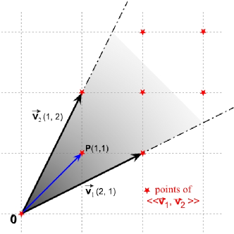
Figure 1: Example of $\mathbb{R}$-sector and $\mathcal{G}$-sector in $\left(\mathbb{Z}^{2},\mathbb{Z},+,\cdot\right)$.

Remark 2.2   It is possible that a $\mathcal{G}$-sector does not correspond to the set of points ${\mathbf{p}}$ such that ${\mathbf{p}}=\sum_{k=1}^{n}\lambda_{k}{\overrightarrow{\mathbf{v}}}_{k}\textrm{, }\lambda_{k}\in\mathcal{R}^{+}$. For example, as illustrated in Figure 1, if we take the module $\left(\mathbb{Z}^{2},\mathbb{Z},+,\cdot\right)$, the point ${\mathbf{p}}{\scriptstyle{\overrightarrow{\mathbf{(1,1)}}}}$ lies in the $\mathbb{R}$-sector $\left\langle{\overrightarrow{\mathbf{v}}}_{1}={\scriptstyle{\overrightarrow{\mathbf{(2,1)}}}},{\overrightarrow{\mathbf{v}}}_{2}={\scriptstyle{\overrightarrow{\mathbf{(1,2)}}}}\right\rangle$ $\left({\overrightarrow{\mathbf{(1,1)}}}=1/3\cdot{\overrightarrow{\mathbf{(2,1)}}}+1/3\cdot{\overrightarrow{\mathbf{(1,2)}}}\right)$ and as it is a point of $\mathbb{Z}^{2}$, it also lies in the $\mathcal{G}$-sector $\langle\langle{\overrightarrow{\mathbf{v}}}_{1},{\overrightarrow{\mathbf{v}}}_{2}\rangle\rangle$. But it cannot be written as $\lambda_{1}\cdot{\overrightarrow{\mathbf{v}}}_{1}+\lambda_{2}\cdot{\overrightarrow{\mathbf{v}}}_{2}$ with $\lambda_{1},\lambda_{2}\in\mathbb{Z}$. $\blacklozenge$

Definition 2.13 (Wedge of a chamfer mask)

We call a wedge of a chamfer mask $\mathcal{C}$, a $\mathcal{G}$-sector formed by a family $\mathcal{F}=\left({\overrightarrow{\mathbf{v}}}_{i_{k}}\right)_{k=1..n}$ of $n$ vectors of $\mathcal{C}$ which does not contain any other vector of $\mathcal{C}$.

To avoid the situation illustrated in Remark 2.2 we consider only $\mathcal{G}$-sectors based on a basis of $\mathcal{G}$.

Definition 2.14 ($\mathcal{G}$-basis-sector)

We call a $\mathcal{G}$-sector $\langle\langle{\overrightarrow{\mathbf{v}}}_{1},...{\overrightarrow{\mathbf{v}}}_{n}\rangle\rangle$ where
$\left({\overrightarrow{\mathbf{v}}}_{k}\right)_{k=1..n}$ is a basis of $\left(\mathcal{G},\mathcal{R},+,\cdot\right)$ a $\mathcal{G}$-basis-sector.

By definition of a basis, a $\mathcal{G}$-basis-sector corresponds exactly to the the set of points ${\mathbf{p}}$ such that ${\overrightarrow{\mathbf{p}}}=\sum_{k=1}^{n}\lambda_{k}{\overrightarrow{\mathbf{v}}}_{k},\lambda_{k}\in\mathcal{R}^{+}$.

Given a family $\mathcal{F}=\left({\overrightarrow{\mathbf{v}}}_{k}\right)_{k\in[1..n]}$ of $n$ independent vectors, we denote $\Delta_{\mathcal{F}}^{0}\in\mathcal{R}$

$$\Delta_{\mathcal{F}}^{0}=\det({\overrightarrow{\mathbf{v}}}_{1},{\overrightarrow{\mathbf{v}}}_{2},...,{\overrightarrow{\mathbf{v}}}_{n})=\left|\begin{array}[]{l l l l}v^{1}_{1}&v^{1}_{2}&\cdots&v^{1}_{n}\\ v^{2}_{1}&v^{2}_{2}&\cdots&v^{2}_{n}\\ \vdots&\vdots&\ddots&\vdots\\ v^{n}_{1}&v^{n}_{2}&\cdots&v^{n}_{n}\\ \end{array}\right|$$

and $\forall k\in[1..n]$, we consider the function $\Delta_{\mathcal{F}}^{k}\ \colon\ \left\{\begin{array}[]{l}\mathcal{G}\longrightarrow\mathcal{R}\\ {\overrightarrow{\mathbf{x}}}\longmapsto\Delta_{\mathcal{F}}^{k}({\overrightarrow{\mathbf{x}}})\\ \end{array}\right.$ such that:

$$\Delta_{\mathcal{F}}^{k}({\overrightarrow{\mathbf{x}}})=\det({\overrightarrow{\mathbf{v}}}_{1},...,{\overrightarrow{\mathbf{v}}}_{k-1},{\overrightarrow{\mathbf{x}}},{\overrightarrow{\mathbf{v}}}_{k+1},...,{\overrightarrow{\mathbf{v}}}_{n})=\left|\begin{array}[]{c c c c c c c}v^{1}_{1}&\cdots&v_{k-1}^{1}&x^{1}&v_{k+1}^{1}&\cdots&v_{n}^{1}\\ v^{2}_{1}&\cdots&v_{k-1}^{2}&x^{2}&v_{k+1}^{2}&\cdots&v_{n}^{2}\\ \vdots&\ddots&\vdots&\vdots&\vdots&\ddots&\vdots\\ v^{n}_{1}&\cdots&v_{k-1}^{n}&x^{n}&v_{k+1}^{n}&\cdots&v_{n}^{n}\\ \end{array}\right|.$$

Lemma 2.1

A family $\mathcal{F}=\left({\overrightarrow{\mathbf{v}}}_{k}\right)_{k\in[1..n]}$ is a basis of $\left(\mathcal{G},\mathcal{R},+,\cdot\right)$, iff

$$\forall{\overrightarrow{\mathbf{x}}}\in\mathcal{G}\textrm{, }\forall k\in[1..n]\textrm{ }\frac{1}{\Delta_{\mathcal{F}}^{0}}\times\Delta_{\mathcal{F}}^{k}({\overrightarrow{\mathbf{x}}})\in\mathcal{R}.$$

Proof.  The proof in $\left(\mathbb{Z}^{2},\mathbb{Z}\right)$ can be found in [29].
By definition of a basis, a family $\mathcal{F}=\left({\overrightarrow{\mathbf{v}}}_{k}\right)_{k\in[1..n]}$ is a basis of $\left(\mathcal{G},\mathcal{R},+,\cdot\right)$ iff $\forall{\mathbf{x}}\in\mathcal{G}$, $\exists\alpha_{1},\alpha_{2},...,\alpha_{n}\in\mathcal{R}$ such that ${\mathbf{x}}=\sum_{k=1}^{n}\alpha_{k}\cdot{\overrightarrow{\mathbf{v}}}_{k}$.
As we consider sub-modules of $\mathbb{R}^{n}$, ${\mathbf{x}}\in\mathbb{R}^{n}$ and $\forall k\in[1..n]$, ${\overrightarrow{\mathbf{v}}}_{k}\in\mathbb{R}^{n}$. If the vectors of $\mathcal{F}$ are not independent, $\mathcal{F}$ is not a basis of $\mathcal{G}$, and as $\Delta_{\mathcal{F}}^{0}=0$, $\forall{\overrightarrow{\mathbf{x}}}\in\mathcal{G},\frac{1}{\Delta_{\mathcal{F}}^{0}}\Delta_{\mathcal{F}}^{k}({\overrightarrow{\mathbf{x}}})\not\in\mathcal{R}$. If $\mathcal{F}$ is an independent family of vectors, as $\mathbb{R}^{n}$ is a vector space, $\mathcal{F}$ is a basis of $\left(\mathbb{R}^{n},\mathbb{R}\right)$ and $\exists\alpha_{1},\alpha_{2},...,\alpha_{n}\in\mathbb{R}$ such that ${\mathbf{x}}=\sum_{k=1}^{n}\alpha_{k}\cdot{\overrightarrow{\mathbf{v}}}_{k}$. This can be written:

$$\begin{array}[]{c c c}\left(\begin{array}[]{c}x^{1}\\ x^{2}\\ \vdots\\ x^{n}\end{array}\right)=&\underbrace{\left(\begin{array}[]{c c c c}v^{1}_{1}&v^{1}_{2}&\cdots&v^{1}_{n}\\ v^{2}_{1}&v^{2}_{2}&\cdots&v^{2}_{n}\\ \vdots&\vdots&\ddots&\vdots\\ v^{n}_{1}&v^{n}_{2}&\cdots&v^{n}_{n}\end{array}\right)}&\times\left(\begin{array}[]{c}\alpha_{1}\\ \alpha_{2}\\ \vdots\\ \alpha_{n}\end{array}\right)\\ &\mathcal{M}_{\mathcal{F}}&\end{array}$$

As $\mathcal{F}$ is an independent family, $\Delta_{\mathcal{F}}^{0}=\det(\mathcal{M}_{\mathcal{F}})\neq 0$ and the matrix $\mathcal{M}_{\mathcal{F}}$ can be inverted such that

$$\left(\begin{array}[]{c}\alpha_{1}\\ \alpha_{2}\\ \vdots\\ \alpha_{n}\end{array}\right)=\left(\begin{array}[]{c c c c}v^{1}_{1}&v^{1}_{2}&\cdots&v^{1}_{n}\\ v^{2}_{1}&v^{2}_{2}&\cdots&v^{2}_{n}\\ \vdots&\vdots&\ddots&\vdots\\ v^{n}_{1}&v^{n}_{2}&\cdots&v^{n}_{n}\end{array}\right)^{-1}\left(\begin{array}[]{c}x^{1}\\ x^{2}\\ \vdots\\ x^{n}\end{array}\right).$$

Inverting $\mathcal{M}_{\mathcal{F}}$ using Cramer’s rule leads to

$$\forall k\in[1..n]\textrm{, }\alpha_{k}=\frac{1}{\Delta_{\mathcal{F}}^{0}}\times\Delta_{\mathcal{F}}^{k},$$

and $\mathcal{F}$ is a basis of $\left(\mathcal{G},\mathcal{R}\right)$ iff $\forall k\in[1..n]$, $\alpha_{k}\in\mathcal{R}$. $\blacksquare$
When $\left(\mathcal{G},\mathcal{R}\right)=\left(\mathbb{Z}^{n},\mathbb{Z}\right)$ we obtain the condition $\Delta_{\mathcal{F}}^{0}=\pm 1$ for cone regularity defined in [30].

We can always organize $\mathcal{C}$ as a set of wedges (taking $n$-tuples of vectors that do not contain any other vectors). To avoid the situation in Remark 2.2 and to be able to forecast the final weighted distance from the chamfer mask, we choose masks whose wedges are all $\mathcal{G}$-basis. When $(\mathcal{G},\mathcal{R})=(\mathbb{Z}^{2},\mathbb{Z})$, taking every couple $({\overrightarrow{\mathbf{u}}},{\overrightarrow{\mathbf{v}}})$ of adjacent vectors of $\mathcal{C}$ in clockwise (or counter-clockwise) order gives such an organization. If, for each couple $\det({\overrightarrow{\mathbf{u}}},{\overrightarrow{\mathbf{v}}})=\pm 1$, then, they are a $\mathcal{G}$-basis (cf. [24]). For example, in Figure 2 of Remark 2.1, $\left\{{\scriptstyle\langle\langle{\overrightarrow{\mathbf{v}}}_{1},{\overrightarrow{\mathbf{v}}}_{2}\rangle\rangle}\right.$, ${\scriptstyle\langle\langle{\overrightarrow{\mathbf{v}}}_{2},{\overrightarrow{\mathbf{v}}}_{3}\rangle\rangle}$, ${\scriptstyle\langle\langle{\overrightarrow{\mathbf{v}}}_{3},-{\overrightarrow{\mathbf{v}}}_{1}\rangle\rangle}$, ${\scriptstyle\langle\langle-{\overrightarrow{\mathbf{v}}}_{1},-{\overrightarrow{\mathbf{v}}}_{2}\rangle\rangle}$, ${\scriptstyle\langle\langle-{\overrightarrow{\mathbf{v}}}_{2},-{\overrightarrow{\mathbf{v}}}_{3}\rangle\rangle}$, $\left.{\scriptstyle\langle\langle-{\overrightarrow{\mathbf{v}}}_{3},{\overrightarrow{\mathbf{v}}}_{1}\rangle\rangle}\right\}$ is an organization of $\mathcal{C}$ in $G$-basis wedges. For $n\geq 3$, this organization may be more complicated. Indeed several ways of organizing $n+1$ independent vectors into two wedges may exist: for example, if we take the vectors ${\overrightarrow{\mathbf{v}}}_{1}={\overrightarrow{\mathbf{(1,0,0)}}}$, ${\overrightarrow{\mathbf{v}}}_{2}={\overrightarrow{\mathbf{(1,1,0)}}}$, ${\overrightarrow{\mathbf{v}}}_{3}={\overrightarrow{\mathbf{(1,1,1)}}}$, ${\overrightarrow{\mathbf{v}}}_{4}={\overrightarrow{\mathbf{(1,0,1)}}}$ and their symmetric vectors, the wedges $\langle\langle{\overrightarrow{\mathbf{v}}}_{1},{\overrightarrow{\mathbf{v}}}_{2},{\overrightarrow{\mathbf{v}}}_{3}\rangle\rangle$ and $\langle\langle{\overrightarrow{\mathbf{v}}}_{3},{\overrightarrow{\mathbf{v}}}_{4},{\overrightarrow{\mathbf{v}}}_{1}\rangle\rangle$ are a $\mathcal{G}$-basis, but we can also consider the wedges $\langle\langle{\overrightarrow{\mathbf{v}}}_{4},{\overrightarrow{\mathbf{v}}}_{1},{\overrightarrow{\mathbf{v}}}_{2}\rangle\rangle$ and $\langle\langle{\overrightarrow{\mathbf{v}}}_{2},{\overrightarrow{\mathbf{v}}}_{3},{\overrightarrow{\mathbf{v}}}_{4}\rangle\rangle$. In [31], an automatic recursive method is given; it is based on Farey series to organize chamfer masks of $(\mathbb{Z}^{3},\mathbb{Z})$ with $\mathcal{G}$-basis wedges. In the general case, considering a mask $\mathcal{C}$ containing only a $\mathcal{G}$-basis $\mathcal{F}=({\overrightarrow{\mathbf{v}}}_{k},w_{k})_{k=1..n}$ and their symmetric wedges $\mathcal{F}_{0}=(-{\overrightarrow{\mathbf{v}}}_{k},w_{k})_{k=1..n}$, leads to two $\mathcal{G}$-basis wedges (if $\forall{\overrightarrow{\mathbf{x}}}\in\mathcal{G},\forall k\in[1..n],\frac{1}{\Delta_{\mathcal{F}}^{0}}\Delta_{\mathcal{F}}^{k}({\overrightarrow{\mathbf{x}}})\in\mathcal{R}$, $\frac{1}{\Delta_{\mathcal{F}_{0}}^{0}}\Delta_{\mathcal{F}_{0}}^{k}({\overrightarrow{\mathbf{x}}})=\pm\frac{1}{\Delta_{\mathcal{F}}^{0}}\Delta_{\mathcal{F}}^{k}({\overrightarrow{\mathbf{x}}})\in\mathcal{R}$ as $\mathcal{R}$ is a group). Moreover, the other wedges are $\mathcal{F}_{l}=({\overrightarrow{\mathbf{v}}}_{1},...,{\overrightarrow{\mathbf{v}}}_{l-1},-{\overrightarrow{\mathbf{v}}}_{l},{\overrightarrow{\mathbf{v}}}_{l+1},...,{\overrightarrow{\mathbf{v}}}_{n})$ for $l\in[1..n]$. They all are $\mathcal{G}$-basis wedges as $\forall{\overrightarrow{\mathbf{x}}}\in\mathcal{G},\forall l\in[1..n],\frac{1}{\Delta_{\mathcal{F}_{l}}^{0}}\Delta_{\mathcal{F}_{l}}^{k}(x)=\pm\frac{1}{\Delta_{\mathcal{F}}^{0}}\Delta_{\mathcal{F}}^{k}(x)\in\mathcal{R}$ as $\mathcal{R}$ is a group. We can then add vectors to this mask, taking care of keeping an organization in $\mathcal{G}$-basis wedges.

Remark 2.3   Given a chamfer mask $\mathcal{C}=\{({\overrightarrow{\mathbf{v}}}_{k},w_{k})_{k\in[1..n]}\in\mathcal{G}\times\mathcal{R}\}$ which is organized in $\mathcal{G}$-basis wedges, and given any point ${\mathbf{p}}$ lying in a wedge $\langle\langle{\overrightarrow{\mathbf{v}}}_{i_{1}},...,{\overrightarrow{\mathbf{v}}}_{i_{n}}\rangle\rangle$ of $\mathcal{C}$, there exist a path $\mathcal{P}_{{\mathbf{p}}}=\sum_{k=1}^{n}\alpha_{k}{\overrightarrow{\mathbf{v}}}_{k}$ with $\forall k\in[1..n]$ (i.e. the point ${\mathbf{p}}$ can by reached by a linear combination of only $n$ vectors among the $m$ vectors of the mask $\mathcal{C}$ with coefficients in $\mathcal{R}^{+}$). However, the final weighted distance at this point may not be a linear combination of the $n$ weights corresponding to these $n$ vectors in the chamfer mask.

For example, in $\left(\mathbb{Z}^{2},\mathbb{Z}\right)$, let us consider the mask $\mathcal{C}$ containing the weighted vectors $\left({\overrightarrow{\mathbf{v}}}_{1},w_{1}\right)=\left({\overrightarrow{\mathbf{(1,0)}}},2\right)$, $\left({\overrightarrow{\mathbf{v}}}_{2},w_{2}\right)=\left({\overrightarrow{\mathbf{(2,1)}}},5\right)$, $\left({\overrightarrow{\mathbf{v}}}_{3},w_{3}\right)=\left({\overrightarrow{\mathbf{(1,1)}}},1\right)$ and their symmetric vectors. The families $\mathcal{F}_{1}=\left({\overrightarrow{\mathbf{v}}}_{1},{\overrightarrow{\mathbf{v}}}_{2}\right)$ and $\mathcal{F}_{2}=\left({\overrightarrow{\mathbf{v}}}_{2},{\overrightarrow{\mathbf{v}}}_{3}\right)$, generating the wedges $\mathcal{S}_{1}=\langle\langle{\overrightarrow{\mathbf{v}}}_{1},{\overrightarrow{\mathbf{v}}}_{2}\rangle\rangle$ and $\mathcal{S}_{2}=\langle\langle{\overrightarrow{\mathbf{v}}}_{2},{\overrightarrow{\mathbf{v}}}_{3}\rangle\rangle$ respectively, are a basis of $(\mathbb{Z}^{2},\mathbb{Z})$. Indeed, $\Delta_{\mathcal{F}_{1}}^{0}=\left|\begin{array}[]{c c}1&2\\ 0&1\\ \end{array}\right|=1$ and $\forall{\overrightarrow{\mathbf{x}}}\in\mathbb{Z}^{2}$, $x^{1}$, $x^{2}\in\mathbb{Z}$ and:

$$\frac{1}{\Delta_{\mathcal{F}_{1}}^{0}}\times\Delta_{\mathcal{F}_{1}}^{1}({\overrightarrow{\mathbf{x}}})=\frac{1}{1}\times\left|\begin{array}[]{c c}x^{1}&2\\ x^{2}&1\\ \end{array}\right|=1\cdot x^{1}-2\cdot x^{2}\in\mathbb{Z}$$

$$\frac{1}{\Delta_{\mathcal{F}_{1}}^{0}}\times\Delta_{\mathcal{F}_{1}}^{2}({\overrightarrow{\mathbf{x}}})=\frac{1}{1}\times\left|\begin{array}[]{c c}1&x^{1}\\ 0&x^{2}\\ \end{array}\right|=1\cdot x^{2}-0\cdot x^{1}\in\mathbb{Z}.$$

In the same way for $\mathcal{F}_{2}$, we have: $\Delta_{\mathcal{F}_{2}}^{0}=\left|\begin{array}[]{c c}2&1\\ 1&1\\ \end{array}\right|=1$ and $\forall{\overrightarrow{\mathbf{x}}}\in\mathbb{Z}$, $x^{1}$, $x^{2}\in\mathbb{Z}$ and:

$$\frac{1}{\Delta_{\mathcal{F}_{2}}^{0}}\times\Delta_{\mathcal{F}_{2}}^{1}({\overrightarrow{\mathbf{x}}})=\frac{1}{1}\times\left|\begin{array}[]{c c}x^{1}&1\\ x^{2}&1\\ \end{array}\right|=1\cdot x^{1}-1\cdot x^{2}\in\mathbb{Z}$$

$$\frac{1}{\Delta_{\mathcal{F}_{2}}^{0}}\times\Delta_{\mathcal{F}_{2}}^{2}({\overrightarrow{\mathbf{x}}})=\frac{1}{1}\times\left|\begin{array}[]{c c}2&x^{1}\\ 1&x^{2}\\ \end{array}\right|=2\cdot x^{2}-1\cdot x^{1}\in\mathbb{Z}$$

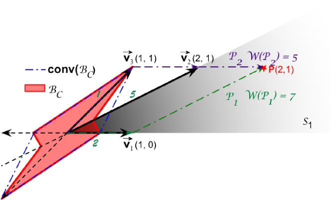
Figure 2: Example where the weighted distance does not depend on $\mathcal{G}$-basis sector vectors.

However, as illustrated in Figure 2 the point ${\mathbf{p}}=(2,1)$ lying in the $\mathcal{G}$-basis-sector $\mathcal{S}_{1}$ can be reached only by the path $\mathcal{P}_{1}=1\cdot{\overrightarrow{\mathbf{v}}}_{1}+1\cdot{\overrightarrow{\mathbf{v}}}_{2}=1\cdot{\overrightarrow{\mathbf{v}}}_{2}+1\cdot{\overrightarrow{\mathbf{v}}}_{1}$ containing only vectors of $\mathcal{F}_{1}$ and $\mathcal{W}(\mathcal{P}_{1})=w_{1}+w_{2}=2+5=7$. But ${\mathbf{p}}$ can also be reached by the following path $\mathcal{P}_{2}=2\cdot{\overrightarrow{\mathbf{v}}}_{1}+1\cdot{\overrightarrow{\mathbf{v}}}_{3}=1\cdot{\overrightarrow{\mathbf{v}}}_{3}+2\cdot{\overrightarrow{\mathbf{v}}}_{1}$ belonging neither to the sector $\mathcal{S}_{1}$ nor to the sector $\mathcal{S}_{2}$ with a cost $\mathcal{W}(\mathcal{P}_{2})=2\times w_{1}+w_{3}=2\times 2+1=5$. As the weighted distance of a point (with respect to the origin) is the minimum cost of all paths allowed by the mask, we have $d_{\mathcal{C}}({\mathbf{p}})\leq 5$ and thus $d_{\mathcal{C}}({\mathbf{p}})\neq\mathcal{W}(\mathcal{P}_{1})$. $\blacklozenge$

To avoid the situation mentioned in Remark 2.1, we add restrictions to the mask weights. These restrictions rely on the fact that the polytope formed by the chamfer mask vectors normalized by their weights is convex.

Definition 2.15 (Normalized chamfer mask polytope)

We call the polytope of $\mathbb{R}^{n}$ whose faces are the $n-1$-dimensional pyramids formed by the $n$ vectors of each wedge of a chamfer mask $\mathcal{M}_{C}=\{({\overrightarrow{\mathbf{v}}}_{k},w_{k})_{k\in[1..m]}\in\mathcal{G}\times\mathcal{R}\}$ normalized by their weights, i.e. ${\mathbf{\widetilde{v}}}_{i_{k}}=\frac{1}{w_{i_{k}}}\cdot{\mathbf{v}}_{i_{k}}\textrm{, }k\in[1..n]$ for each wedge $\langle\langle{\overrightarrow{\mathbf{v}}}_{i_{1}},...,{\overrightarrow{\mathbf{v}}}_{i_{n}}\rangle\rangle$ of $\mathcal{C}$ the normalized chamfer mask polytope, denoted $\mathcal{B}_{\mathcal{C}}$ . Note that as $(\mathcal{G},\mathcal{R},+,\cdot)$ is a module but not a vector space, these points may not be in $\mathcal{G}$.

Lemma 2.2

If the normalized polytope $\mathcal{B}_{\mathcal{C}}$ is convex, the weighted distance of any point ${\mathbf{p}}$ lying inside a wedge $\langle\langle{\overrightarrow{\mathbf{v}}}_{i_{1}},...{\overrightarrow{\mathbf{v}}}_{i_{n}}\rangle\rangle$ of a chamfer mask $\mathcal{C}=\{({\overrightarrow{\mathbf{v}}}_{k},w_{k})_{k\in[1..n]}\in\mathcal{G}\times\mathcal{R}\}$ depends only on the weights $w_{i_{1}},...,w_{i_{n}}$.

Proof.  This proof can be found in [24] for $(\mathbb{Z}^{2},\mathbb{Z})$.
If ${\mathbf{p}}={\mathbf{O}}$, the proof is obvious. Let a point ${\mathbf{p}}\neq{\mathbf{O}}$, ${\mathbf{p}}\in\langle\langle{\overrightarrow{\mathbf{v}}}_{i_{1}},...,{\overrightarrow{\mathbf{v}}}_{i_{n}}\rangle\rangle$ be given. As $\mathcal{F}=({\overrightarrow{\mathbf{v}}}_{i_{1}},...,{\overrightarrow{\mathbf{v}}}_{i_{n}})$ is a $\mathcal{G}$-basis, there exists a path $\mathcal{P}=\sum_{k=1}^{n}\alpha_{k}{\overrightarrow{\mathbf{v}}}_{i_{k}}$ from ${\mathbf{O}}$ to ${\mathbf{p}}$ containing only vectors of $\mathcal{F}$ having positive coefficients ($\forall k\in[1..n],\alpha_{k}\geq 0$). The cost of this path is $\mathcal{W}(\mathcal{P})=\sum_{k=1}^{n}\alpha_{k}\times w_{i_{k}}$. We can write $\mathcal{P}$ as

$$\mathcal{P}=\left(\sum_{l=1}^{n}\alpha_{l}\times w_{i_{l}}\right)\times\sum_{k=1}^{n}\frac{\alpha_{k}\times w_{i_{k}}}{\sum_{l=1}^{n}\alpha_{l}\times w_{i_{l}}}\times\frac{1}{w_{i_{k}}}\cdot{\overrightarrow{\mathbf{v}}}_{i_{k}}=\mathcal{W}(\mathcal{P})\cdot{\overrightarrow{\mathbf{u}}}_{\mathcal{P}}$$

with

$${\overrightarrow{\mathbf{u}}}_{\mathcal{P}}=\sum_{k=1}^{n}\frac{\alpha_{k}\times w_{i_{k}}}{\sum_{l=1}^{n}\alpha_{l}\times w_{i_{l}}}\cdot{\mathbf{\widetilde{v}}}_{i_{k}}.$$

Since ${\overrightarrow{\mathbf{u}}}_{\mathcal{P}}$ is a convex combination of the $n$ normalized vectors of $\mathcal{F}\colon\forall k\in[1..n]$, $0\leq\frac{\alpha_{k}\times w_{i_{k}}}{\sum_{k=1}^{n}\alpha_{k}\times w_{i_{k}}}\leq 1$ and $\sum_{k=1}^{n}\frac{\alpha_{k}\times w_{i_{k}}}{\sum_{k=1}^{n}\alpha_{k}\times w_{i_{k}}}=1$, ${\overrightarrow{\mathbf{u}}}_{\mathcal{P}}$ lies on $\mathcal{B}_{\mathcal{C}}$. Moreover, as the faces of $\mathcal{B}_{\mathcal{C}}$ are convex ($n-1$-dimensional polytope with $n$ vertices) ${\overrightarrow{\mathbf{u}}}_{\mathcal{P}}$ also lies on the face formed by the family $\mathcal{F}$ of $\mathcal{B}_{\mathcal{C}}$, i.e. on the boundary of $\mathcal{B}_{\mathcal{C}}$.
Let us now consider another path $\mathcal{Q}=\sum_{k=1}^{m}\beta_{k}{\overrightarrow{\mathbf{v}}}_{k}$ from ${\mathbf{O}}$ to ${\mathbf{p}}$ containing arbitrary vectors of $\mathcal{C}$. As $\mathcal{C}$ is symmetric, we can take $\forall k\in[1..n],\beta_{k}\geq 0$ without loss of generality. Then $\mathcal{W}(\mathcal{Q})\geq\mathcal{W}(\mathcal{P})$. Indeed,

$$\mathcal{Q}=\left(\sum_{k=1}^{m}\beta_{k}w_{{k}}\right)\cdot\sum_{k=1}^{m}\frac{\beta_{k}\times w_{k}}{\sum_{k=1}^{m}\beta_{k}\times w_{k}}\times\frac{1}{w_{k}}\cdot{\overrightarrow{\mathbf{v}}}_{k}=\mathcal{W}(\mathcal{Q})\cdot{\overrightarrow{\mathbf{u}}}_{\mathcal{Q}}$$

with

$${\overrightarrow{\mathbf{u}}}_{\mathcal{Q}}=\sum_{k=1}^{m}\frac{\beta_{k}\times w_{k}}{\sum_{k=1}^{m}\beta_{k}\times w_{k}}\cdot{\mathbf{\widetilde{v}}}_{k}.$$

${\overrightarrow{\mathbf{u}}}_{\mathcal{Q}}$ is a convex combination of $m$ normalized vectors of $\mathcal{C}$, and lies thus within the convex polytope $\mathcal{B}_{\mathcal{C}}$. Moreover, we have ${\overrightarrow{\mathbf{Op}}}=\mathcal{P}=\mathcal{W}(\mathcal{P})\cdot{\overrightarrow{\mathbf{u}}}_{\mathcal{P}}=\mathcal{W}(\mathcal{Q})\cdot{\overrightarrow{\mathbf{u}}}_{\mathcal{Q}}=\mathcal{Q}$ with ${\overrightarrow{\mathbf{u}}}_{\mathcal{P}}$ and ${\overrightarrow{\mathbf{u}}}_{\mathcal{Q}}$ having the same direction (${\overrightarrow{\mathbf{Op}}}$) with positive coefficients. $\mathcal{W}_{\mathcal{P}}\left\|{\overrightarrow{\mathbf{u}}}_{\mathcal{P}}\right\|=\mathcal{W}_{\mathcal{Q}}\left\|{\overrightarrow{\mathbf{u}}}_{\mathcal{Q}}\right\|$. As ${\overrightarrow{\mathbf{u}}}_{\mathcal{Q}}$ lies within $\mathcal{B}_{\mathcal{C}}$ and ${\overrightarrow{\mathbf{u}}}_{\mathcal{P}}$ lies on the boundary of $\mathcal{B}_{\mathcal{C}}$, $\left\|{\overrightarrow{\mathbf{u}}}_{\mathcal{P}}\right\|\geq\left\|{\overrightarrow{\mathbf{u}}}_{\mathcal{Q}}\right\|$ (as $\mathcal{B}_{\mathcal{C}}$ is centered in ${\mathbf{O}}$, if $\left\|{\overrightarrow{\mathbf{u}}}_{\mathcal{Q}}\right\|>\left\|{\overrightarrow{\mathbf{u}}}_{\mathcal{P}}\right\|$, ${\mathbf{u}}_{\mathcal{Q}}$ would be farther from the origin than a point of the boundary, and thus outside $\mathcal{B}_{\mathcal{C}}$) thus $\mathcal{W}(\mathcal{P})\leq\mathcal{W}(\mathcal{Q})$ and $d_{\mathcal{C}}({\mathbf{p}})=\mathcal{W}(\mathcal{P})$. $\blacksquare$
Figure 3 shows an example of vectors ${\overrightarrow{\mathbf{u}}}_{\mathcal{P}}$ and ${\overrightarrow{\mathbf{u}}}_{\mathcal{Q}}$ of a mask $\mathcal{C}\in\left(\mathbb{Z}^{2},\mathbb{Z}\right)$.

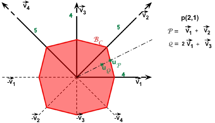
Figure 3: Example where $\mathcal{B}_{\mathcal{C}}$ is convex. We consider the vectors ${\mathbf{v}}_{1}(1,0)\textrm{, }{\mathbf{v}}_{2}(1,1)\textrm{, }{\mathbf{v}}_{3}(0,1)\textrm{, }{\mathbf{v}}_{4}(-1,1)$ and the mask $\mathcal{C}=\left\{({\mathbf{v}}_{1},4)\right.$, $({\mathbf{v}}_{2},5)$, $({\mathbf{v}}_{3},4)$, $(-{\mathbf{v}}_{1},4)$, $(-{\mathbf{v}}_{2},5)$, $\left.(-{\mathbf{v}}_{3},4)\right\}$. We consider the path $\mathcal{P}={\mathbf{v}}_{1}+{\mathbf{v}}_{2}$ and $\mathcal{Q}=2\cdot{\mathbf{v}}_{1}+{\mathbf{v}}_{3}$ from ${\mathbf{O}}$ to ${\mathbf{p}}(2,1)$. We then have $\|{\mathbf{u}}_{\mathcal{Q}}\|\leq\|{\mathbf{u}}_{\mathcal{P}}\|$.

Corollary 2.2

If the vertices of each face of the convex hull $\textrm{{conv}}(\mathcal{B}_{\mathcal{C}})$ of $\mathcal{B}_{\mathcal{C}}$ are normalized vectors corresponding to $\mathcal{G}$-basis sectors of $\mathcal{C}$, then the vectors of $\mathcal{C}$ whose corresponding normalized vectors do not lie on the convex hull of $\mathcal{B}_{\mathcal{C}}$ are not used to compute the final weighted distance.

Proof.  The proof can be found in [32, 28] for vectorial spaces. Suppose there exists a vector ${\overrightarrow{\mathbf{v}}}_{l}\in\mathcal{C}$ such that ${\overrightarrow{\mathbf{\widetilde{v}}}}_{l}=\frac{1}{w_{l}}{\overrightarrow{\mathbf{v}}}_{l}$ does not lie on the convex hull of $\mathcal{B}_{\mathcal{C}}$ (i.e. ${\overrightarrow{\mathbf{\widetilde{v}}}}_{l}$ lies within $\mathcal{B}_{\mathcal{C}}$). Let us consider the $\mathcal{G}$-basis sector $\langle\langle{\overrightarrow{\mathbf{v}}}_{i_{1}},...,{\overrightarrow{\mathbf{v}}}_{i_{n}}\rangle\rangle$ in which ${\overrightarrow{\mathbf{v}}}_{l}$ lies and whose corresponding normalized vectors form a face $\mathcal{F}$ of $\textrm{conv}(\mathcal{B}_{\mathcal{C}})$. There exists a path $\mathcal{P}=\sum_{k=1}^{n}\alpha_{k}{\overrightarrow{\mathbf{v}}}_{i_{k}}={\overrightarrow{\mathbf{v}}}_{l}$ from ${\mathbf{O}}$ to ${\mathbf{v}}_{l}$ and with $\mathcal{W}(\mathcal{P})<w_{l}$. Indeed, ${\overrightarrow{\mathbf{v}}}_{l}=w_{l}{\overrightarrow{\mathbf{\widetilde{v}}}}_{l}=\mathcal{W}(\mathcal{P}){\overrightarrow{\mathbf{u}}}_{\mathcal{P}}$ with ${\overrightarrow{\mathbf{u}}}_{\mathcal{P}}=\sum_{k=1}^{n}\frac{\alpha_{k}w_{i_{k}}}{\sum_{k=1}^{n}\alpha_{k}w_{i_{k}}}{\overrightarrow{\mathbf{\widetilde{v}}}}_{i_{k}}$ a convex combination of $n$ vectors of $\mathcal{F}$ lying within $\mathcal{F}$. We thus have $\left\|{\overrightarrow{\mathbf{\widetilde{v}}}}_{l}\right\|<\left\|{\overrightarrow{\mathbf{u}}}_{\mathcal{P}}\right\|$ and $w_{l}>\mathcal{W}(\mathcal{P})$. Finally, as a weighted distance is the minimum of the costs of all possible path, in any path containing ${\overrightarrow{\mathbf{v}}}_{l}$, ${\overrightarrow{\mathbf{v}}}_{l}$ will be replaced by $\mathcal{P}$ whose cost is lower. Note that this is what happens in Remark 2.1. $\blacksquare$

Remark 2.4   If there exist faces of $\textrm{conv}(\mathcal{B}_{\mathcal{C}})$ formed by normalized vectors whose corresponding mask vectors are not $\mathcal{G}$-basis, the vectors of $\mathcal{C}$ which does not lie on $\textrm{conv}(\mathcal{B}_{\mathcal{C}})$ may be used, but this leads to a final weighted distance which may not be homogeneous along some directions, and we also may not be able to forecast the weighted distance inside a wedge with the only vectors generating the wedge.

For example, if we consider the mask $\mathcal{C}$ with the weighted vectors: ${\overrightarrow{\mathbf{v}}}_{1}=({\scriptstyle{\overrightarrow{\mathbf{(1,0)}}}},3)$, ${\overrightarrow{\mathbf{v}}}_{2}=({\scriptstyle{\overrightarrow{\mathbf{(1,1)}}}},2)$, ${\overrightarrow{\mathbf{v}}}_{3}=({\scriptstyle{\overrightarrow{\mathbf{(0,1)}}}},3)$, ${\overrightarrow{\mathbf{v}}}_{4}=({\scriptstyle{\overrightarrow{\mathbf{(-1,1)}}}},2)$ and their symmetric vectors, as shown in Figure 4, $d_{\mathcal{C}}({\mathbf{O}},{\mathbf{(0,2)}})=4\neq 2\times d_{\mathcal{C}}({\mathbf{O}},{\mathbf{(0,1)}})=2\times 3$. Moreover, $d_{\mathcal{C}}({\mathbf{O}},{\mathbf{(0,2)}})$ does not only depend on ${\overrightarrow{\mathbf{v}}}_{2}$ and ${\overrightarrow{\mathbf{v}}}_{3}$ or only on ${\overrightarrow{\mathbf{v}}}_{3}$ and ${\overrightarrow{\mathbf{v}}}_{4}$. Note that the vectors ${\overrightarrow{\mathbf{v}}}_{2}$ and ${\overrightarrow{\mathbf{v}}}_{4}$ generating the corresponding face of $\textrm{conv}(\mathcal{B}_{\mathcal{C}})$ do not form a $\mathbb{Z}^{2}$ basis ($\det({\overrightarrow{\mathbf{v}}}_{1},{\overrightarrow{\mathbf{v}}}_{2})=2\neq\pm 1$). $\blacklozenge$

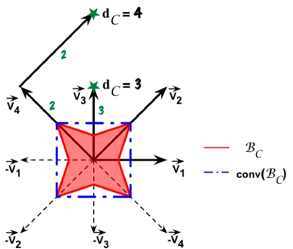
Figure 4: When $\textrm{conv}(\mathcal{B}_{\mathcal{C}})\neq\mathcal{B}_{\mathcal{C}}$ the weighted distance may not be homogeneous.

In the following, we consider only chamfer masks whose normalized polytope is convex. Indeed, if this is not the case, the mask may be redundant (Corollary 2.2), or even if not, we may not be able to forecast the final weighted distance, (Remark 2.2). We can note that this condition implies that collinear vectors (which are note opposite vectors) are removed from the mask.

Considering previous lemmas and remarks, we can re-define a chamfer mask with stronger conditions as follows:

Definition 2.16 (Chamfer mask (restricted))

A Chamfer Mask $\mathcal{C}_{\rho}$ is a finite set of weighted vectors $\{({\overrightarrow{\mathbf{v}}}_{k},w_{k})_{k\in[1..m]}\in\mathcal{G}\times\mathcal{R}\}$ which satisfies the following properties:

$$(\textrm{positive weights}) \forall k\textrm{, } w_{k}>0\textrm{ and }{\overrightarrow{\mathbf{v}}}_{k}\neq 0$$ (1)

$$(\textrm{symmetry}) ({\overrightarrow{\mathbf{v}}},w)\in\mathcal{C}_{\rho} \Longrightarrow(-{\overrightarrow{\mathbf{v}}},w)\in\mathcal{C}_{\rho}$$ (2)

$$(\textrm{Organized in }\mathcal{G}\textrm{-basis wedges}) \left.\begin{array}[]{c}\forall{\mathbf{p}}\in\mathcal{G}\\ {\scriptstyle\exists\langle\langle{\overrightarrow{\mathbf{v}}}_{i_{1}},...,{\overrightarrow{\mathbf{v}}}_{i_{n}}\rangle\rangle\in\mathcal{C}_{\rho}}\end{array}\right\} {\mathbf{p}}=\sum_{k=1}^{n}\alpha_{k}{\overrightarrow{\mathbf{v}}}_{i_{k}}$$ (5)

$$(\textrm{Convex normalized polytope}) \mathcal{B}_{\mathcal{C}_{\rho}}=\textrm{{conv}}(\mathcal{B}_{\mathcal{C}_{\rho}})$$ (6)

Theorem 2.2

Given a chamfer mask $\mathcal{C}_{\rho}=\left\{({\overrightarrow{\mathbf{v}}}_{k},w_{k})_{k\in[1..n]}\in\mathcal{G}\times\mathcal{R}\right\}$, defined as in Definition 2.16, the weighted distance of any point ${\mathbf{p}}$ lying in a wedge $\langle\langle{\overrightarrow{\mathbf{v}}}_{i_{1}},...{\overrightarrow{\mathbf{v}}}_{i_{n}}\rangle\rangle$ can be expressed by:

$$d_{\mathcal{C}_{\rho}}({\mathbf{p}})=\frac{1}{\Delta_{\mathcal{F}}^{0}}\times\sum_{k=1}^{n}\Delta_{\mathcal{F}}^{k}({\mathbf{p}})\times w_{i_{k}}$$ (7)

Proof.  This formula was given for $(\mathbb{Z}^{3},\mathbb{Z})$ in [31] without the entire proof. Let ${\mathbf{p}}$ be a point of $\mathcal{G}$ lying in the wedge $W=\langle\langle{\overrightarrow{\mathbf{v}}}_{i_{1}},...{\overrightarrow{\mathbf{v}}}_{i_{n}}\rangle\rangle$ of $\mathcal{C}_{\rho}$. As $W$ is a basis of $(\mathcal{G},\mathcal{R})$ (condition 5 of Definition 2.16) there exists a path $\mathcal{P}$ from ${\mathbf{O}}$ to ${\mathbf{p}}$ and $\alpha_{1},...,\alpha_{k}\in\mathcal{R}^{+}$ such that $\mathcal{P}={\overrightarrow{\mathbf{Op}}}=\sum_{k=1}^{m}\alpha_{k}{\overrightarrow{\mathbf{v}}}_{i_{k}}$. The proof of Lemma 2.1 gives $\forall k\in[1..n],\alpha_{k}=\frac{1}{\Delta_{\mathcal{F}}^{0}}\times\Delta_{\mathcal{F}}^{k}({\mathbf{p}})$ and the proof of Lemma 2.2 gives that the weight of $\mathcal{P}$ is minimal. Thus $d_{\mathcal{C}_{\rho}}({\mathbf{p}})=\mathcal{W}(\mathcal{P})=\frac{1}{\Delta_{\mathcal{F}}^{0}}\times\sum_{k=1}^{n}\Delta_{\mathcal{F}}^{k}({\mathbf{p}})\times w_{i_{k}}$. $\blacksquare$

Theorem 2.3

A weighted distance computed with a chamfer mask
$\mathcal{C}_{\rho}=\{({\overrightarrow{\mathbf{v}}}_{k},w_{k})_{k\in[1..m]}\in\mathcal{G}\times\mathcal{R}\}$ as defined in Definition 2.16 is a norm on $(\mathcal{G},\mathcal{R})$.

Proof.  Here, we have to show that $d_{\mathcal{C}_{\rho}}$ is definite, positive and symmetric and satisfies the triangular inequality and the positive homogeneity properties. By definition of a weighted distance (Definition 2.10), given any points ${\mathbf{p}}\in\mathcal{G}$, there exist $\alpha_{1}$, $\alpha_{2}$, …, $\alpha_{m}$ $\in\mathcal{R}$ such that $d_{\mathcal{C}_{\rho}}({\mathbf{O}},{\mathbf{p}})=d_{\mathcal{C}_{\rho}}({\mathbf{p}})=\sum_{k=1}^{n}\alpha_{k}w_{k}$ and $\mathcal{P}_{{\mathbf{p}}}={\overrightarrow{\mathbf{Op}}}={\mathbf{p}}=\sum_{k=1}^{m}\alpha_{k}{\overrightarrow{\mathbf{v}}}_{k}$ (cf. Definitions 2.8, 2.9 and 2.10).

1. Positivity (Needs conditions 1 and 2 of Definition 2.16)
   By condition 2 of Definition 2.16 we can choose $\alpha_{k}\geq 0$ for all $k\in[1..n]$. By Condition 1 we also have $w_{k}\geq 0$ for all $k\in[1..n]$. We thus have $d_{\mathcal{C}_{\rho}}({\mathbf{p}})\geq 0$.

2. Definitivity (Needs conditions 1 and 2 of Definition 2.16)
   If ${\mathbf{p}}={\mathbf{O}}$, then the path $\mathcal{P}=\sum_{k=0}^{m}0\cdot{\overrightarrow{\mathbf{v}}}_{k}$ is a path from ${\mathbf{O}}$ to ${\mathbf{p}}$ and its cost is $\mathcal{W}(\mathcal{P})=\sum_{k=0}^{m}0\times w_{k}=0$. Thus, $d_{\mathcal{C}_{\rho}}({\mathbf{p}})=\min(\mathcal{W}({\overrightarrow{\mathbf{p}}}))\leq 0$. By positivity, we also have $d_{\mathcal{C}_{\rho}}({\mathbf{p}})\geq 0$. It follows that $d_{\mathcal{C}_{\rho}}({\mathbf{p}})=0$.
   Conversely, if $d_{\mathcal{C}_{\rho}}({\mathbf{p}})=0$, as $\forall k\in[1..m]$, $w_{k}>0$, we have $\forall k\in[1..m]$, $\alpha_{k}=0$ and ${\overrightarrow{\mathbf{p}}}=\sum_{k=1}^{m}0\cdot{\overrightarrow{\mathbf{v}}}_{k}={\overrightarrow{\mathbf{0}}}$. Thus ${\mathbf{p}}={\mathbf{O}}$.

3. Symmetry (Needs the condition 2 of Definition 2.16)
   By condition 2 of Definition 2.16, we have that

   $$\mathcal{P}_{{\overrightarrow{\mathbf{pO}}}}=\sum_{k=1}^{m}\alpha_{k}(-{\overrightarrow{\mathbf{v}}}_{k})$$ (8)

   is a path from ${\mathbf{p}}$ to ${\mathbf{O}}$ and $\mathcal{W}(\mathcal{P}_{{\overrightarrow{\mathbf{pO}}}})=\mathcal{W}(\mathcal{P}_{{\overrightarrow{\mathbf{Op}}}})$. Moreover, this cost is minimal. Indeed, let us consider a path $\mathcal{Q}_{{\overrightarrow{\mathbf{pO}}}}=\sum_{k=1}^{m}\beta_{k}{\overrightarrow{\mathbf{v}}}_{k}$ such that $\mathcal{W}(\mathcal{Q}_{{\overrightarrow{\mathbf{pO}}}})<\mathcal{W}(\mathcal{P}_{{\overrightarrow{\mathbf{pO}}}})$. Then $\mathcal{Q}_{{\overrightarrow{\mathbf{Op}}}}=\sum_{k=1}^{m}\beta_{k}\cdot(-{\overrightarrow{\mathbf{v}}}_{k})$ is a path from ${\mathbf{O}}$ to ${\mathbf{p}}$ and $\mathcal{W}(\mathcal{Q}_{{\overrightarrow{\mathbf{Op}}}})<\mathcal{W}(\mathcal{P}_{{\overrightarrow{\mathbf{Op}}}})=d_{\mathcal{C}_{\rho}}({\mathbf{p}})$ which is impossible by definition of a weighted distance (Definition 2.10). Thus $d_{\mathcal{C}_{\rho}}({\mathbf{p}},{\mathbf{O}})=\mathcal{W}(\mathcal{P}_{{\overrightarrow{\mathbf{pO}}}})=d_{\mathcal{C}_{\rho}}({\mathbf{p}})$.

4. Triangular inequality (Needs conditions 1 and 2 of Definition 2.16)
   The proof can be found in [33] for $(\mathbb{Z}^{2},\mathbb{Z},+,\cdot)$ and in [34] (Corollary 3.4) for a general module. We want $\forall{\mathbf{p}},{\mathbf{q}}\in\mathcal{G}$, $d_{\mathcal{C}_{\rho}}({\mathbf{p}},{\mathbf{q}})\leq d_{\mathcal{C}_{\rho}}({\mathbf{p}})+d_{\mathcal{C}_{\rho}}({\mathbf{q}})$. Let $\mathcal{P}_{{\mathbf{q}}}=\sum_{k=1}^{m}\beta_{k}\cdot{\overrightarrow{\mathbf{v}}}_{k}$ be the minimum cost path between ${\mathbf{O}}$ and ${\mathbf{q}}$ (i.e. $d_{\mathcal{C}_{\rho}}({\mathbf{q}})=\sum_{k=1}^{m}\beta_{k}w_{k}$), and by Eq. (8), $\mathcal{P}_{-{\mathbf{p}}}=\sum_{k=1}^{m}\alpha_{k}(-{\overrightarrow{\mathbf{v}}}_{k})$. As the mask is symmetric, $\mathcal{P}_{-{\mathbf{p}}}$ can be written $\mathcal{P}_{-{\mathbf{p}}}=\sum_{k=1}^{m}\gamma_{k}{\overrightarrow{\mathbf{v}}}_{k}$ for some $\gamma_{k}$ and $\mathcal{W}(\mathcal{P}_{-{\mathbf{p}}})=\mathcal{W}(\mathcal{P}_{{\mathbf{p}}})$. Let us suppose $d_{\mathcal{C}_{\rho}}(p,q)>d_{\mathcal{C}_{\rho}}(p)+d_{\mathcal{C}_{\rho}}(q)$. The path $\mathcal{P}_{{\mathbf{pq}}}=\mathcal{P}_{-{\mathbf{p}}}+\mathcal{P}_{{\mathbf{q}}}=\sum_{k=1}^{m}(\gamma_{k}+\beta_{k}){\overrightarrow{\mathbf{v}}}_{k}={\overrightarrow{\mathbf{pO}}}+{\overrightarrow{\mathbf{Oq}}}={\overrightarrow{\mathbf{pq}}}$ is a path from ${\mathbf{p}}$ to ${\mathbf{q}}$. As $(\mathcal{R},+)$ is an Abelian group, $\mathcal{W}(\mathcal{P}_{{\overrightarrow{\mathbf{pq}}}})=\mathcal{W}(\mathcal{P}_{-{\mathbf{p}}})+\mathcal{W}(\mathcal{P}_{{\mathbf{q}}})=d_{\mathcal{C}_{\rho}}({\mathbf{p}})+d_{\mathcal{C}_{\rho}}({\mathbf{q}})<d_{\mathcal{C}_{\rho}}({\mathbf{p}},{\mathbf{q}})$ which is impossible by definition of a weighted distance (Definition 2.10). By contradiction, we have $d_{\mathcal{C}_{\rho}}({\mathbf{p}},{\mathbf{q}})\leq d_{\mathcal{C}_{\rho}}({\mathbf{p}})+d_{\mathcal{C}_{\rho}}({\mathbf{q}})$.
   Remark 2.5   Note that a decomposition in $\mathcal{G}$-basis wedges is not needed for this condition. The only condition needed is to be able to extract a basis among all mask vectors. This is the case, for example, for masks containing only vectors corresponding to knight displacements. Indeed, each wedge of this mask is not a $\mathbb{Z}$-basis (see Figure 1 and Remark 2.2. However, this mask induces a metric, [35]. $\blacklozenge$
   Remark 2.6   The triangular inequality does not depend on the choice of the weights. $\blacklozenge$
   

5. Positive homogeneity (Needs conditions 1, 2, 5 and 6 of Definition 2.16)
   The proof can be found in [30] for $(\mathbb{Z}^{3},\mathbb{Z},+,\cdot)$ and in [28] for a general module. Let be $\lambda\in\mathcal{R}$. Let $W=\langle\langle{\overrightarrow{\mathbf{v}}}_{i_{1}},...,{\overrightarrow{\mathbf{v}}}_{i_{n}}\rangle\rangle$ be the wedges of $\mathcal{C}_{\rho}$ in which ${\mathbf{p}}$ lies. By Theorem 2.2, we have $d_{\mathcal{C}_{\rho}}({\mathbf{p}})=\frac{1}{\Delta_{\mathcal{F}}^{0}}\times\sum_{k=1}^{n}\Delta_{\mathcal{F}}^{k}({\mathbf{p}})\times w_{i_{k}}$.

   If $\lambda\geq 0$, the point $\lambda\cdot{\mathbf{p}}$ also lies in the wedge $W$ (it is a point of $\mathcal{G}$, and $\lambda{\mathbf{p}}=\sum_{k=1}^{n}\lambda\times\alpha_{k}{\overrightarrow{\mathbf{v}}}_{i_{k}}$ with $\forall k\in[1..n],\lambda\times\alpha_{i_{k}}\in\mathcal{R}^{+}$). By Theorem 2.2 we have:

   $$d_{\mathcal{C}_{\rho}}(\lambda\cdot{\mathbf{p}}) = \frac{1}{\Delta_{\mathcal{F}}^{0}}\times\sum_{k=1}^{n}\Delta_{\mathcal{F}}^{k}(\lambda\cdot{\mathbf{p}})\times w_{i_{k}}$$

   $$= \frac{1}{\Delta_{\mathcal{F}}^{0}}\times\sum_{k=1}^{n}\det\left({\overrightarrow{\mathbf{v}}}_{i_{1}},...{\overrightarrow{\mathbf{v}}}_{i_{k-1}},\lambda\cdot{\overrightarrow{\mathbf{p}}},{\overrightarrow{\mathbf{v}}}_{i_{k+1}},...{\overrightarrow{\mathbf{v}}}_{i_{n}}\right)\times w_{i_{k}}$$

   $$= \frac{1}{\Delta_{\mathcal{F}}^{0}}\times\sum_{k=1}^{n}\lambda\times\det\left({\overrightarrow{\mathbf{v}}}_{i_{1}},...{\overrightarrow{\mathbf{v}}}_{i_{k-1}},{\overrightarrow{\mathbf{p}}},{\overrightarrow{\mathbf{v}}}_{i_{k+1}},...{\overrightarrow{\mathbf{v}}}_{i_{n}}\right)\times w_{i_{k}}$$

   $$= \lambda\times\frac{1}{\Delta_{\mathcal{F}}^{0}}\times\sum_{k=1}^{n}\Delta_{\mathcal{F}}^{k}({\mathbf{p}})\times w_{i_{k}}$$

   $$= \lambda\times d_{\mathcal{C}_{\rho}}({\mathbf{p}})$$

   If $\lambda<0$, $d_{\mathcal{C}_{\rho}}(\lambda\cdot{\mathbf{p}})=d_{\mathcal{C}_{\rho}}(-\lambda\cdot{\mathbf{p}})$ with $-\lambda>0$ (symmetry property) and thus, $d_{\mathcal{C}_{\rho}}(\lambda\cdot{\mathbf{p}})=-\lambda\times d_{\mathcal{C}_{\rho}}(p)=|\lambda|\times d_{\mathcal{C}_{\rho}}({\mathbf{p}})$. $\blacksquare$

$\blacksquare$

2.4 Weight optimization

In addition to their metric and norm properties, weighted distances can be made more invariant to rotation. As a weighted distance is obtained by computing the smallest weight of several paths between two points, the first improvement to obtain a weighted distance with high rotational invariance is to allow a larger number of allowed directions for the paths. This means increasing precision by increasing the number of weighted vectors of the chamfer mask.

To increase accuracy, another way is to choose suitable weights for mask vectors. This more challenging issue as been often addressed in the literature. The first optimal chamfer weights computation was performed for a 2-D $3\times 3$ mask in a square grid [25]. Then authors computed optimal weights with different optimality criteria [36, 31], for larger masks [37, 36, 38] and for anisotropic grid [39, 40, 41]. Authors of [41, 31, 42] proposed an automatic computation of optimal chamfer weights for rectangular grids.

Observe that computing the distance transform and finding optimal weights is not directly related to the problem of estimating the length of straight lines in a discrete image [43]. For optimal weights for such estimations, see [44].

In all of the previous papers, the computation of optimal chamfer weights is performed the same way:

1. First, a chamfer mask is built and decomposed in wedges.

2. Then, the final weighted distance from the origin to an arbitrary point of the grid is expressed. The variables corresponding to the mask weights are unknown, but variables corresponding to vector coordinates are known. In the general case, given a chamfer mask defined as Definition 2.16, and a point ${\mathbf{p}}\in\mathcal{G}$ lying in the wedge $\mathcal{F}=\langle\langle{\overrightarrow{\mathbf{v}}}_{i_{1}},{\overrightarrow{\mathbf{v}}}_{i_{2}},...{\overrightarrow{\mathbf{v}}}_{i_{n}}\rangle\rangle$ the value of the weighted distance at this point is

   $$d_{\mathcal{C}_{\rho}}({\mathbf{p}})=\frac{1}{\Delta_{\mathcal{F}}^{0}}\times\sum_{k=1}^{n}\Delta_{\mathcal{F}}^{k}({\mathbf{p}})\times w_{i_{k}}$$

3. In the same way, the Euclidean distance from the origin to this point ${\mathbf{p}}$ is expressed. In the general case, given a grid which is a sub-module of $\mathbb{R}^{n}$ with an elongation of $s_{1},s_{2},...,s_{n}$ in each canonical direction, the Euclidean distance between the origin and the point ${\mathbf{p}}$ can be expressed in the following way:

   $$d_{E}({\mathbf{p}})=\sqrt{\sum_{i=1}^{n}(s_{i}p^{i})^{2}}$$

4. After these three steps, the error between the weighed distance and the Euclidean one can be expressed for any point ${\mathbf{p}}\in\mathcal{G}$. This error can be either absolute (the difference between these two values) [37] or relative (the difference is divided by the Euclidean distance) [36]. The error can be expressed as follows:

   $$E({\mathbf{p}}) = d_{\mathcal{C}_{\rho}}({\mathbf{p}})-d_{E}({\mathbf{p}})$$

   $$= \frac{1}{\Delta_{\mathcal{F}}^{0}}\times\left(\sum_{k=1}^{n}\Delta_{\mathcal{F}}^{k}({\mathbf{p}})\times w_{i_{k}}\right)-\sqrt{\sum_{i=1}^{n}(s_{i}p^{i})^{2}}$$

   The general relative error can be expressed as follows:

   $$E_{rel}({\mathbf{p}}) = \frac{d_{\mathcal{C}_{\rho}}({\mathbf{p}})-d_{E}({\mathbf{p}})}{d_{E}({\mathbf{p}})}$$

   $$= \frac{\sum_{k=1}^{n}\Delta_{\mathcal{F}}^{k}({\mathbf{p}})\times w_{i_{k}}}{{\Delta_{\mathcal{F}}^{0}}\times\sqrt{\sum_{i=1}^{n}(s_{i}p^{i})^{2}}}-1$$

5. The previous errors are $n$-dimensional functions of the coordinates $p^{1},p^{2}$, … $p^{n}$ of ${\mathbf{p}}$. To reduce the number of these variables and be able to find extrema, the maximal error is computed either on a hyperplane or on a sphere. For example, in three dimensions, the error can be computed on a plane $X=T,Y=T\textrm{ or }Z=T$ [37, 31] or on the sphere of radius $T$ [42]. This error function is continuous on a compact set (the $n-1$ pyramid formed by the $n$ vectors of each wedge). Thus it is bounded and attains its bounds. These bounds can be located either at the vertices of the pyramid or inside (including other bounds such as edges) the pyramid.

6. Computing the derivatives of the error function gives the point ${\mathbf{p_{max}}}$ at which the error is maximum (due to the sign of the derivatives) inside the wedge. In this way, the maximum error within the wedge $E_{max}=E({\mathbf{p_{max}}})$ can be obtained (if ${\mathbf{p_{max}}}$ lies within the wedge).

7. The other extrema (minima) $E_{1},E_{2},...,E_{n}$ are obtained for the $n$ vectors delimiting the wedge (the vertices of the $n-1$ pyramid). When computing the error on a sphere of radius $R$, in the general case, the extrema can be expressed in the following way ($\forall l\in[1..n]$):

   $$E^{l}=\left(w_{l}-||{\overrightarrow{\mathbf{v}}}_{l}||\right)\textrm{ and }E_{rel}^{l}=\left(\frac{w_{l}}{||{\overrightarrow{\mathbf{v}}}_{l}||}-1\right)$$

   with $||{\overrightarrow{\mathbf{v}}}_{l}||=\sqrt{\sum_{k=1}^{n}(s_{k}v_{l}^{k})^{2}}$ being the Euclidean norm of the vector ${\overrightarrow{\mathbf{v}}}_{l}$ expressed in the world coordinate.

8. Minimizing the maximum error leads to computing optimal real weights with the following equation: $E_{max}=-E_{1}=-E_{2}=...=-E_{n}$.

9. A depth-first search in an integer weights tree taking the error into account can lead to optimal integer weights set for a given mask [31, 42].

We have generalized weighted distance properties found in the literature to modules. These properties are true for the well-known cubic grid, but can also be applied to other grids such as the FCC and BCC grids as we will see in Section 4. In applications, an efficient algorithm for computing distance transforms is is needed. In the following section, we discuss such an algorithm: the two-scan chamfer algorithm. We prove that the algorithm produces correct result for images on general point lattices.

3 How to compute distance maps using the chamfer algorithm

There are basically three families of algorithms for computing weighted distance transforms – bucket-sort (also known as wave-front propagation), parallel, and sequential algorithms. Initially in the bucket-sort algorithm [45], the border points of the object are stored in a list. These points are updated with the distance to the background. The distances are propagated by removing the updated points from the list and adding the neighbors of these points to the list. This is iterated until the list is empty. The parallel algorithm [46] is the most intuitive one. Given the original image, a new image is obtained by applying the chamfer mask simultaneously to each point of the image giving the minimum distance value at each of these points. This process is applied to the new image. By applying the procedure iteratively until stability, the distance map is obtained (a proof using infimal convolution is found in [34]).

Rosenfeld & Pfaltz [12] showed that this is equivalent to two sequential scans of the image for grids in $\mathbb{Z}^{2}$ and a $3\times 3$ mask. Sequential means that we use previously updated values of the same image to obtain new updated values. Two advantages are that a two-scan algorithm is enough to construct a distance map in any dimension and that the complexity is known ($O(M)$, where $M$ is the number of points in the image). The worst case complexity of the parallel algorithm is $O(M^{2})$ – $M$ iterations of operations on $M$ points. This result is now generalized and proved to be correct on any grid for which all grid point coordinates can be expressed by a basis.

In this section, $\mathcal{S}$ is a finite subset of $\mathcal{G}$ and $\mathcal{R}=\mathbb{Z}$. The cardinality of $\mathcal{S}$ is denoted $M=\textnormal{card}(\mathcal{S})$. Observe that the chamfer weights are in $\mathcal{R}^{+}=\mathbb{N}$ (Definition 2.16, condition 1) and that the weighted distance have values in $\mathcal{R}^{+}$ (Definition 2.10).

Definition 3.1

Given ${\mathbf{a}}=(a_{1},a_{2},\dots,a_{n})$, where $a_{1},a_{2},\dots,a_{n}\in\mathcal{R}$ and $\sigma\in\mathbb{R}$. Let

$$\mathcal{T}^{\mathbf{a}}_{\sigma,\square}=\left\{{\mathbf{p}}\in\mathcal{G}:a_{1}p^{1}+a_{2}p^{2}+\dots+a_{n}p^{n}\square\sigma\right\},$$

where $\square$ is one of the relations $<,\leq,=,\geq,$ or $>$.

For example, $\mathcal{T}^{\mathbf{a}}_{\sigma,=}$ is a hyperplane and $\mathcal{T}^{\mathbf{a}}_{\sigma,<}$, $\mathcal{T}^{\mathbf{a}}_{\sigma,\leq}$, $\mathcal{T}^{\mathbf{a}}_{\sigma,>}$, and $\mathcal{T}^{\mathbf{a}}_{\sigma,\geq}$ are half-spaces separated by the hyperplane $\mathcal{T}^{\mathbf{a}}_{\sigma,=}$.

Definition 3.2 (Scanning masks)

Let a chamfer mask $\mathcal{C}$ be given. Let also $a_{1},a_{2},\dots,a_{n}\in\mathcal{R}$ defining the hyperplane $\mathcal{T}^{\mathbf{a}}_{0,=}$ such that $\mathcal{T}^{\mathbf{a}}_{0,=}\cap\mathcal{C}=\emptyset$ be given.

The scanning masks with respect to $\mathcal{C}$ are defined as

$$\mathcal{C}_{1}=\left\{\left({\overrightarrow{\mathbf{v}}}_{k},w_{k}\right)\in\mathcal{C}:{\overrightarrow{\mathbf{v}}}_{k}\in\mathcal{T}^{\mathbf{a}}_{0,<}\right\}$$

$$\mathcal{C}_{2}=\left\{\left({\overrightarrow{\mathbf{v}}}_{k},w_{k}\right)\in\mathcal{C}:{\overrightarrow{\mathbf{v}}}_{k}\in\mathcal{T}^{\mathbf{a}}_{0,>}\right\}$$

In the following, the notation ${\overrightarrow{\mathbf{v}}}_{i}\in\mathcal{C}_{l}$ and $w_{i}\in\mathcal{C}_{l}$, $l\in\{1,2\}$, means that the pair $\left({\overrightarrow{\mathbf{v}}}_{i},w_{i}\right)\in\mathcal{C}_{l}$ will be used.

Definition 3.3 (Scanning order)

A scanning order is an ordering of the $M=\textnormal{card}(\mathcal{S})$ points in $\mathcal{S}$, denoted ${\mathbf{p}}_{1},{\mathbf{p}}_{2},\dots,{\mathbf{p}}_{M}$.

For a scanning mask to propagate distances efficiently, it is important that, in each step of the propagation, the values at the points in $\mathcal{S}$ from which the mask can propagate distances have already been updated. This is guaranteed if each point that can be reached by the scanning mask either has already been visited or is outside the image.

Definition 3.4 (Mask supporting a scanning order)

Let ${\mathbf{p}}_{1},{\mathbf{p}}_{2},\dots,{\mathbf{p}}_{M}$ be a scanning order and $\mathcal{C}_{l}$ a scanning mask. The scanning mask $\mathcal{C}_{l}$ supports the scanning order if

$$\forall{\mathbf{p}}_{i},\forall{\overrightarrow{\mathbf{v}}}_{j}\in\mathcal{C}_{l},\exists i^{\prime}<i:\left({\mathbf{p}}_{i^{\prime}}={\mathbf{p}}_{i}+{\overrightarrow{\mathbf{v}}}_{j}\textrm{ or }{\mathbf{p}}_{i}+{\overrightarrow{\mathbf{v}}}_{j}\notin\mathcal{S}\right).$$

Proposition 3.1

Given a scanning mask $\mathcal{C}_{l}$ and an image $\mathcal{S}$, there is a scanning order such that $\mathcal{C}_{l}$ supports the scanning order.

Proof.  Let $\mathcal{T}^{\mathbf{a}}_{0,=}$ such that $\mathcal{T}^{\mathbf{a}}_{0,=}\cap\mathcal{C}=\emptyset$ be the hyperplane defining $\mathcal{C}_{1}$ and $\mathcal{C}_{2}$ (we consider $\mathcal{C}_{1}$ here, the proof for $\mathcal{C}_{2}$ is similar). Now we consider two sets, $\mathcal{S}\setminus\mathcal{V}$ and $\overline{\mathcal{S}}\cup\mathcal{V}$, where $\overline{\mathcal{S}}$ is the complement of $\mathcal{S}$ and the elements in $\mathcal{V}$ are the already visited points in $\mathcal{S}$. Let $\mathcal{V}=\{{\mathbf{p}}_{1},{\mathbf{p}}_{2},\dots,{\mathbf{p}}_{N}\}$, $N<\textnormal{card}(\mathcal{S})$. For every ${\mathbf{p}}\in\mathcal{S}$, there is a $\sigma_{{\mathbf{p}}}\in\mathbb{R}$ ($\sigma_{{\mathbf{p}}}=a_{1}p^{1}+a_{2}p^{2}+\dots+a_{n}p^{n}$) such that ${\mathbf{p}}\in\mathcal{T}^{\mathbf{a}}_{\sigma_{{\mathbf{p}}},=}$. Since $\mathcal{S}\setminus\mathcal{V}$ is finite, there is a point ${\mathbf{p}}\in\mathcal{S}\setminus\mathcal{V}$ with corresponding $\sigma_{{\mathbf{p}}}$ such that ${\mathbf{p}}=(\mathcal{S}\setminus\mathcal{V})\cap\mathcal{T}^{\mathbf{a}}_{\sigma_{{\mathbf{p}}},=}$, $\mathcal{S}\setminus\mathcal{V}=(\mathcal{S}\setminus\mathcal{V})\cap\mathcal{T}^{\mathbf{a}}_{\sigma_{{\mathbf{p}}},\geq}$, and $\emptyset=(\mathcal{S}\setminus\mathcal{V})\cap\mathcal{T}^{\mathbf{a}}_{\sigma_{{\mathbf{p}}},<}$. Thus, $\forall{\overrightarrow{\mathbf{v}}}\in\mathcal{C}_{1},a_{1}\cdot p^{1}+a_{2}\cdot p^{2}+\dots+a_{n}\cdot p^{n}=\sigma_{{\mathbf{p}}}$ and $a_{1}\cdot v^{1}+a_{2}\cdot v^{2}+\dots+a_{n}\cdot v^{n}<0$, so $a_{1}\cdot(p^{1}+v^{1})+a_{2}\cdot(p^{2}+v^{2})+\dots+a_{n}\cdot(p^{n}+v^{n})<\sigma_{{\mathbf{p}}}$ and thus ${\mathbf{p}}+{\overrightarrow{\mathbf{v}}}\in\mathcal{T}^{\mathbf{a}}_{\sigma_{{\mathbf{p}}},<}$ which has an empty intersection with $\mathcal{S}\setminus\mathcal{V}$, so ${\mathbf{p}}+{\overrightarrow{\mathbf{v}}}\notin(\mathcal{S}\setminus\mathcal{V})$. Let this ${\mathbf{p}}$ be ${\mathbf{p}}_{N+1}$, assign it to $\mathcal{V}$ and repeat until $\mathcal{S}=\mathcal{V}$. $\blacksquare$

Definition 3.5 (Chamfer algorithm)

Let the scanning masks $\mathcal{C}_{1}$ and $\mathcal{C}_{2}$ and scanning orders ${\mathbf{p}}_{1},{\mathbf{p}}_{2},\dots,{\mathbf{p}}_{M}$ and ${\mathbf{p}}_{M},{\mathbf{p}}_{M-1},\dots,{\mathbf{p}}_{1}$ such that the masks support these scanning orders be given.

• Initially, $\forall{\mathbf{p}}\in X,f({\mathbf{p}})\leftarrow+\infty$ and $\forall{\mathbf{p}}\in\overline{X},f({\mathbf{p}})\leftarrow 0$.

• The image is scanned two times using the two scanning orders.

• For each visited point ${\mathbf{p}}_{i}$ in scan $l$,

  $$f({\mathbf{p}}_{i})\leftarrow\min\left(\min_{\left({\overrightarrow{\mathbf{v}}}_{j},w_{j}\right)\in\mathcal{C}_{l}:\left({\mathbf{p}}_{i}+{\overrightarrow{\mathbf{v}}}_{j}\right)\in\mathcal{S}}\left(w_{j}+f({\mathbf{p}}_{i}+{\overrightarrow{\mathbf{v}}}_{j})\right),f({\mathbf{p}}_{i})\right).$$

Remark 3.1   Usually, in the first scan $f({\mathbf{p}}_{i})$ is omitted, as $f({\mathbf{p}}_{i})$ is only computed for $X$, so we know $f({\mathbf{}}_{i})=\infty$. $\blacklozenge$

Now we prove that, in a distance map $DM_{X}$, for any point ${\mathbf{p}}^{\prime}$ on a path defining the distance between ${\mathbf{p}}\in X$ and its closest background point ${\mathbf{q}}\in\overline{X}$, the value in the distance map at point ${\mathbf{p}}^{\prime}$ is given by $DM_{X}({\mathbf{p}}^{\prime})=d({\mathbf{q}},{\mathbf{p}}^{\prime})$. In other words, the closest point in the background from ${\mathbf{p}}^{\prime}$ is ${\mathbf{q}}$.

Lemma 3.1

Let ${\mathbf{p}}\in X$ and ${\mathbf{q}}\in\overline{X}$ be such that $d({\mathbf{p}},{\mathbf{q}})=d({\mathbf{p}},\overline{X})$ and $\mathcal{I}=\left\{i:\left({\overrightarrow{\mathbf{v}}}_{i},w_{i}\right)\in\mathcal{C}\right\}$. There is a set $\{\alpha_{i}\in\mathcal{R}\}$ such that the point ${\mathbf{p}}$ can be written $\displaystyle{\mathbf{p}}={\mathbf{q}}+\sum_{i\in\mathcal{I}}\alpha_{i}{\overrightarrow{\mathbf{v}}}_{i}$ and $\displaystyle d({\mathbf{p}},{\mathbf{q}})=\sum_{i\in\mathcal{I}}\alpha_{i}w_{i}$.

For any set $\left\{\beta_{i}\in\mathcal{R}:0\leq\beta_{i}\leq\alpha_{i}\right\}$, if ${\mathbf{p}}^{\prime}\displaystyle={\mathbf{q}}+\sum_{i\in\mathcal{I}}\beta_{i}{\overrightarrow{\mathbf{v}}}_{i}\in\mathcal{S}$, then $\displaystyle d({\mathbf{p}}^{\prime},\overline{X})=d({\mathbf{p}}^{\prime},{\mathbf{q}})=\sum_{i\in\mathcal{I}}\beta_{i}w_{i}$.

Proof.  Let $d\left({\mathbf{p}}^{\prime},\overline{X}\right)=K\neq\sum\beta_{i}w_{i}$. Since $\sum\beta_{i}w_{i}$ is the length of a path between ${\mathbf{p}}^{\prime}={\mathbf{q}}+\sum\beta_{i}{\overrightarrow{\mathbf{v}}}_{i}$ and ${\mathbf{q}}$, the weighted distance can not be larger than this. Assume that $K<\sum\beta_{i}w_{i}$. Then there is a ${\mathbf{q}}^{\prime}\in\overline{X}$ such that

$$K=d\left({\mathbf{q}}^{\prime},{\mathbf{p}}^{\prime}\right) < d\left({\mathbf{q}},{\mathbf{p}}^{\prime}\right)\textrm{ and}$$

$$d\left({\mathbf{q}}^{\prime},{\mathbf{p}}\right) \geq d\left({\mathbf{q}},{\mathbf{p}}\right)=d\left({\mathbf{p}},\overline{X}\right)\textrm{.}$$

Now,

$$d({\mathbf{q}},{\mathbf{p}})=\sum\alpha_{i}w_{i}=\sum\beta_{i}w_{i}+\sum(\alpha_{i}-\beta_{i})w_{i}>d\left({\mathbf{q}}^{\prime},{\mathbf{p}}^{\prime}\right)+\sum(\alpha_{i}-\beta_{i})w_{i}.$$

Since $\sum(\alpha_{i}-\beta_{i})w_{i}$ is the length of one path (we cannot assume that it is a shortest path) between the points ${\mathbf{p}}^{\prime}={\mathbf{q}}+\sum\beta_{i}{\overrightarrow{\mathbf{v}}}_{i}$ and ${\mathbf{p}}={\mathbf{q}}+\sum\alpha_{i}{\overrightarrow{\mathbf{v}}}_{i}$, it follows that $\sum(\alpha_{i}-\beta_{i})w_{i}\geq d\left({\mathbf{p}}^{\prime},{\mathbf{p}}\right)$ and thus

$$d\left({\mathbf{q}}^{\prime},{\mathbf{p}}^{\prime}\right)+\sum(\alpha_{i}-\beta_{i})w_{i}\geq d\left({\mathbf{q}}^{\prime},{\mathbf{p}}^{\prime}\right)+d\left({\mathbf{p}}^{\prime},{\mathbf{p}}\right)\geq d({\mathbf{q}}^{\prime},{\mathbf{p}}),$$

which contradicts $d\left({\mathbf{q}}^{\prime},{\mathbf{p}}\right)\geq d\left({\mathbf{q}},{\mathbf{p}}\right)$. $\blacksquare$

To assure that the propagation does not depend on points outside the image, the definition of border points or of wedge preserving images defined below can be used.

Definition 3.6 (Border point)

Given a chamfer mask $\mathcal{C}$, a point ${\mathbf{p}}\in\mathcal{S}$ is a border point if

$$\exists{\overrightarrow{\mathbf{v}}}\in\mathcal{C}:{\mathbf{p}}+{\overrightarrow{\mathbf{v}}}\notin\mathcal{S}.$$

Lemma 3.2

If for all border points ${\mathbf{r}}\in\mathcal{S},{\mathbf{r}}\in\overline{X}$, then for all ${\mathbf{p}}\in X,{\mathbf{q}}\in\overline{X}$ such that $d({\mathbf{p}},\overline{X})=d({\mathbf{p}},{\mathbf{q}})$, all points in any shortest path between ${\mathbf{p}}$ and ${\mathbf{q}}$ are in $\mathcal{S}$.

Proof.  Assume that a point ${\mathbf{p}}^{\prime}$ in a shortest path between ${\mathbf{p}}$ and ${\mathbf{q}}$ is not in $\mathcal{S}$. Then, since all border points are in the background, there is a background grid point in all paths between ${\mathbf{p}}$ and ${\mathbf{p}}^{\prime}$. Since $d({\mathbf{p}},{\mathbf{p}}^{\prime})<d({\mathbf{p}},{\mathbf{q}})$, it follows that there must be a border point ${\mathbf{p}}^{\prime\prime}\in\overline{X}$ such that $d({\mathbf{p}},{\mathbf{p}}^{\prime\prime})<d({\mathbf{p}},{\mathbf{p}}^{\prime})<d({\mathbf{p}},{\mathbf{q}})$ which contradicts the assumption $d({\mathbf{p}},{\mathbf{q}})=d({\mathbf{p}},\overline{X})$. $\blacksquare$

Definition 3.7 (Wedge-preserving half-space)

Given a chamfer mask $\mathcal{C}$ and $\sigma\in\mathbb{R}$, $a_{1},a_{2},\dots,a_{n}\in\mathcal{R}$ such that $\exists{\mathbf{p}}\in\mathcal{S}:{\mathbf{p}}\in\mathcal{T}^{\mathbf{a}}_{\sigma,=}$. The half-spaces $\mathcal{T}^{\mathbf{a}}_{\sigma,\geq}$ and $\mathcal{T}^{\mathbf{a}}_{\sigma,\leq}$ are wedge-preserving if

$$\forall{\mathbf{p}}\in\mathcal{T}^{\mathbf{a}}_{\sigma,=},\forall W,\textrm{ either }\left(\forall{\overrightarrow{\mathbf{v}}}\in W,{\mathbf{p}}+{\overrightarrow{\mathbf{v}}}\in\mathcal{T}^{\mathbf{a}}_{\sigma,\leq}\right)\textrm{ or }\left(\forall{\overrightarrow{\mathbf{v}}}\in W,{\mathbf{p}}+{\overrightarrow{\mathbf{v}}}\in\mathcal{T}^{\mathbf{a}}_{\sigma,\geq}\right),$$

where $W$ denotes wedges in $\mathcal{C}$.

Definition 3.8 (Wedge-preserving image)

Given a chamfer mask $\mathcal{C}$, the image $\mathcal{S}$ is wedge-preserving if it is the intersection of wedge-preserving half-spaces.

Lemma 3.3

If an image $\mathcal{S}$ is wedge-preserving, then for all ${\mathbf{p}},{\mathbf{q}}\in\mathcal{S}$, all points in any shortest path between ${\mathbf{p}}$ and ${\mathbf{q}}$ are in $\mathcal{S}$.

Proof.  Let $\mathcal{S}$ be wedge-preserving and let ${\mathbf{p}},{\mathbf{q}}\in\mathcal{S}$ such that $\displaystyle{\mathbf{p}}={\mathbf{q}}+\sum_{i\in\mathcal{I}}\alpha_{i}{\overrightarrow{\mathbf{v}}}_{i}$ with $\mathcal{I}=\left\{i:{\overrightarrow{\mathbf{v}}}_{i}\in W\right\}$, where $W$ is a wedge. Assume that there is a fixed $k\in\mathcal{I}$ and a set $\{\gamma_{i}:0\leq\gamma_{i}\leq\alpha_{i}\textrm{ and }\gamma_{k}<\alpha_{k}\}$ such that $\displaystyle{\mathbf{p}}^{\prime}={\mathbf{q}}+\sum_{i\in\mathcal{I}}\gamma_{i}{\overrightarrow{\mathbf{v}}}_{i}\in\mathcal{S}$ but ${\mathbf{p}}^{\prime}+{\overrightarrow{\mathbf{v}}}_{k}\notin\mathcal{S}$. In other words, if there is a point not in $\mathcal{S}$ in the shortest path between ${\mathbf{p}}$ and ${\mathbf{q}}$, then some point ${\mathbf{p}}^{\prime}$ in $\mathcal{S}$ has a neighbor ${\mathbf{p}}^{\prime}+{\overrightarrow{\mathbf{v}}}_{k}$ that is not in $\mathcal{S}$. Since $\mathcal{S}$ is wedge-preserving, there is a plane defined by $\sigma,a_{1},a_{2},\dots,a_{n}\in\mathcal{R}$ such that ${\mathbf{p}}^{\prime}\in\mathcal{T}^{\mathbf{a}}_{\sigma,\leq}$ and ${\mathbf{p}}^{\prime}+{\overrightarrow{\mathbf{v}}}_{k}\in\mathcal{T}^{\mathbf{a}}_{\sigma,>}$. Since

$$a_{1}{p^{\prime}}^{1}+a_{2}{p^{\prime}}^{2}+\dots+a_{n}{p^{\prime}}^{n}\leq\sigma\textrm{ and}$$

$$a_{1}({p^{\prime}}^{1}+v_{k}^{1})+a_{2}({p^{\prime}}^{2}+v_{k}^{2})+\dots+a_{n}({p^{\prime}}^{n}+v_{k}^{n})>\sigma\textrm{, we get}$$

$$a_{1}v_{k}^{1}+a_{2}v_{k}^{2}+\dots+a_{n}v_{k}^{n}>0.$$

Taking any ${\mathbf{r}}\in\mathcal{T}^{\mathbf{a}}_{\sigma,=}$, ${\mathbf{r}}+{\overrightarrow{\mathbf{v}}}_{k}\in\mathcal{T}^{\mathbf{a}}_{\sigma,>}$, which by Definition 3.8 implies that $\forall{\mathbf{r}}\in\mathcal{T}^{\mathbf{a}}_{\sigma,=},\forall{\overrightarrow{\mathbf{v}}}\in W,{\mathbf{r}}+{\overrightarrow{\mathbf{v}}}\in\mathcal{T}^{\mathbf{a}}_{\sigma,\geq}$. This implies that

$$\forall{\overrightarrow{\mathbf{v}}}\in W,{\overrightarrow{\mathbf{v}}}\in\mathcal{T}^{\mathbf{a}}_{0,\geq}.$$ (9)

Now, ${\mathbf{p}}=\displaystyle{\mathbf{p}}^{\prime}+\sum(\alpha_{i}-\gamma_{i}){\overrightarrow{\mathbf{v}}}_{i}\in\mathcal{S}$, but

$$a_{1}({p^{\prime}}^{1}+\sum(\alpha_{i}-\gamma_{i})v_{i}^{1})+a_{2}({p^{\prime}}^{2}+\sum(\alpha_{i}-\gamma_{i})v_{i}^{2})+\dots+a_{n}({p^{\prime}}^{n}+\sum(\alpha_{i}-\gamma_{i})v_{i}^{n})=$$

$$=a_{1}\left({p^{\prime}}^{1}+{\overrightarrow{\mathbf{v}}}_{k}^{1}\right)+a_{2}\left({p^{\prime}}^{2}+{\overrightarrow{\mathbf{v}}}_{k}^{2}\right)+\dots+a_{n}\left({p^{\prime}}^{n}+{\overrightarrow{\mathbf{v}}}_{k}^{n}\right)+$$

$$+\sum_{i\in\mathcal{I},i\neq k}(\alpha_{i}-\gamma_{i})\left(a_{1}v_{i}^{1}+a_{2}v_{i}^{2}+\dots+a_{n}v_{i}^{n}\right)+(\alpha_{k}-\gamma_{k}-1)\left(a_{1}v_{k}^{1}+a_{2}v_{k}^{2}+\dots+a_{n}v_{k}^{n}\right)>$$

$$>\sigma+\sum_{i\in\mathcal{I},i\neq k}(\alpha_{i}-\gamma_{i})0+(\alpha_{k}-\gamma_{k}-1)0=\sigma,$$

since ${\mathbf{p}}^{\prime}+{\overrightarrow{\mathbf{v}}}_{k}\in\mathcal{T}^{\mathbf{a}}_{\sigma,>}$, $\alpha_{i}\geq\gamma_{i}$ if $i\neq k$ and $\alpha_{k}\geq\gamma_{k}+1$, and using Eq. 9. We have $\displaystyle{\mathbf{p}}\in\mathcal{T}^{\mathbf{a}}_{\sigma,>}$, i.e. $\displaystyle{\mathbf{p}}\notin\mathcal{S}$. Contradiction. $\blacksquare$

Remark 3.2   As the image generally is given first, a mask can often be built with preserved wedges and then cut into two scanning masks. Then the points in the image can be ordered such that the masks support the scanning directions and then the distance map can be computed using our algorithm.  $\blacklozenge$

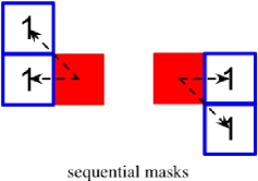
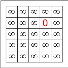
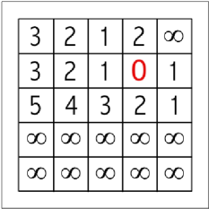
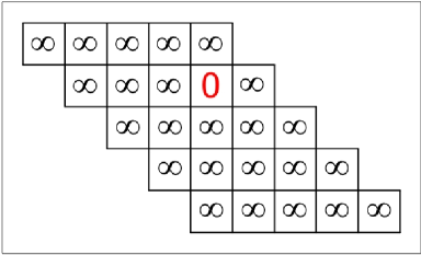
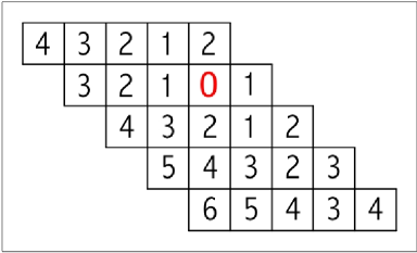
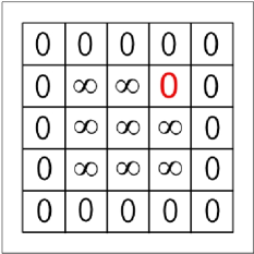
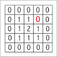
Figure 5: Consider the mask $\mathcal{C}=\{((-1,0),1),((-1,1),1),((1,0),1),((1,-1),1)\}$ (a). The image in (b) is not wedge-preserving when using this mask. In (c), the result of the chamfer algorithm using $\mathcal{C}_{1}=\{((-1,0),1),((-1,1),1)\}$ and $\mathcal{C}_{2}=\{((1,0),1),((1,-1),1)\}$ is shown. By considering the wedge-preserving image in (d), the correct distance map (shown in (e)) is produced. By assigning all border points to the background, the image in (f) is achieved and the chamfer algorithm produces the correct result shown in (g).

Theorem 3.1

If either

• for all border points ${\mathbf{p}}\in\mathcal{S},{\mathbf{p}}\in\overline{X}$ or

• $\mathcal{S}$ is wedge-preserving,

then the chamfer algorithm in Definition 3.5 produces distance maps as defined in Definition 2.6.

Proof.  Let ${\mathbf{p}}\in X$ and ${\mathbf{q}}\in\overline{X}$ be such that $d({\mathbf{p}},{\mathbf{q}})=d({\mathbf{p}},\overline{X})$ and $\mathcal{I}=\left\{i:\left({\overrightarrow{\mathbf{v}}}_{i},w_{i}\right)\in\mathcal{C}\right\}$. There is a set $\{\alpha_{i}\in\mathcal{R}\}$ such that the point ${\mathbf{p}}$ can be written $\displaystyle{\mathbf{p}}={\mathbf{q}}+\sum_{i\in\mathcal{I}}\alpha_{i}{\overrightarrow{\mathbf{v}}}_{i}$ and $\displaystyle d({\mathbf{p}},{\mathbf{q}})=\sum_{i\in\mathcal{I}}\alpha_{i}w_{i}$.

Let $f$ be the image after the first scan. By Lemma 3.1, using that the masks support the scanning order, the local distances are propagated in the following way. Also, by Lemma 3.2 and Lemma 3.3, all points below are in $\mathcal{S}$.

$$f({\mathbf{q}}+{\overrightarrow{\mathbf{v}}}_{k_{1}})= w_{k_{1}} k_{1}$$ for any such that

$${\overrightarrow{\mathbf{v}}}_{k_{1}}\in\mathcal{C}_{1}\textrm{, and }\alpha_{k_{1}}\geq 1$$

$$f({\mathbf{q}}+{\overrightarrow{\mathbf{v}}}_{k_{1}}+{\overrightarrow{\mathbf{v}}}_{k_{2}})= w_{k_{1}}+w_{k_{2}} k_{1} k_{2}$$ for any , such that

$${\overrightarrow{\mathbf{v}}}_{k_{1}},{\overrightarrow{\mathbf{v}}}_{k_{2}}\in\mathcal{C}_{1}$$

$$\textrm{ and }\alpha_{k_{1}},\alpha_{k_{2}}\geq 1$$

$$(\alpha_{k_{1}}\geq 2\textrm{ if }k_{1}=k_{2}),$$

$$\vdots$$

$$\displaystyle f\left({\mathbf{q}}+\sum_{k_{i}:{\overrightarrow{\mathbf{v}}}_{k_{i}}\in\mathcal{C}_{1}}\alpha_{k_{i}}{\overrightarrow{\mathbf{v}}}_{k_{i}}\right)= \displaystyle\sum_{k_{i}:w_{k_{i}}\in\mathcal{C}_{1}}\alpha_{k_{i}}w_{k_{i}}.$$

Let $g$ be the image after the second scan. Using the notation $\displaystyle{\mathbf{q}}_{N}={\mathbf{q}}+\sum_{k_{i}:{\overrightarrow{\mathbf{v}}}_{k_{i}}\in\mathcal{C}_{1}}\alpha_{k_{i}}{\overrightarrow{\mathbf{v}}}_{k_{i}}$, we get

$$g({\mathbf{q}}_{N}+{\overrightarrow{\mathbf{v}}}_{l_{1}})= g({\mathbf{q}}_{N})+w_{l_{1}} l_{1}$$ for any such that

$${\overrightarrow{\mathbf{v}}}_{l_{1}}\in\mathcal{C}_{2}\textrm{, and }\alpha_{l_{1}}\geq 1$$

$$g({\mathbf{q}}_{N}+{\overrightarrow{\mathbf{v}}}_{l_{1}}+{\overrightarrow{\mathbf{v}}}_{l_{2}})= g({\mathbf{q}}_{N})+w_{l_{1}}+w_{l_{2}} l_{1} l_{2}$$ for any , such

$$\textrm{that }{\overrightarrow{\mathbf{v}}}_{l_{1}},{\overrightarrow{\mathbf{v}}}_{l_{2}}\in\mathcal{C}_{2}$$

$$\textrm{and }\alpha_{l_{1}},\alpha_{l_{2}}\geq 1$$

$$(\alpha_{l_{1}}\geq 2\textrm{ if }l_{1}=l_{2})$$

$$\vdots$$

$$\displaystyle g\left({\mathbf{q}}_{N}+\sum_{l_{i}:{\overrightarrow{\mathbf{v}}}_{l_{i}}\in\mathcal{C}_{1}}\alpha_{l_{i}}{\overrightarrow{\mathbf{v}}}_{l_{i}}\right)= g({\mathbf{q}}_{N})+\displaystyle\sum_{l_{i}:w_{l_{i}}\in\mathcal{C}_{2}}\alpha_{l_{i}}w_{l_{i}}= \sum\alpha_{i}w_{i}.$$

This proves that all steps of a shortest path between ${\mathbf{p}}$ and ${\mathbf{q}}$ have been processed. Indeed, after the second scan, the value of the point ${\mathbf{p}}$ is $g({\mathbf{p}})=d({\mathbf{p}},{\mathbf{q}})=\sum\alpha_{i}w_{i}$. $\blacksquare$

Remark 3.3   In Figure 5, the need for the conditions in Theorem 3.1 are shown in example images. $\blacklozenge$

4 Best weights for the BCC and FCC grids

The BCC grid ($\mathbb{B}$) and the FCC grid ($\mathbb{F}$) are defined as follows:

$$\mathbb{B}=\{{\mathbf{p}}(x,y,z)\in\mathbb{Z}^{3}\textrm{ and }x\equiv y\equiv z\pmod{2}\}\textrm{ and}$$

$$\mathbb{F}=\{{\mathbf{p}}(x,y,z)\in\mathbb{Z}^{3}\textrm{ and }x+y+z\equiv 0\pmod{2}\}.$$

A voxel is defined as the Voronoi region of a point ${\mathbf{p}}$ in a grid. Figure 6 (a) shows a voxel of a BCC grid. A BCC voxel has two kinds of face-neighbors (but no edge- or vertex-neighbors), which results in the 8-neighborhood (Figure 6 (b)) and the 14-neighborhood (Figure 6 (c)). On the FCC grid, each voxel (see Figure 6 (d)) has 12 face-neighbors and 6 vertex-neighbors. The resulting 12- and 18-neighborhoods are shown in (Figure 6 (e)) and (Figure 6 (f)), respectively.

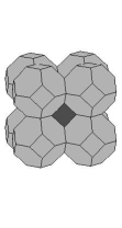
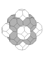
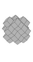
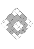
Figure 6: Different neighborhoods for the BCC grid ((a)-(c)) and the FCC grid ((d)-(f)).

Note that the high number of face neighbors (12 for the FCC grid and 14 for the BCC grid) implies these grids are more compact than the cubic grid, which has only $6$ face neighbors.

4.1 Results of the previous sections applied to BCC grids

To apply the results of Sections 2.3 and 3 to the BCC grid, we should check that:

• $\mathbb{B}$ is a sub-module of $\mathbb{R}^{3}$

• Masks decomposed in $\mathbb{B}$-basis wedges can be created

• A scanning order can be defined on the BCC lattice.

Lemma 4.1

Let $\mathbb{B}^{n}=\{{\mathbf{p}}:p^{1},p^{2},...,p^{n}\in\mathbb{Z}\textrm{ and }p^{1}\equiv p^{2}\equiv...\equiv p^{n}\pmod{2}\}$ , then $\left(\mathbb{B}^{n},\mathbb{Z},+,\times\right)$ is a sub-module of $\mathbb{R}^{n}$.

Proof.  Let us prove first that $\mathbb{B}^{n}$ is an Abelian group. Given ${\mathbf{p}}$, ${\mathbf{q}}\in\mathbb{B}^{n}$, there exist $\alpha_{2},...,\alpha_{n}$, and $\beta_{2},...,\beta_{n}\in\mathbb{Z}$ such that $\forall k\in[2..n]\ p^{k}=p^{1}+2\alpha_{k}$ and $q^{k}=q^{1}+2\beta_{k}$. The point ${\mathbf{r}}={\mathbf{p}}+{\mathbf{q}}={\mathbf{q}}+{\mathbf{p}}$ also belongs to $\mathbb{B}^{n}$. Indeed, $\forall k\in[2..n]$, $r^{k}=p^{k}+q^{k}=p^{1}+2\alpha_{k}+q^{1}+2\beta_{k}=r^{1}+2\gamma_{k}$ with $\gamma_{k}=\alpha_{k}+\beta_{k}\in\mathbb{Z}$. Moreover, $-{\mathbf{p}}\in\mathbb{B}^{n}$ as $-p^{k}=-p^{1}+2(-\alpha_{k})$ with $-\alpha_{k}\in\mathbb{Z}$. We now have to prove that $\forall\lambda\in\mathbb{Z}$, $\forall{\mathbf{p}}\in\mathbb{B}^{n}$, $\lambda\cdot{\mathbf{p}}\in\mathbb{B}^{n}$. Indeed, $\forall k\in[1..n],\lambda p^{k}\in\mathbb{Z}$ and $\forall k\in[2..n]\lambda p^{k}=\lambda p^{1}+2(\lambda\alpha_{k})\textrm{ with }(\lambda\alpha_{k})\in\mathbb{Z}$. $\blacksquare$
This result is true for all $n\in\mathbb{N}\setminus\{0\}$ and obviously for $n=3$.

4.1.1 Chamfer mask geometry

Lemma 4.2

A family $\mathcal{F}=\left({\overrightarrow{\mathbf{v}}}_{1},{\overrightarrow{\mathbf{v}}}_{2},{\overrightarrow{\mathbf{v}}}_{3}\right)$ is a basis of $\mathbb{B}$ iff

$$\Delta_{\mathcal{F}}^{0}=\det({\overrightarrow{\mathbf{v}}}_{1},{\overrightarrow{\mathbf{v}}}_{2},{\overrightarrow{\mathbf{v}}}_{3})=\pm 4.$$

Proof.  First, we prove that any determinant of 3 vectors ${\overrightarrow{\mathbf{v}}}_{1},{\overrightarrow{\mathbf{v}}}_{2},{\overrightarrow{\mathbf{v}}}_{3}$ of $\mathbb{B}$ is a multiple of $4$. Indeed, given a vector ${\overrightarrow{\mathbf{v}}}_{i}(x_{i},y_{i},z_{i})$, ${\overrightarrow{\mathbf{v}}}_{i}\in\mathbb{B}$ iff there exists $\alpha_{i},\beta_{i}\in\mathbb{Z}$ such that $y_{i}=x_{i}+2\alpha_{i}$ and $z_{i}=x_{i}+2\beta_{i}$. Then the determinant of ${\overrightarrow{\mathbf{v}}}_{1},{\overrightarrow{\mathbf{v}}}_{2}$ and ${\overrightarrow{\mathbf{v}}}_{3}$ is

$$\begin{array}[]{l c c c}\det({\overrightarrow{\mathbf{v}}}_{1},{\overrightarrow{\mathbf{v}}}_{2},{\overrightarrow{\mathbf{v}}}_{3})&=&\left|\begin{array}[]{c c c}x_{1}&x_{2}&x_{3}\\ y_{1}&y_{2}&y_{3}\\ z_{1}&z_{2}&z_{3}\\ \end{array}\right|&=\left|\begin{array}[]{c c c}x_{1}&x_{2}&x_{3}\\ x_{1}+2\alpha_{1}&x_{2}+2\alpha_{2}&x_{3}+2\alpha_{3}\\ x_{1}+2\beta_{1}&x_{2}+2\beta_{2}&x_{3}+2\beta_{3}\\ \end{array}\right|\\ &=4&\underbrace{\left|\begin{array}[]{c c c}x_{1}&x_{2}&x_{3}\\ \alpha_{1}&\alpha_{2}&\alpha_{3}\\ \beta_{1}&\beta_{2}&\beta_{3}\\ \end{array}\right|}&\\ &&\in\mathbb{Z}&\\ \end{array}.$$

With the notations of paragraph 2.3 we obtain for any vector ${\overrightarrow{\mathbf{v}}}(x,y,z)=(x,x+2\alpha,x+2\beta)$ of $\mathbb{B}$:

$$\frac{1}{\Delta_{\mathcal{F}}^{0}}\times\Delta_{\mathcal{F}}^{1}({\overrightarrow{\mathbf{x}}})=\frac{1}{4\left|\begin{array}[]{c c c}x_{1}&x_{2}&x_{3}\\ \alpha_{1}&\alpha_{2}&\alpha_{3}\\ \beta_{1}&\beta_{2}&\beta_{3}\\ \end{array}\right|}\times 4\left|\begin{array}[]{c c c}x&x_{2}&x_{3}\\ \alpha&\alpha_{2}&\alpha_{3}\\ \beta&\beta_{2}&\beta_{3}\\ \end{array}\right|$$

and $\frac{1}{\Delta_{\mathcal{F}}^{0}}\times\Delta_{\mathcal{F}}^{1}({\overrightarrow{\mathbf{x}}})\in\mathbb{Z}$ iff $\left|\begin{array}[]{c c c}x_{1}&x_{2}&x_{3}\\ \alpha_{1}&\alpha_{2}&\alpha_{3}\\ \beta_{1}&\beta_{2}&\beta_{3}\\ \end{array}\right|=\pm 1$ which means $\Delta_{\mathcal{F}}^{0}=\pm 4$. The same result applies for $\frac{1}{\Delta_{\mathcal{F}}^{0}}\times\Delta_{\mathcal{F}}^{2}({\overrightarrow{\mathbf{x}}})$ and $\frac{1}{\Delta_{\mathcal{F}}^{0}}\times\Delta_{\mathcal{F}}^{3}({\overrightarrow{\mathbf{x}}})$. By Lemma 2.1 we obtain $\mathcal{F}$ is a basis of $\mathbb{B}$ iff $\Delta_{\mathcal{F}}^{0}=\pm 4$. $\blacksquare$

To compute a weighted distance map on an image stored on a BCC grid, one can consider a mask built using 8-neighbors:

$$\mathcal{C}_{8}=\left\{({\overrightarrow{\mathbf{v}}}_{i}(\pm 1,\pm 1,\pm 1),w_{1}),\right\}$$

This mask contains only one type of weight as the Euclidean distance between each face-sharing neighbor to the central voxel is the same.

This mask can be decomposed into $\mathbb{B}$-basis sectors. Indeed, let us consider the wedge $\mathcal{F}_{\mathbb{B}}=\langle\langle{\overrightarrow{\mathbf{v}}}_{1}(1,1,1),{\overrightarrow{\mathbf{v}}}_{2}(-1,1,1),{\overrightarrow{\mathbf{v}}}_{3}(1,-1,1)\rangle\rangle$, and its symmetric wedges.

$$\Delta_{\mathcal{F}_{\mathbb{B}}}^{0}=\det({\overrightarrow{\mathbf{v}}}_{1},{\overrightarrow{\mathbf{v}}}_{2},{\overrightarrow{\mathbf{v}}}_{3})=\left|\begin{array}[]{c c c}1&-1&1\\ 1&1&-1\\ 1&1&1\\ \end{array}\right|=4$$

and from Lemma 4.2, $\mathcal{F}_{\mathbb{B}}$ is a $\mathbb{B}$-basis sector.

If we want larger masks, we can split the wedge $\mathcal{F}_{\mathbb{B}}$ and its symmetric wedges according to the Farey triangulation technique [31, 30]. To do so, given a $\mathbb{B}$-basis wedge $\mathcal{F}=\langle\langle{\overrightarrow{\mathbf{v}}}_{1},{\overrightarrow{\mathbf{v}}}_{2},{\overrightarrow{\mathbf{v}}}_{3}\rangle\rangle$, choose an edge to be split, say the edge between ${\overrightarrow{\mathbf{v}}}_{1}$ and ${\overrightarrow{\mathbf{v}}}_{2}$. We create ${\overrightarrow{\mathbf{v}}}(x,y,z)$ such that ${\overrightarrow{\mathbf{v}}}={\overrightarrow{\mathbf{v}}}_{1}\oplus{\overrightarrow{\mathbf{v}}}_{2}$ defined by $x=x_{1}+x_{2}$, $y=y_{1}+y_{2}$ and $z=z_{1}+z_{2}$. The two obtained wedges $\mathcal{F}_{1}=\langle\langle{\overrightarrow{\mathbf{v}}},{\overrightarrow{\mathbf{v}}}_{2},{\overrightarrow{\mathbf{v}}}_{3}\rangle\rangle$ and $\mathcal{F}_{2}=\langle\langle{\overrightarrow{\mathbf{v}}}_{1},{\overrightarrow{\mathbf{v}}},{\overrightarrow{\mathbf{v}}}_{3}\rangle\rangle$ are $\mathbb{B}$-basis sectors. Indeed,

$$\begin{array}[]{l c l}\Delta_{\mathcal{F}_{1}}^{0}&=&\det({\overrightarrow{\mathbf{v}}},{\overrightarrow{\mathbf{v}}}_{2},{\overrightarrow{\mathbf{v}}}_{3})=\left|\begin{array}[]{c c c}x_{1}+x_{2}&x_{2}&x_{3}\\ y_{1}+y_{2}&y_{2}&y_{3}\\ z_{1}+z_{2}&z_{2}&z_{3}\\ \end{array}\right|=\left|\begin{array}[]{c c c}x_{1}&x_{2}&x_{3}\\ y_{1}&y_{2}&y_{3}\\ z_{1}&z_{2}&z_{3}\\ \end{array}\right|+\left|\begin{array}[]{c c c}x_{2}&x_{2}&x_{3}\\ y_{2}&y_{2}&y_{3}\\ z_{2}&z_{2}&z_{3}\\ \end{array}\right|\\ &=&\Delta_{\mathcal{F}}^{0}=\pm 4.\\ \end{array}$$

In the same way, $\Delta_{\mathcal{F}_{2}}^{0}=\pm 4$.

If we apply the first steps of this method, we can retrieve the chamfer mask using the 14-neighborhood proposed by [27]. But we can also build larger masks by splitting the new wedges.

4.1.2 Chamfer mask weights

To compute optimal integer chamfer weights for BCC grid the depth-first search method of [31, 42] can be used. This method computes weights sets leading to weighted distance maps with small relative error with respect to the corresponding Euclidean map. Moreover, it keeps a weights set only if the normalized polytope of the corresponding mask is convex, which allows application of the results from Section 2.3.

The following tables give sets of integer chamfer mask weights for BCC grids with the scale factor allowing comparison of the final weighted distance map with an Euclidean one composed with real numbers. They also give the maximum relative error that can occur between the weighted distance map and the Euclidean one.

For the two first cases, we also give the optimal real weights computed using the equations of Section 2.4.

Balls obtained by using different number of weights (shown in bold below) are shown in Figure 7.

1. One weight
   For the mask corresponding to the 8-neighborhood, using only one weight, the equations of section 2.4 give the following result:
   real optimal weight 1.268 real optimal error (%) 26.79 integer optimal weight 1 real map scale factor 1.268
   These results are consistent with [27].
   

2. Two weights
   vector weight real weights (1 1 1) $w_{1}$ 1.547 1 2 3 4 5 6 13 19 (2 0 0) $w_{2}$ 1.786 2 3 4 5 6 7 15 22 Scale factor 1 1.268 0.731 0.504 0.383 0.308 0.256 0.119 0.081 Error (%) 10.69 26.79 15.59 12.70 11.60 11.07 10.78 10.72 10.71
    
   

3. Three weights
   vector weight weights (1 1 1) $w_{1}$ 1 2 4 5 6 13 19 26 33 (2 0 0) $w_{2}$ 2 2 5 6 7 15 22 30 38 (2 2 0) $w_{3}$ 2 3 7 8 10 22 31 43 54 Scale factor 1.268 0.899 0.396 0.325 0.270 0.125 0.0857 0.0626 0.0494 Error (%) 26.79 10.10 8.50 7.94 6.39 6.34 6.12 6.12 6.11 Optimal error (%): 6.02
   

   Note: for the previous masks, we displayed real optimal weights to be able to compare our results with previous papers. However, as real optimal weights are computed sector by sector, they may change from one sector to another for the same mask vector. We do not display them for several sectors as they may not be consistent.
   

4. Four weights
   vector weight weights (1 1 1) $w_{1}$ 1 2 4 5 6 9 15 26 (2 0 0) $w_{2}$ 2 2 4 6 7 10 17 29 (2 2 0) $w_{3}$ 2 3 6 8 10 14 24 41 (3 1 1) $w_{4}$ 3 4 7 10 12 17 29 50 Scale factor 1.268 0.899 0.460 0.334 0.275 0.194 0.113 0.0662 Error (%) 26.79 10.10 7.94 5.57 4.73 4.21 4.00 3.99 Optimal error (%): 3.96
   

4.2 Results of previous sections applied to FCC grids

To apply the results of Sections 2.3 and 3 to the FCC grid, we should again check that:

• $\mathbb{F}$ is a sub-module of $\mathbb{R}^{3}$

• Masks decomposed in $\mathbb{F}$-basis wedges can be created

• A scanning order can be defined on the FCC lattice.

The calculations are similar to those in Section 4.1.

Lemma 4.3

Let $\mathbb{F}^{n}=\{{\mathbf{p}}:p^{1},p^{2},...,p^{n}\in\mathbb{Z}\textrm{ and }p^{1}+p^{2}+p^{3}\equiv 0\pmod{2}\}$ , then $\left(\mathbb{F}^{n},\mathbb{Z},+,\cdot\right)$ is a sub-module of $\mathbb{R}^{n}$.

Lemma 4.4

A family $\mathcal{F}=\left({\overrightarrow{\mathbf{v}}}_{1},{\overrightarrow{\mathbf{v}}}_{2},{\overrightarrow{\mathbf{v}}}_{3}\right)$ is a basis of $\mathbb{F}$ iff

$$\Delta_{\mathcal{F}}^{0}=\det({\overrightarrow{\mathbf{v}}}_{1},{\overrightarrow{\mathbf{v}}}_{2},{\overrightarrow{\mathbf{v}}}_{3})=\pm 2.$$

These Lemmas can be proved similar to Lemma 4.1 and 4.2 by noting that for any ${\mathbf{p}}\in\mathbb{F}^{n}$, there exist $\alpha\in\mathbb{Z}$ such that $p^{n}=p^{1}+\dots+p^{n-1}+2\alpha$.

To compute the weighted distance on FCC, we first consider the smallest mask, i.e., the mask containing 12-neighbors:

$$\mathcal{C}_{12}=\left\{({\overrightarrow{\mathbf{v}}}_{i}(\pm 1,\pm 1,0),w_{1}),({\overrightarrow{\mathbf{v}}}_{i}(\pm 1,0,\pm 1),w_{1}),({\overrightarrow{\mathbf{v}}}_{i}(0,\pm 1,\pm 1),w_{1}),\right\}$$

The wedges $\mathcal{F}_{\mathbb{F}}^{1}=\langle\langle{\overrightarrow{\mathbf{v}}}_{1}(1,1,0),{\overrightarrow{\mathbf{v}}}_{2}(1,0,1),{\overrightarrow{\mathbf{v}}}_{3}(1,-1,0)\rangle\rangle$,
$\mathcal{F}_{\mathbb{F}}^{2}=\langle\langle{\overrightarrow{\mathbf{v}}}_{1}(1,1,0),{\overrightarrow{\mathbf{v}}}_{2}(1,0,1),{\overrightarrow{\mathbf{v}}}_{4}(2,0,0)\rangle\rangle$, and their symmetric wedges are $\mathbb{F}$-basis sectors.

$$\Delta_{\mathcal{F}^{1}_{\mathbb{F}}}^{0}=\Delta_{\mathcal{F}^{2}_{\mathbb{F}}}^{0}=2$$

and from Lemma 4.4, $\mathcal{F}_{\mathbb{F}}^{1}$ and $\mathcal{F}_{\mathbb{F}}^{2}$ are $\mathbb{F}$-basis sectors.

The splitting of the sectors are analogous to Section 4.1.1, but the determinants equals $\pm 2$ instead of $\pm 4$.

We get the following mask weights. Balls obtained by using different number of weights (shown in bold below) are shown in Figure 7.

1. One weight
   For the mask corresponding to the 8-neighborhood, using only one weight, the equations of section 2.4 give the following result:
   real optimal weight 1.172 real optimal error (%) 17.16 integer optimal weight 1 real map scale factor 1.172
   These results are consistent with [27].
   

2. Two weights
   vector weight real weights (1 1 0) $w_{1}$ 1.271 1 1 2 (2 0 0) $w_{2}$ 1.798 1 2 3 Scale factor 1 1.464 1.172 0.636 Error (%) 10.10 26.79 17.16 10.10
    
   

3. Three weights
   vector weight weights (1 1 0) $w_{1}$ 1 1 2 2 4 6 7 11 15 (2 0 0) $w_{2}$ 1 2 3 3 6 9 10 16 22 (2 1 1) $w_{3}$ 2 2 3 4 7 10 12 19 26 Scale factor 1.464 1.172 0.694 0.636 0.325 0.226 0.191 0.121 0.0887 Error (%) 26.79 17.16 15.04 10.10 7.94 7.76 6.19 6.16 5.95 Optimal error (%): 5.93
    
   

4. Four weights
   vector weight weights (1 1 0) $w_{1}$ 1 1 2 3 5 5 9 12 (2 0 0) $w_{2}$ 2 2 3 4 7 7 13 17 (2 1 1) $w_{3}$ 2 2 4 5 9 9 16 21 (2 2 2) $w_{4}$ 2 3 5 7 12 13 23 30 Scale factor 1.268 1.172 0.651 0.472 0.274 0.272 0.150 0.113 Error (%) 26.79 17.16 7.94 5.57 5.15 4.64 4.63 4.07 Optimal error (%): 3.98
   

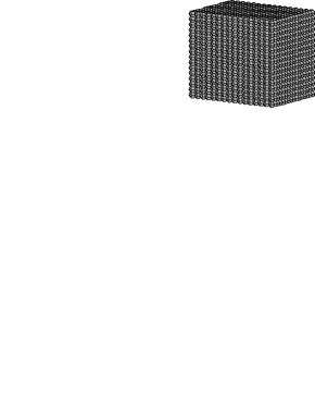
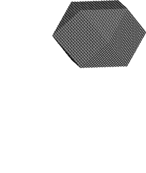
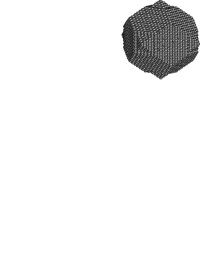
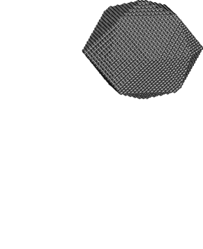
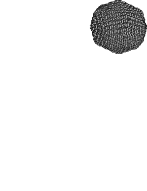
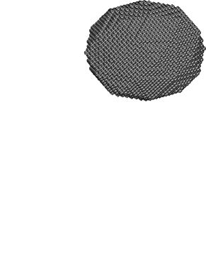
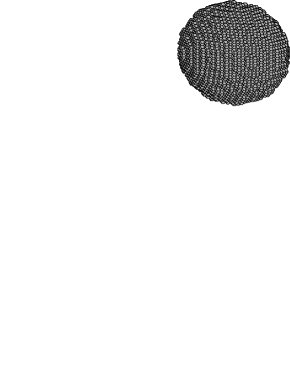
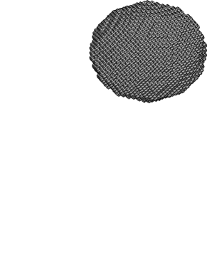
Figure 7: The balls are constructed using the chamfer algorithm in Section 3. Figure (a)–(d) show BCC balls with one (a), two (b), three (c), and four (d) weights. Figure (e)–(h) show FCC balls with one (e), two (f), three (g), and four (h) weights. The weights written in bold in the tables are used. All balls are of radius 20.

5 Conclusions

We have presented a general theory for weighted distances. This allows application of the weighted distance transform to any point-lattice. The optimal weight calculation and the construction of a chamfer algorithm to produce distance maps are straight-forward by the procedure in Section 2.4 and Theorem 3.1. For the chamfer algorithm to construct correct distance-maps, the only limitation is that the image must be wedge-preserving, Definition 3.7, or have all border points in the background, Definition 3.6. With these conditions which can easily be satisfied, images in any dimension can be considered. It is also worth mentioning that despite its popularity, to our knowledge, no proof of the correctness of the two-scan algorithm has been published until now, except for the 2D 3 $\times$ 3 mask algorithm proof from 1966 [12]. Also, the important general formula for the weighted distance between two grid points in Theorem 2.2 is new.

The application of these properties and of the chamfer algorithm are numerous for the cubic and parallelepiped grids in the literature. To illustrate how this theory can be applied, Section 4 gives examples for the FCC and BCC grids. But it can be applied to any point-lattice, for example the 3D grid where the voxels are hexagonal cylinders as suggested in [47] or 4D a grid as in [48], or even other grids as long as they satisfy the module conditions.

References

- [1] G. Borgefors, Applications using distance transforms, in: C. Arcelli, L. P. Cordella, G. Sanniti di Baja (Eds.), Aspects of Visual Form Processing, World Scientific, Singapore, 1994, pp. 83–108.
- [2] C. Pudney, Distance-ordered homotopic thinning: a skeletonization algorithm for 3D digital images, Computer Vision and Image Understanding 72 (3) (1998) 404–413.
- [3] G. Borgefors, Hierarchical chamfer matching: A parametric edge matching algorithm, IEEE Transactions on Pattern Analysis and Machine Intelligence 10 (6) (1988) 849–865.
- [4] G. Herman, J. Zheng, C. Bucholtz, Shape-based interpolation., IEEE Computer Graphics & Applications (1992) 69–79.
- [5] G. Grevera, J. Udupa, Shape-based interpolation of multidimensional grey-level images., IEEE Transactions on Medical Imaging 15 (6) (1996) 881–892.
- [6] J. Cai, J. Chu, D. Recine, M. Sharma, C. Nguyen, R. Rodebaugh, V. Saxena, A. Ali, CT and PET lung image registration and fusion in radiotherapy treatment planning using the chamfer-matching method., International Journal of Radiation Oncology Biology Physics 43 (4) (1999) 883–891.
- [7] S. B. M. Bell, F. C. Holroyd, D. C. Mason, A digital geometry for hexagonal pixels, Image and Vision Computing 7 (3) (1989) 194–204.
- [8] J. H. Conway, N. J. A. Sloane, Sphere Packings, Lattices and Groups, Grundlehren der Mathematischen Wissenschaften 290, Springer-Verlag, New York, 1988.
- [9] L. Ibanez, C. Hamitouche, C. Roux, Determination of discrete sampling grids with optimal topological and spectral properties, in: Proceedings of Conference on Discrete Geometry for Computer Imagery, Lyon, France, Vol. 1176 of Lecture Notes in Computer Science, Springer, 1996, pp. 181–192.
- [10] C. O. S. Sorzano, R. Marabini, J. Velázquez-Muriel, J. R. Bilbao-Castro, S. H. W. Scheres, J. M. Carazo, A. Pascual-Montano, XMIPP: a new generation of an open-source image processing package for electron microscopy, Journal of Structural Biology 148 (2004) 194–204.
- [11] S. Matej, R. M. Lewitt, Efficient 3D grids for image reconstruction using spherically-symmetric volume elements, IEEE Transactions on Nuclear Science 42 (4) (1995) 1361–1370.
- [12] A. Rosenfeld, J. L. Pfaltz, Sequential operations in digital picture processing, Jornal of the ACM 13 (4) (1966) 471–494.
- [13] C. Fouard, G. Malandain, S. Prohaska, M. Westerhoff, F. Cassot, C. Mazel, D. Asselot, J.-P. Marc-Vergnes, Skeletonization by blocks for large datasets: application to brain microcirculation, in: International Symposium on Biomedical Imaging: From Nano to Macro (ISBI’04), IEEE, Arlington, VA, USA, 2004.
- [14] K. Krissian, C.-F. Westin, Fast sub-voxel re-initialization of the distance map for level set methods, Pattern Recognition Letters 26 (10) (2005) 1532–1542.
- [15] J.-B. Lee, J.-H. Lim, C.-W. Park, Development of ethernet based tele-operation systems using haptic devices, Information Sciences 172 (1–2) (2005) 263–280.
- [16] P.-E. Danielsson, Euclidean distance mapping, Computer Graphics and Image Processing 14 (1980) 227–248.
- [17] T. Saito, J.-I. Toriwaki, New algorithms for Euclidean distance transformation of an n-dimensional digitized picture with applications, Pattern Recognition 27 (11) (1994) 1551–1565.
- [18] H. Breu, J. Gil, D. Kirkpatrick, M. Werman, Linear time Euclidean distance transform algorithms, IEEE Transactions on Pattern Analysis and Machine Intelligence 17 (5) (1995) 529–533.
- [19] C. R. Maurer, R. Qi, V. Raghavan, A linear time algorithm for computing exact Euclidean distance transforms of binary images in arbitrary dimensions, IEEE Transactions on Pattern Analysis and Machine Intelligence 25 (2) (2003) 265–270.
- [20] S. Forchhammer, Euclidean distances from chamfer distances for limited distances, in: Proceedings of Scandinavian Conference on Image Analysis (SCIA’89), Oulu, Finland, 1989, pp. 393–400.
- [21] C. Arcelli, G. Sanniti di Baja, Finding local maxima in a pseudo-Euclidean distance transform, Computer Vision, Graphics, and Image Processing 43 (1988) 361–367.
- [22] E. Remy, E. Thiel, Look-up tables for medial axis on squared Euclidean distance transform, in: Proceedings of Conference on Discrete Geometry for Computer Imagery, Naples, Italy, Vol. 2886 of Lecture Notes in Computer Science, Springer, 2003, pp. 224–235.
- [23] E. Remy, E. Thiel, Medial axis for chamfer distances: computing look-up tables and neighbourhoods in 2D or 3D, Pattern Recognition Letters 23 (2001) 649–661.
- [24] P. Nacken, Chamfer metrics in mathematical morphology, Journal of Mathematical Imaging and Vision 4 (1994) 233–253.
- [25] G. Borgefors, Distance transformations in arbitrary dimensions, Computer Vision, Graphics, and Image Processing 27 (1984) 321–345.
- [26] G. Borgefors, Distance transformations on hexagonal grids, Pattern Recognition Letters 9 (1989) 97–105.
- [27] R. Strand, G. Borgefors, Distance transforms for three-dimensional grids with non-cubic voxels, Computer Vision and Image Understanding 100 (3) (2005) 294–311.
- [28] E. Thiel, Géométrie des distance de chanfrein, Habilitation à Diriger des Recherches (2001).
- [29] G. Hardy, E. Wright, An introduction to the theory of numbers, 5th Edition, Oxford University Press, 1978.
- [30] E. Remy, E. Thiel, Optimizing 3D chamfer masks with norm constraints, in: International Workshop on Combinatorial Image Analysis, 2000, pp. 39–56.
- [31] C. Fouard, G. Malandain, 3-D chamfer distances and norms in anisotropic grids, Image and Vision Computing 23 (2) (2005) 143–158.
- [32] E. Remy, Normes de chanfrein et axe médian dans le volume discret., Ph.D. thesis, Université de la Méditerrané, Aix Marseille 2 (December 2001).
- [33] B. Verwer, Distance transforms: metrics, algorithms and applications, Ph.D. thesis, Technische Universiteit, Delft, The Nederlands (1991).
- [34] C. O. Kiselman, Regularity properties of distance transformations in image analysis, Computer Vision and Image Understanding 64 (3) (1996) 390–398.
- [35] P. P. Das, B. N. Chatterji, Knight’s distance in digital geometry, Pattern Recognition 7 (4) (1988) 215–226.
- [36] B. Verwer, Local distances for distance transformaions in two and three dimensions, Pattern Recognition Letters 12 (1991) 671–682.
- [37] G. Borgefors, Distance transformations in digital images, Computer Vision, Graphics, and Image Processing 34 (1986) 344–371.
- [38] S. Svensson, G. Borgefors, Digital distance transforms in 3D images using information from neighbourhoods up to , Computer Vision and Image Understanding 88 (1) (2002) 24–53.
- [39] D. Coquin, P. Bolon, Discrete distance operator on rectangular grids, Pattern Recognition Letters 16 (1998) 911–923.
- [40] J. Mangin, I. Bloch, J. López-Krahe, Chamfer distances in anisotropic 3D images, in: VII European Signal Processing Conference, Edinburgh, UK, 1994, pp. 975–978.
- [41] I. Sintorn, G. Borgefors, Weighted distance transforms for volume images digitized in elongated voxel grids, Pattern Recognition Letters 25 (5) (2004) 571–580.
-
[42]
G. Malandain, C. Fouard, On optimal chamfer masks and coefficients, Research
Report 5566, INRIA, Sophia Antipolis, France (May 2005).
URL http://www.inria.fr/rrrt/rr-5566.html - [43] J. Bresenham, Pixel-processing fundamentals, IEEE Comput. Graph. Appl. 16 (1) (1996) 74–82.
- [44] L. Dorst, A. W. M. Smeulders, Best linear unbiased estimators for properties of digitized straight lines, IEEE Trans. Pattern Anal. Mach. Intell. 8 (2) (1986) 276–282.
- [45] L. Dorst, P. W. Verbeek, The constrained distance transformation: A pseudo-Euclidian, recursive implementation of the lee-algorithm, in: Proc. European Signal Processing Conference 1986, The Hague, The Netherlands, 1986, pp. 917–920.
- [46] A. Rosenfeld, J. L. Pfaltz, Distance functions on digital pictures, Pattern Recognition 1 (1968) 33–61.
- [47] V. E. Brimkov, R. P. Barneva, Analytical honeycomb geometry for raster and volume graphics, The Computer Journal 48 (2) (2005) 180–199.
- [48] G. Borgefors, Weighted digital distance transforms in four dimensions, Discrete Applied Mathematics 125 (1) (2003) 161–176.