The Comprehensive Analysis of Neutrino Events Occurring inside the Detector in the Super-Kamiokande Experiment from the View Point of the Numerical Computer Experiments: Part 1
–Mutual Relation between the Directions of the Incident Neutrinos and those of the Produced Leptons–

Abstract

Super-Kamiokande collaboration assumes that the direction of every observed lepton coincides with the incoming direction of the incident neutrino, which is the fundamental basement throughout all their analysis on neutrino oscillation. We examine whether this assumption to explain the experimental results on neutrino oscillation is theoretically acceptable. Treating every physical process concerned stochastically, we have examined if this assumption just cited is acceptable. As the result of it, we have shown that this assumption does not hold even if statistically.

Keywords: Super-Kamiokande, QEL, Computer Numerical Experiment

1 Introduction: The motivation of the paper

According to the results obtained from the Super-Kamiokande Experiments on atmospheric neutrinos, oscillation phenomena have been found between two neutrinos, $\nu_{\mu}$and $\nu_{\tau}$. Published reports on the confirmation to the oscillation between the neutrinos, $\nu_{\mu}$and $\nu_{\tau}$, and the history forgoing to these experiments will be critically reviewed and details are in the following:

• During 1980’s Kamiokande and IMB observed smaller atmospheric neutrino flux ratio $\nu_{\mu}/\nu_{e}$ than the predicated value [1].

• Kamiokande found anomaly in the zenith angle distribution [2]

• Super-Kamiokande found $\nu_{\mu}$-$\nu_{\tau}$ oscillation [3] and
  Soudan2 and MACRO confirm the Super-Kamiokande result [4].

• K2K, the first accelerator-based long baseline experiment, confirmed atmospheric neutrino oscillation[5].

• MINOS’s precision measurement gives the consistent results with Super-Kamiokande ones[6].

It is well known that Super-Kamiokande Collaboration examined all possible types of the neutrino events, such as, say, Sub-GeV e-like, Multi-GeV e-like, Sub-GeV $\mu$-like, Multi-GeV $\mu$-like, Multi-ring Sub-GeV $\mu$-like, Multi-ring Multi-GeV $\mu$-like, PC, Upward Stopping Muon Events and Upward Through Going Muon Events, in other words, all possible interactions by neutrino, such as, elastic and quasielastic scattering, single-meson production and deep scattering are considered. Furthermore, all topologically different types of neutrino events lead the unified numerical oscillation parameters, say, $\Delta m^{2}=2.4\times 10^{-3}\rm{eV^{2}}$ and $sin^{2}2\theta=1.0$ [12].

Taking into account all factors mentioned above, it is natural that the majority should believe the finding of the $\mu-\tau$ neutrino oscillation by Super-Kamiokande Collaboration.

However, it should be emphasized strongly that the Super-Kamiokande Collaboration put the fundamental assumption in the analysis of the atmospheric neutrino oscillation which is never self-evident and should be carefully examined. This assumption is that the direction of the incident neutrino is the same as that of emitted lepton(s).

In order to avoid any misunderstanding toward the SK assumption on the direction we reproduce this assumption from the original SK papers and their related papers in italic.
Kajita and Totsuka state:

”However, the direction of the neutrino must be estimated from the reconstructed direction of the products of the neutrino interaction. In water Cheren-kov detectors, the direction of an observed lepton is assumed to be the direction of the neutrino. Fig.11 and Fig.12 show the estimated correlation angle between neutrinos and leptons as a function of lepton momentum. At energies below 400 MeV/c, the lepton direction has little correlation with the neutrino direction. The correlation angle becomes smaller with increasing lepton momentum. Therefore, the zenith angle dependence of the flux as a consequence of neutrino oscillation is largely washed out below 400 MeV/c lepton momentum. With increasing momentum, the effect can be seen more clearly.” [7]

On the other hand, Ishitsuka states in his Ph.D thesis which is exclusively devoted into the L/E analysis of the atmospheric neutrino from Super-Kamiokande experiment as follows:

” 8.4 Reconstruction of $L_{\nu}$

Flight length of neutrino is determined from the neutrino incident zenith angle, although the energy and the flavor are also involved. First, the direction of neutrino is estimated for each sample by a different way. Then, the neutrino flight lenght is calclulated from the zenith angle of the reconstructed direction.

8.4.1 Reconstruction of Neutrino Direction

FC Single-ring Sample

The direction of neutrino for FC single-ring sample is simply assumed to be the same as the reconstructed direction of muon. Zenith angle of neutrino is reconstructed as follows:

$$\hskip 56.9055pt\cos\Theta^{rec}_{\nu}=\cos\Theta_{\mu}\hskip 56.9055pt(8.17)$$

,where $\cos\Theta^{rec}_{\nu}$ and $\cos\Theta_{\mu}$ are cosine of the reconstructed zenith angle of neutrino and muon, respectively.” [8]

Furthermore, Jung, Kajita et al. state:

”At neutrino energies of more than a few hundred MeV, the direction of the reconstructed lepton approximately represents the direction of the original neutrino. Hence, for detectors near direction of the lepton. Any effects, such as neutrino oscillations, that are a function of the neutrino flight distance will be manifest in the lepton zenith angle distributions.” [9]

Hereafter, we call the fundamental assumption by the Super-Kamiokande Experiment simply as the SK assumption on the direction.

In section 2, we discuss treatment on the cross section for Quasi-Elastic Scattering(QEL) stochastically which play an particularly important role in the analysis of Fully Contained Events. In section 3, we treat the effect of azimuthal angle of QEL over the zenith angle of the neutrino events which could not be treated in the Detector Simulation carried by the Super-Kaomiokande Collaboration. In section 4, we treat the zenith angle distributions of the neutrino events for the different directions of the incident neutrinos stochastically, taking into account of the corresponding incident neutrino energy spectrum. In section 5, we discuss the correlation diagram between the zenith angles of the incident neutrinos and those of the produced muons, and show that the SK assumption on the direction does not hold even if statistically. As the result of it, for example, upward neutrino zenith angle distribution in the absence of neutrino oscillation does not reproduce the corresponding one of the produced muons. In the conclusion, we state that we will give the results of re-analysis of the $L/E$ distribution obtained by Super-Kamiokande experiment under the situation that the SK assumption on the direction does not hold in the subsequent paper.

2 Cross Sections of Quasi Elastic Scattering in the Neutrino Reaction and the Scattering Angle of Charged Leptons.

In order to examine the validity of the SK assumption on the direction, we consider the following quasielastic scattering(QEL):

$$\nu_{e}+n\longrightarrow p+e^{-}$$

$$\nu_{\mu}+n\longrightarrow p+\mu^{-}$$

$$\bar{\nu}_{e}+p\longrightarrow n+e^{+}$$ (1)

$$\bar{\nu}_{\mu}+p\longrightarrow n+\mu^{+},$$

because the QEL is the most dominant process in Fully Contained Events and Partially Contained Events which occur in the detector. Also, we adopt the QEL events among Fully Contained Events as the object for the analysis, because they are simple and solid events in which the energies of the produced muons (electrons) could be uniquely determined, compared with any other type of the neutrino event. The differential cross section for QEL is given as follows [10].

$$\frac{{\rm d}\sigma_{\ell(\bar{\ell})}(E_{\nu(\bar{\nu})})}{{\rm d}Q^{2}}=\frac{G_{F}^{2}{\rm cos}^{2}\theta_{C}}{8\pi E_{\nu(\bar{\nu})}^{2}}\Biggl{\{}A(Q^{2})\pm B(Q^{2})\biggl{[}\frac{s-u}{M^{2}}\biggr{]}+$$

$$C(Q^{2})\biggl{[}\frac{s-u}{M^{2}}\biggr{]}^{2}\Biggr{\}},$$ (2)

where

$$A(Q^{2}) = \frac{Q^{2}}{4}\Biggl{[}f^{2}_{1}\biggl{(}\frac{Q^{2}}{M^{2}}-4\biggr{)}+f_{1}f_{2}\frac{4Q^{2}}{M^{2}}$$

$$+f_{2}^{2}\biggl{(}\frac{Q^{2}}{M^{2}}-\frac{Q^{4}}{4M^{4}}\biggr{)}+g_{1}^{2}\biggl{(}4+\frac{Q^{2}}{M^{2}}\biggl{)}\Biggr{]},$$

$$B(Q^{2}) = (f_{1}+f_{2})g_{1}Q^{2},$$

$$C(Q^{2}) = \frac{M^{2}}{4}\biggl{(}f^{2}_{1}+f^{2}_{2}\frac{Q^{2}}{4M^{2}}+g_{1}^{2}\biggr{)}.$$

The signs $+$ and $-$ refer to $\nu_{\mu(e)}$ and $\bar{\nu}_{\mu(e)}$ for charged current (c.c.) interactions, respectively. The $Q^{2}$ denotes the four momentum transfer between the incident neutrino and the charged lepton. Details of other symbols are given in [10].

The relation among $Q^{2}$, $E_{\nu(\bar{\nu})}$, the energy of the incident neutrino, $E_{\ell}$, the energy of the emitted charged lepton (muon or electron or their anti-particles) and $\theta_{\rm s}$, the scattering angle of the emitted lepton, is given as

$$Q^{2}=2E_{\nu(\bar{\nu})}E_{\ell}(1-{\rm cos}\theta_{\rm s}).$$ (3)

Also, the energy of the emitted lepton is given by

$$E_{\ell}=E_{\nu(\bar{\nu})}-\frac{Q^{2}}{2M}.$$ (4)

Now, let us examine the magnitude of the scattering angle of the emitted lepton in a quantitative way, as this plays a decisive role in determining the accuracy of the direction of the incident neutrino, which is directly related to the reliability of the zenith angle distribution of both Fully Contained Events and Partially Contained Events in the Super-Kamiokande Experiment.

By using Eqs. (2) to (4), we obtain the distribution function for the scattering angle of the emitted leptons and the related quantities by a Monte Carlo method. The procedure for determining the scattering angle for a given energy of the incident neutrino is described in the Appendix A. Fig. 1 shows this relation for muon, from which we can easily understand that the scattering angle $\theta_{\rm s}$ of the emitted lepton ( muon here ) cannot be neglected. For a quantitative examination of the scattering angle, we construct the distribution function for ${\theta_{\rm s}}$ of the emitted lepton from Eqs. (2) to (4) by using a Monte Carlo method.

Fig. 2 gives the distribution function for $\theta_{\rm s}$ of the muon produced in the muon neutrino interaction. It can be seen that the muons produced from lower energy neutrinos are scattered over wider angles and that a considerable part of them are scattered even in backward directions. Similar results are obtained for anti-muon neutrinos, electron neutrinos and anti-electron neutrinos.

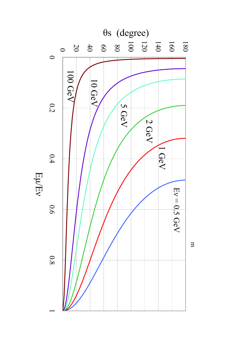
Figure 1: Relation between the energy of the muon and its scattering angle for different incident muon neutrino energies, 0.5, 1, 2, 5, 10 and 100 GeV.

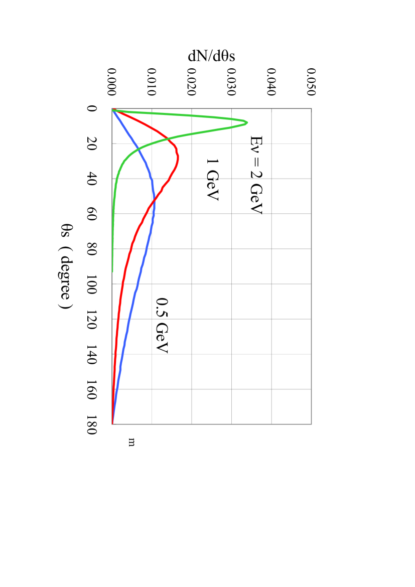
Figure 2: Distribution functions for the scattering angle of the muon for muon-neutrino with incident energies, 0.5 , 1.0 and 2 GeV. Each curve is obtained by the Monte Carlo method (one million sampling per each curve).

Also, in a similar manner, we obtain not only the distribution function for the scattering angle of the charged leptons, but also their average values $<\theta_{\rm s}>$ and their standard deviations $\sigma_{\rm s}$. Table 1 shows them for muon neutrinos, anti-muon neutrinos, electron neutrinos and anti-electron neutrinos. From the Table 1, it seems that the scattering angles could not be neglected. However, Super-Kamiokande Collaboration approximate them as zero, as cited in three passages (in Italic) mentioned above [7],[8],[9]. Or they may claim that such the assumption surely holds statistically as whole (see the Conclusion of our paper, relating to the latter surmise).

Table 1: The average values $<\theta_{\rm s}>$ for scattering angle of the emitted charged leptons and their standard deviations $\sigma_{\rm s}$ for various primary neutrino energies $E_{\nu(\bar{\nu})}$.

$E_{\nu(\bar{\nu})}$ (GeV)	angle	$\nu_{\mu(\bar{\mu})}$	$\bar{\nu}_{\mu(\bar{\mu})}$	$\nu_{e}$	$\bar{\nu_{e}}$
	(degree)
0.2	$<\theta_{\mathrm{s}}>$	89.86	67.29	89.74	67.47
	$\sigma_{\mathrm{s}}$	38.63	36.39	38.65	36.45
0.5	$<\theta_{\mathrm{s}}>$	72.17	50.71	72.12	50.78
	$\sigma_{\mathrm{s}}$	37.08	32.79	37.08	32.82
1	$<\theta_{\mathrm{s}}>$	48.44	36.00	48.42	36.01
	$\sigma_{\mathrm{s}}$	32.07	27.05	32.06	27.05
2	$<\theta_{\mathrm{s}}>$	25.84	20.20	25.84	20.20
	$\sigma_{\mathrm{s}}$	21.40	17.04	21.40	17.04
5	$<\theta_{\mathrm{s}}>$	8.84	7.87	8.84	7.87
	$\sigma_{\mathrm{s}}$	8.01	7.33	8.01	7.33
10	$<\theta_{\mathrm{s}}>$	4.14	3.82	4.14	3.82
	$\sigma_{\mathrm{s}}$	3.71	3.22	3.71	3.22
100	$<\theta_{\mathrm{s}}>$	0.38	0.39	0.38	0.39
	$\sigma_{\mathrm{s}}$	0.23	0.24	0.23	0.24

3 Influence of Azimuthal Angle of Quasi Elastic Scattering over the Zenith Angle of both Fully Contained Events and Partially Contained Events

In the present section, we examine the effect of the azimuthal angles, $\phi$, of the emitted leptons over their own zenith angles, $\theta_{\mu(\bar{\mu}))}$, for given zenith angles of the incident neutrinos, $\theta_{\nu(\bar{\nu}))}$, which could not be considered in the detector simulation carried by the Super-Kamiokande Collaboration.

For three typical cases (vertical, horizontal and diagonal), Fig. 3 gives a schematic representation of the relationship between, $\theta_{\nu(\bar{\nu})}$, the zenith angle of the incident neutrino, and ( $\theta_{\rm s}$, $\phi$), a pair of scattering angle of the emitted lepton and its azimuthal angle.

From Fig. 3(a), it can been seen that the zenith angle $\theta_{\mu(\bar{\mu})}$ of the emitted lepton is not influenced by its $\phi$ in the vertical incidence of the neutrinos $(\theta_{\nu(\bar{\nu})}=0^{\rm o})$, as it must be. From Fig. 3(b), however, it is obvious that the influence of $\phi$ of the emitted leptons on their own zenith angle is the strongest in the case of horizontal incidence of the neutrino $(\theta_{\nu(\bar{\nu})}=90^{\rm o})$. Namely, one half of the emitted leptons are recognized as upward going, while the other half is classified as downward going ones. The diagonal case ( $\theta_{\nu(\bar{\nu})}=43^{\rm o}$) is intermediate between the vertical and the horizontal. In the following, we examine the cases for vertical, horizontal and diagonal incidence of the neutrino with different energies, say, $E_{\nu(\bar{\nu})}=0.5$ GeV, $E_{\nu(\bar{\nu})}=1$ GeV and $E_{\nu(\bar{\nu})}=5$ GeV, as the typical cases.

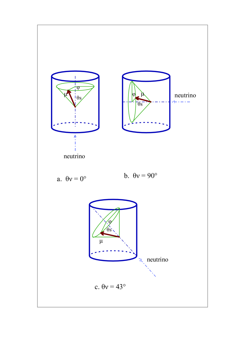
Figure 3: Schematic view of the zenith angles of the charged muons for different zenith angles of the incident neutrinos, focusing on their azimuthal angles.

3.1 Dependence of the spreads of the zenith angle for the emitted leptons on the energies of the emitted leptons for different incident directions of the neutrinos with different energies

The detailed procedure for the Monte Carlo simulation is described in the Appendix A. We give the scatter plots between the fractional energies of the emitted muons and their zenith angle for a definite zenith angles of the incident neutrino with different energies in Figs. 6 to 6. In Fig. 6, we give the scatter plots for vertically incident neutrino with different energies 0.5 GeV, 1 GeV and 5 GeV . In this case, the relations between the emitted energies of the muons and their zenith angles are unique, which comes from the definition of the zenith angle of the emitted lepton. However, the densities (frequencies of the event number) along each curves are different in position to position and depend on the energies of the incident neutrinos. Generally speaking, densities along the curves become greater toward $\cos\theta_{\mu(\bar{\mu})}=1$. In this case, $\cos\theta_{\mu(\bar{\mu})}$ is never influenced by the azimuthal angel in the scattering by the definition .

On the contrast, it is shown in Figure 5 that the horizontally incident neutrinos give the widest zenith angles distribution for the emitted energies of muons due to the effect of their azimuthal angles. The more lower incident neutrino energies, the more wider spread of the emitted leptons. As easily understood from Figure 6, the diagonally incident neutrinos give the intermediate zenith angle distributions for the emitted muons between those for vertically incident neutrinos and those for horizontally neutrinos.

(a)                                            (b)                                            (c)

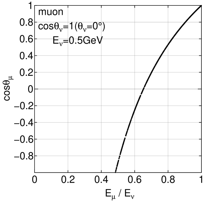
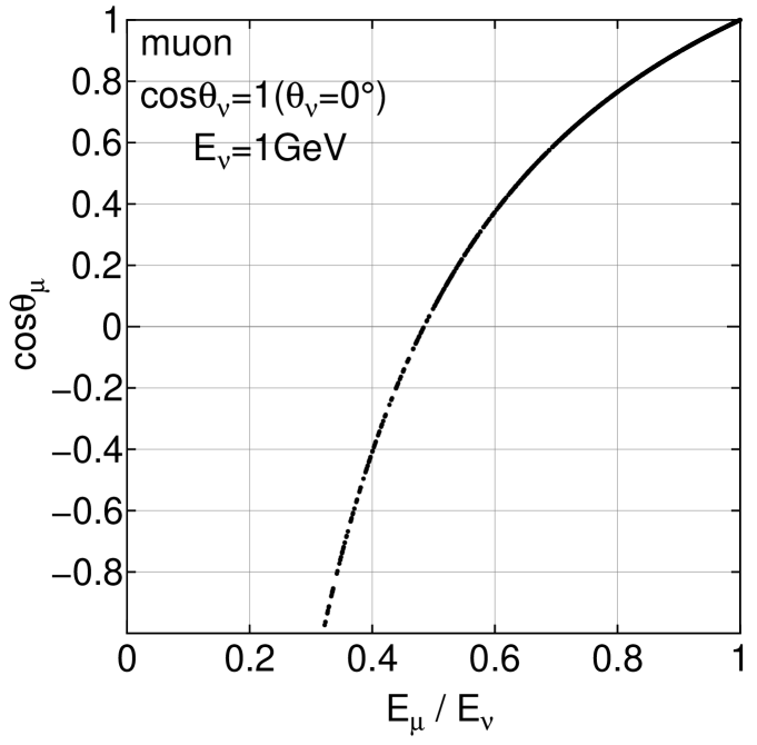
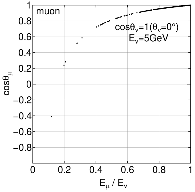
Figure 4: The scatter plots between the fractional energies of the produced muons and their zenith angles for vertically incident muon neutrinos with 0.5 GeV, 1 GeV and 5 GeV, respectively. The sampling number is 1000 for each case.

(a)                                            (b)                                            (c)

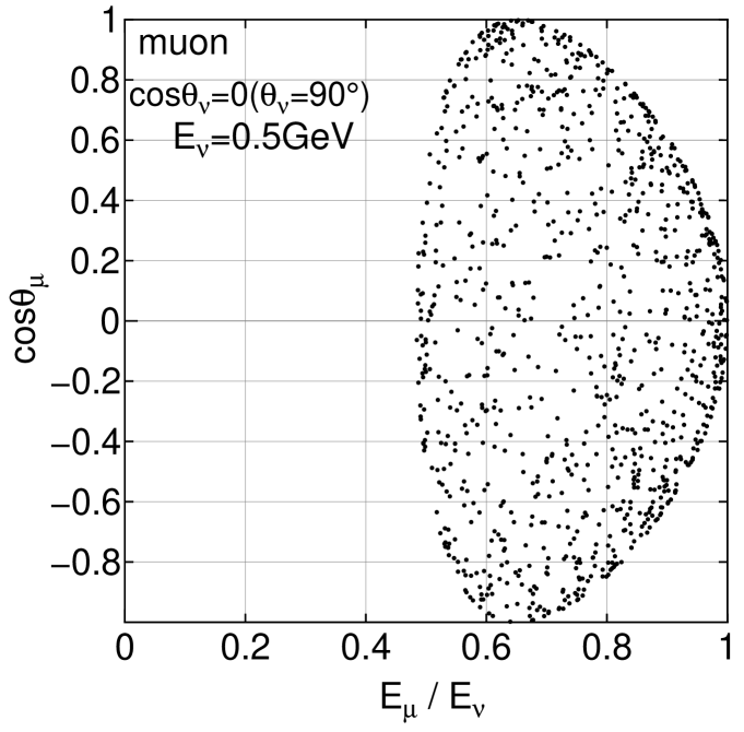
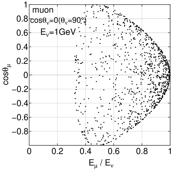
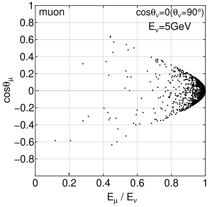
Figure 5: The scatter plots between the fractional energies of the produced muons and their zenith angles for horizontally incident muon neutrinos with 0.5 GeV, 1 GeV and 5 GeV, respectively. The sampling number is 1000 for each case.

(a)                                            (b)                                            (c)

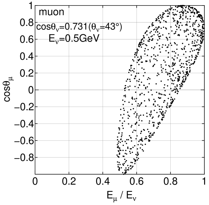
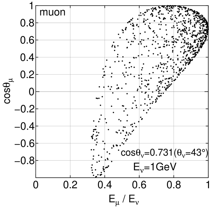
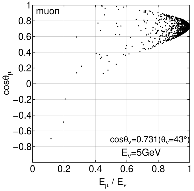
Figure 6: The scatter plots between the fractional energies of the produced muons and their zenith angles for diagonally incident muon neutrinos with 0.5 GeV, 1 GeV and 5 GeV, respectively. The sampling number is 1000 for each case.

(a)                                            (b)                                            (c)

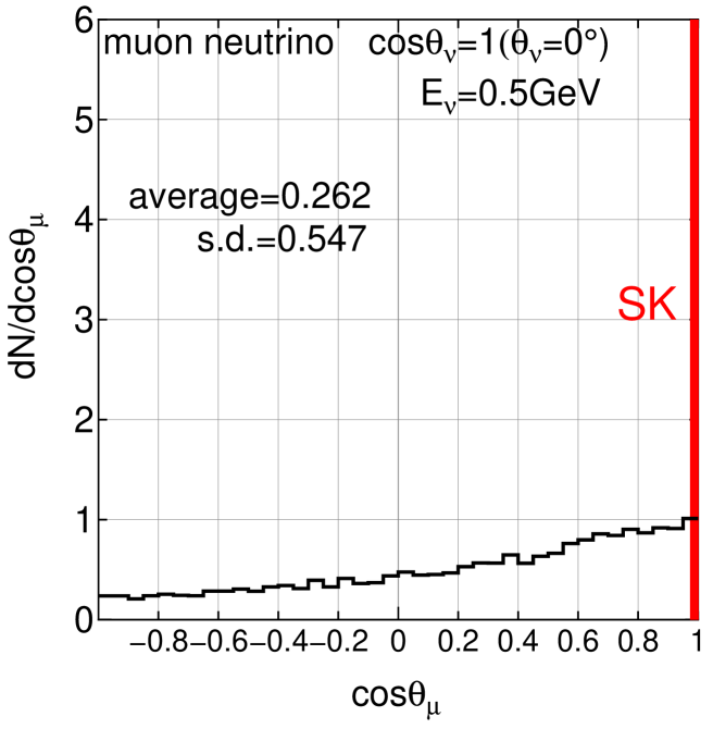
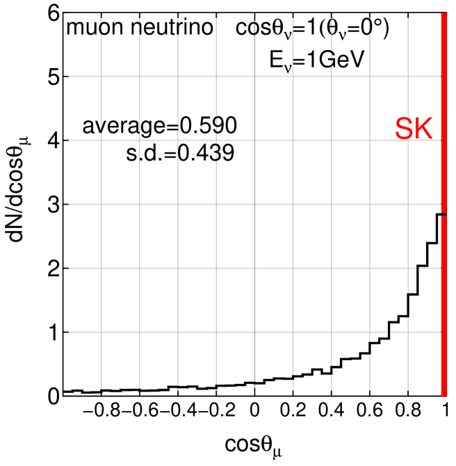
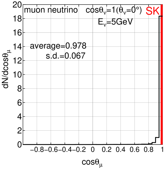
Figure 7: Zenith angle distribution of the muon for the vertically incident muon neutrino with 0.5 GeV, 1 GeV and 5 GeV, respectively. The sampling number is 10000 for each case. SK stands for the corresponding ones under the SK assumption.

(a)                                            (b)                                            (c)

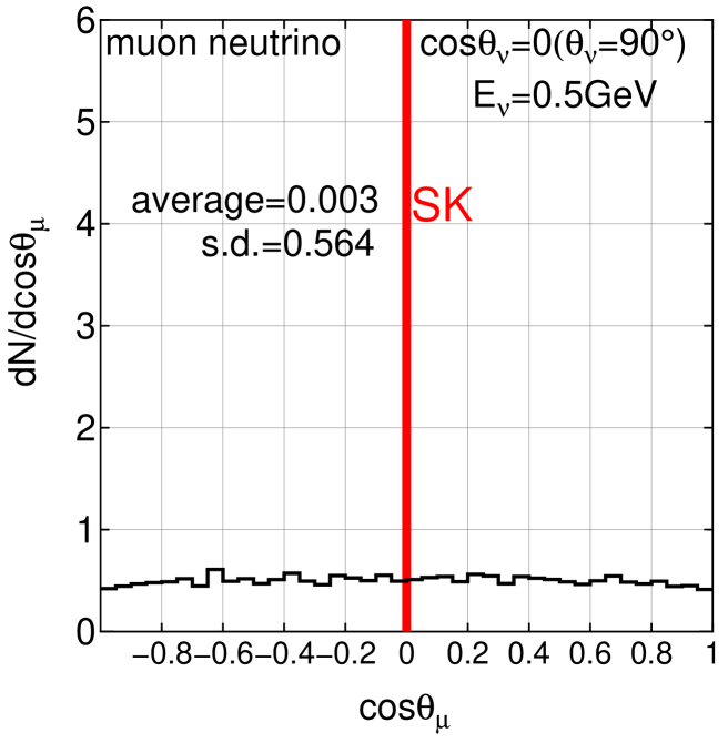
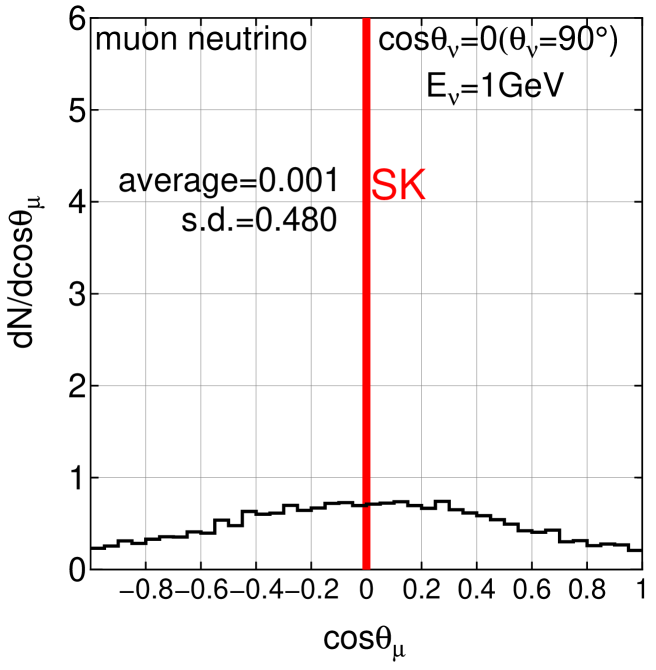
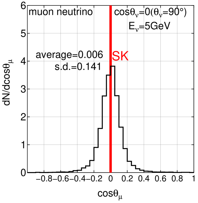
Figure 8: Zenith angle distribution of the muon for the horizontally incident muon neutrino with 0.5 GeV, 1 GeV and 5 GeV, respectively. The sampling number is 10000 for each case. SK stands for the corresponding ones under the SK assumption.

(a)                                            (b)                                            (c)

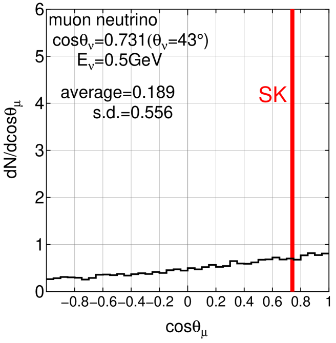
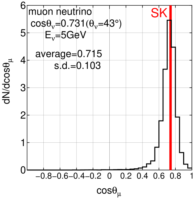
Figure 9: Zenith angle distribution of the muon for the diagonally incident muon neutrino with 0.5 GeV, 1 GeV and 5 GeV, respectively. The sampling number is 10000 for each case. SK stands for the corresponding ones under the SK assumption.

3.2 Zenith angle distribution of the emitted lepton for the different incidence of the neutrinos with different energies

In Figures 7 to 9, we express Figs. 4 to 6 in a different way. We sum up muon events with different emitted energies for given zenith angles. As the result of it, we obtain frequency distribution of the neutrino events as a function of $cos\theta_{\mu}$ for different incident directions and different incident energies of neutrinos.

In Figures 7(a) to 7(c), we give the zenith angle distributions of the emitted muons for the case of vertically incident neutrinos with different energies, say, $E_{\nu}=0.5$ GeV, $E_{\nu}=1$ GeV and $E_{\nu}=5$ GeV.

Comparing the case for 0.5 GeV with that for 5 GeV, we understand the big contrast between them as for the zenith angle distribution. The scattering angle of the emitted muon for 5 GeV neutrino is relatively small (See, Table 1) so that the emitted muons keep roughly the same direction as their original neutrinos. In this case, the effect of their azimuthal angle on the zenith angle is also small. However, in the case for 0.5 GeV which is the dominant energy for Fully Contained Events and Partially Contained Events in the Superkamiokande, there is even a possibility for the emitted muon to be emitted in the backward direction due to the large angle scattering, the effect of which is enhanced by their azimuthal angle.

The most frequent occurrence in the backward direction of the emitted muon appears in the horizontally incident neutrino as shown in Figs. 8(a) to 8(c). In this case, the zenith angle distribution of the emitted muon should be symmetrical to the horizontal direction. Comparing the case for 5 GeV with those both for $\sim$0.5 GeV and for $\sim$1 GeV, even 1 GeV incident neutrinos lose almost the original sense of the incidence if we measure it by the zenith angle of the emitted muon. Figs. 9(a) to 9(c) for the diagonally incident neutrino tell us that the situation for diagonal cases lies between the case for the vertically incident neutrino and that for horizontally incident one. SK in the figures denotes the SK assumption on the direction of incident neutrinos. From the Figures 7(a) to 9(c), it seems to be clear that the scattering angles of emitted muons influence their zenith angles, which is enhanced by their azimuthal angles, particularly more inclined directions of the incident neutrinos.

(a)                                            (b)                                            (c)

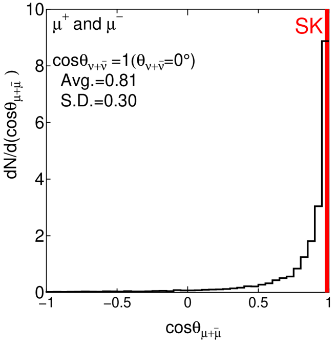
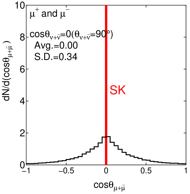
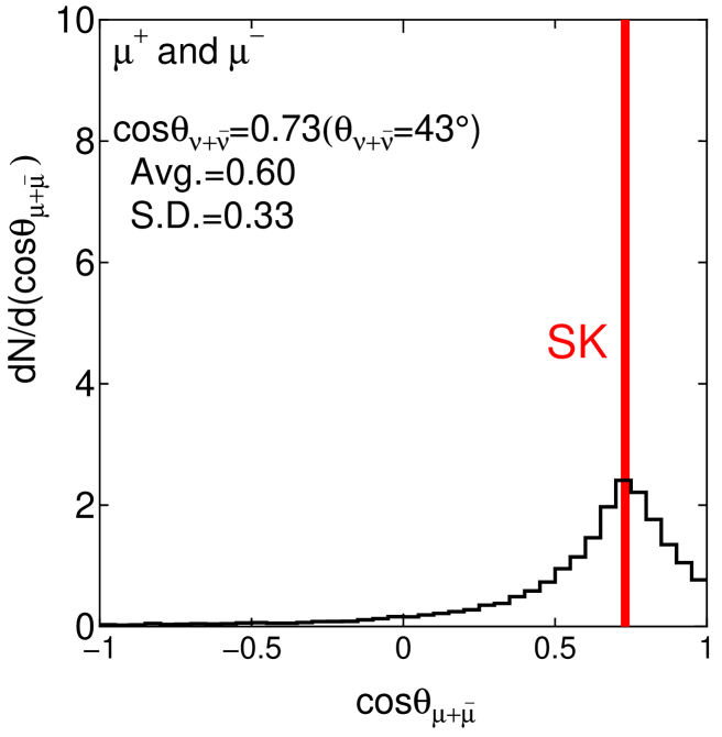
Figure 10: Zenith angle distribution of $\mu^{-}$ and $\mu^{+}$ for $\nu$ and $\bar{\nu}$ for the incident neutrinos with the vertical, horizontal and diagonal directions, respectively (see Figure 3). The overall neutrino spectrum at Kamioka site is taken into account. The sampling number is 10000 for each case. SK stand for the corresponding ones under the SK assumption.

4 Zenith Angle Distribution of Fully Contained Events and Partially Contained Events for a Given Zenith Angle of the Incident Neutrino, Taking Their Energy Spectrum into Account

In the previous sections, we discuss the relation between the zenith angle distribution of the incident neutrino with a single energy and that of the emited muons produced by the neutrino for the different incident direction. In order to apply our motivation around the uncertainty of the SK assumption on the direction for Fully Contained Events and Partially Contained Events, we must consider the effect of the energy spectrum of the incident neutrino. The Monte Carlo simulation procedures for this purpose are given in the Appendix B.

In Fig. 10, we give the zenith angle distributions of the sum of $\mu^{+}(\bar{\mu})$ and $\mu^{-}$ for a given zenith angle of $\bar{\nu}_{\bar{\mu}}$ and $\nu_{\mu}$, taking into account different primary neutrino energy spectra for differnt directions at Kamioka site. SK in the figures denotes the SK assumption on the direction. From the figures, it seems to be clear that the SK assumption on the direction does not hold. Namely, we could conclude that the scattering angle of the emitted muons acompanied by their azimuthal angles influence their zenith angle distribution for the all directions.

5 Correlation between the Zenth Angle Distribution of the Incident Neutrinos and that of the Emitted Leptons

Now, we extend the results for the definite zenith angle obtained in the previous sections to the case in which we consider the zenith angle distribution of the incident neutrinos totally.

Here, we examine the real correlation between ${\cos\theta_{\nu}}$ and ${\cos{\theta}_{\mu}}$, by performing the exact Monte Carlo simulation.

The detail for the simulation procedure is given in the Appendix C.

In order to obtain the zenith angle distribution of the emitted leptons for that of the incident neutrinos, we divide the cosine of the zenith angle of the incident neutrino into twenty regular intervals from $\cos{\theta_{\nu}}=0$ to $\cos{\theta_{\nu}}=1$. For the given interval of $\cos{\theta_{\nu}}$, we carry out the exact Monte Carlo simulation, and obtain the cosine of the zenith angle of the emitted leptons.

Thus, for each interval of $\cos{\theta_{\nu}}$, we obtain the corresponding zenith angle distribution of the emitted leptons. Then, we sum up these corresponding ones over all zenith angles of the incident neutrinos and we finally obtain the relation between the zenith angle distribution for the incident neutrinos and that for the emitted leptons.

In a similar manner, we could obtain between $\cos{\theta_{\bar{\nu}}}$ and $\cos{\theta_{\bar{\mu}}}$ for anti-neutrinos. The situation for anti-
neutrinos is essentially the same as that for neutrinos.

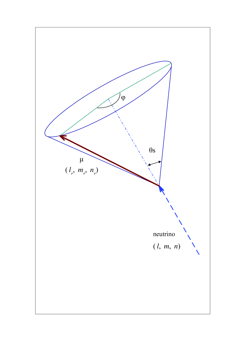
Figure 15: The relation between the direction cosine of the incident neutrino and that of the emitted charged lepton.

In Fig. 11 we classsify the correlation between ${\cos\theta_{\nu}}$ and ${\cos{\theta}_{\mu}}$ according to the different energy range of the incident muon neutrinos. The ${\cos{\theta}_{\mu}}$ distribution along ${\cos\theta_{\nu}}=1$, ${\cos\theta_{\nu}}=0$ and ${\cos\theta_{\nu}}=0.73$ in Figure 11 correspond to Figure 10(a) (vertical), Figure 10(b)(horizontal) and Figure 10(c) (diagonal), respectively. Looking the ${\cos\theta_{\mu}}$ distribution for the fixed ${\cos\theta_{\nu}}$ in the Figure 11, it is well understood that the ${\cos\theta_{\mu}}$ distribution around ${\cos\theta_{\mu}}\approx{\cos\theta_{\nu}}$ spreads wider as ${\cos\theta_{\nu}}$ decreases. This is due to the effect of scattering angle enhanced by the azimuthal angle (see Figures 3 and 15, also).

In Fig. 12, we classify the correlation between ${\cos\theta_{\nu}}$ and ${\cos\theta_{\mu}}$ according to the different energy range of $E_{\mu}$. It is clear from Figure 12 that (a)the SK assumption on the direction (${\cos\theta_{\mu}}\approx{\cos\theta_{\nu}}$) does hold surely $E_{\mu}>$ 5 GeV, (b)this assumption does hold rougly $E_{\mu}>$ 2 GeV. However, as $E_{\mu}$ decreases, this relation becomes incorrect. In the energy range of 0.5 $<E_{\mu}<$ 1 GeV where neutrino events in the Super-Kamiokande detector mostly exist, it does not hold completely.

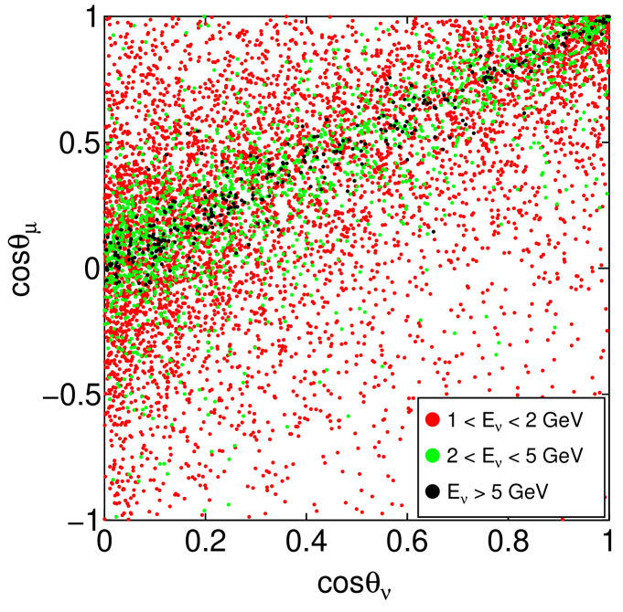
Figure 11: Correlation diagram between $\cos{\theta}_{\nu}$ and $\cos{\theta}_{\mu}$ for different neutrino energy regions.

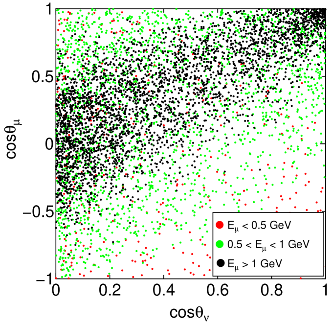
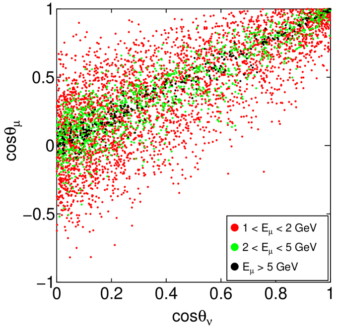
Figure 12: Correlation diagrams between ${\cos\theta_{\nu}}$ and $\cos{\theta}_{\mu}$ for different muon energy ranges.

Thus, it could be surely concluded from Fig. 11 and Fig. 12 that the SK assumption on the direction does not hold as a good estimator for the determination of the directions of the incident neutrinos even if statistically.

Finally, we examine the relation between the zenith angle distribution for upward $\nu_{\mu}$ and $\bar{\nu}_{\mu}$ and the corresponding zenith angle distribution for $\mu$ and $\bar{\mu}$ in the case of no oscillation. By perfoming the procedure described in Appendix C, we obtain a pair of ($\cos{\theta_{\mu}}$, $E_{\mu}$) from a sampling of ($\cos{\theta_{\nu}}$, $E_{\nu}$). In Figure 13, we show the relation between the upward incident neutrino zenith angle distribution and the emitted muon ones thus obtained for the null oscillation. If we guarantee the SK assumption on the direction, the emitted muon zenith angle distribution is expressed approximately as the incident neutrino zenith angle distribution. However, the really simulated muon zenith angle distribution is quite different from the incident neutrino zenith angle distribution. This is the reason why the SK assumption on the direction does not hold even if statistically. Furthermore, it should be noticed from the figure that the existence of the downward muons from the upward neutrinos could not be neglected which is enhanced by the azimuthal angles in addition to the backscattering. If the neutrino oscillation does not exist, such downward muons do not bring about problems, because in this case the zenith angle distribution of the downward neutrino is symmetrical to that of upward neutrino. Then, the ”inverted leptons” cancel out totally. However, in the case of the presence of the neutrino oscillation, such cancellation does not occur. Namely, the determination of the direction of the incident neutrinos estimated by the emitted muon should be more carefully treated.

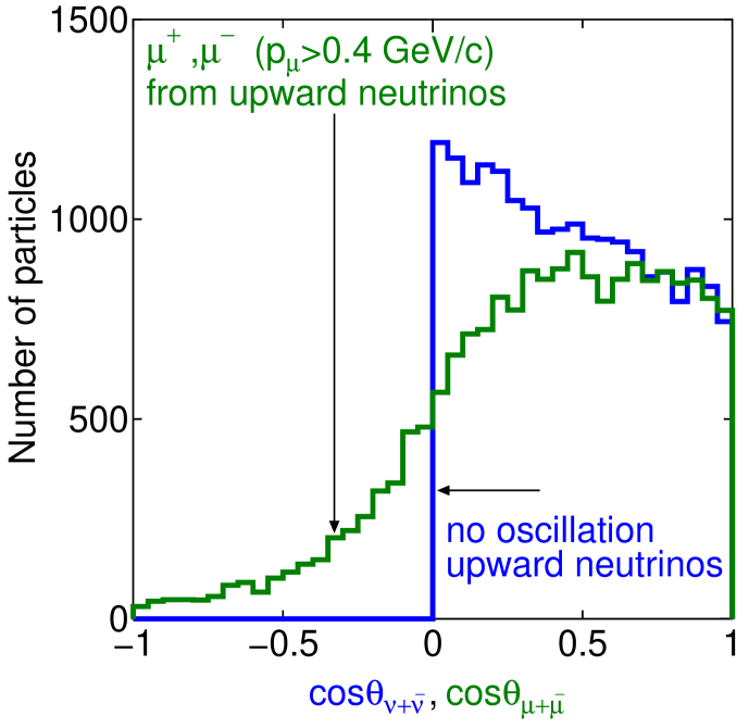
Figure 13: The relation between the zenith angle distribution of the incident neutrino and corresponding ones of the emitted lepton

6 Conclusions

We have shown the invalidity of the SK assumption on the direction for the analysis of the Single Ring $\mu$ Events among Fully Contained Events which are solid and free from the interpretation on their interaction types. Super-Kamiokande Collaboration have examined all possible neutrino events for the neutrino oscillation problem, say, Sub-GeV e-like Events, Multi-GeV e-like Events, Sub-GeV $\mu$-like Events, Multi-GeV $\mu$-like Events, multi-ring Sub GeV $\mu$-like Events, multi-ring Multi-GeV Events, PC Events, Upward Stopping Muon Events and Upward Through Going Muon Events (see, [12]), and all possible neutrino events provide the same neutrino oscillation parameters with the same precision accidentally. However, different types of neutrino events have different structures which are accompanied by different experimental uncertainties. Therefore, we could not readily believe such unified conclusions, taking into consideration the different experimental qualities in the different types of events. The most clear cut events among the SK events are one ring electron like events and muon-like events among Fully Contained Events. In these events, apart from the numerical uncertainties, one could essentially discriminate electron from muon (see footnote 1), and we decide the directions of the leptons as well as their energies, because we know the interaction points as well as their end points in the detector. Therefore, it is more desirable that one analyze the single-ring electron-like events and single-ring muon-like events among Fully Contained Events exclusively not being tempted by the increase of statistics. If one really finds the solid evidence for the neutrino oscillation in the most clear cut events, such as Single Ring $\mu$ Events, then one could find some corroboration for the neutrino oscillation even in the worst quality of experimental data, such as Upward Stopping Muon Events and Upward Through Going Muon Events.

In the subsequent paper (Part 2), we apply our present result to the analysis of the $L/E$ distribution for Single Ring $\mu$ Events due to QEL among Fully Contained Events which may lead the direct observation of the neutrino oscillation, if really exists, due to the simplicity of the events concerned. Also, we are now under preparation the third paper (Part 3) in which we examine the zenith angle distribution for the same type of the events mentioned above.

In the following Appendices we give the concrete Monte Carlo Simulations, namely, the details of our Time Sequential Simulation.

Appendix A Appendix: Monte Carlo Procedure for the Decision of Emitted Energies of the Leptons and Their Direction Cosines

Here, we give the Monte Carlo Simulation procedure for obtaining the energy and its direction cosines, $(l_{r},m_{r},n_{r})$, of the emitted lepton in QEL for a given energy and its direction cosines, $(l,m,n)$, of the incident neutrino.

The relation among $Q^{2}$, $E_{\nu+\bar{\nu}}$, the energy of the incident neutrino, $E_{\ell}$, the energy of the emitted lepton (muon or electron or their anti-particles) and $\theta_{\rm s}$, the scattering angle of the emitted lepton, is given as

$$Q^{2}=2E_{\nu(\bar{\nu})}E_{\ell(\bar{\ell})}(1-{\rm cos}\theta_{\rm s}).$$ (A·1)

Also, the energy of the emitted lepton is given by

$$E_{\ell(\bar{\ell})}=E_{\nu(\bar{\nu})}-\frac{Q^{2}}{2M}.$$ (A·2)

Procedure 1
We decide $Q^{2}$ from the probability function for the differential cross section with a given $E_{\nu(\bar{\nu})}$ (Eq. (2) in the text) by using the uniform random number, ${\xi}$, between (0,1) in the following

$$\xi=\int_{Q_{\rm min}^{2}}^{Q^{2}}P_{\ell(\bar{\ell})}(E_{\nu(\bar{\nu})},Q^{2}){\rm d}Q^{2},$$ (A·3)

where

$$P_{\ell(\bar{\ell})}(E_{\nu(\bar{\nu})},Q^{2})=$$

$$\frac{{\rm d}\sigma_{\ell(\bar{\ell})}(E_{\nu(\bar{\nu})},Q^{2})}{{\rm d}Q^{2}}\Bigg{/}\!\!\!\!\int_{Q_{\rm min}^{2}}^{Q_{\rm max}^{2}}\frac{{\rm d}\sigma_{\ell(\bar{\ell})}(E_{\nu(\bar{\nu})},Q^{2})}{{\rm d}Q^{2}}{\rm d}Q^{2}.$$

From Eq. (A$\cdot$1), we obtain $Q^{2}$ in histograms together with the corresponding theoretical curve in Fig. 14. The agreement between the sampling data and the theoretical curve is excellent, which shows the validity of the utlized procedure in Eq. (A $\cdot$3) is right.

Procedure 2
We obtain $E_{\ell(\bar{\ell})}$ from Eq. (A$\cdot$2) for the given $E_{\nu(\bar{\nu})}$ and $Q^{2}$ thus decided in the Procedure 1.

Procedure 3
We obtain $\cos{\theta_{\rm s}}$, cosine of the the scattering angle of the emitted lepton, for $E_{\ell(\bar{\ell})}$ thus decided in the Procedure 2 from Eq. (A$\cdot$1) .

Procedure 4
We decide $\phi$, the azimuthal angle of the scattering lepton, which is obtained from

$$\phi=2\pi\xi.$$ (A·5)

Here, $\xi$ is a uniform random number of the range (0, 1).
As explained schematically in the text(see Fig. 3 in the text), we must take account of the effect due to the azimuthal angle $\phi$ in the QEL to obtain the zenith angle distribution of both Fully Contained Events and Partially Contained Events correctly.

Procedure 5
The relation between direction cosines of the incident neutrinos, $(\ell_{\nu(\bar{\nu})},m_{\nu(\bar{\nu})},n_{\nu(\bar{\nu})})$, and those of the corresponding emitted lepton, $(\ell_{\rm r},m_{\rm r},n_{\rm r})$, for a certain $\theta_{\rm s}$ and $\phi$ is given as

$$\left(\begin{array}[]{c}\ell_{\rm r}\\ m_{\rm r}\\ n_{\rm r}\end{array}\right)=\left(\begin{array}[]{ccc}\displaystyle\frac{\ell n}{\sqrt{\ell^{2}+m^{2}}}&-\displaystyle\frac{m}{\sqrt{\ell^{2}+m^{2}}}&\ell_{\nu(\bar{\nu})}\\ \displaystyle\frac{mn}{\sqrt{\ell^{2}+m^{2}}}&\displaystyle\frac{\ell}{\sqrt{\ell^{2}+m^{2}}}&m_{\nu(\bar{\nu})}\\ -\sqrt{\ell^{2}+m^{2}}&0&n_{\nu(\bar{\nu})}\end{array}\right)\left(\begin{array}[]{c}{\rm sin}\theta_{\rm s}{\rm cos}\phi\\ {\rm sin}\theta_{\rm s}{\rm sin}\phi\\ {\rm cos}\theta_{\rm s},\end{array}\right),$$ (A·6)

where $n_{\nu(\bar{\nu})}={\rm cos}\theta_{\nu(\bar{\nu})}$, and $n_{\rm r}={\rm cos}\theta_{\ell}$. Here, $\theta_{\ell}$ is the zenith angle of the emitted lepton.

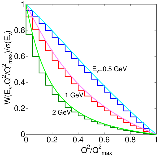
Figure 14: The reappearance of the probability function for QEL cross section. Histograms are sampling results, while the curves concerned are theoretical ones for given incident energies.

The Monte Carlo procedure for the determination of $\theta_{\ell}$ of the emitted lepton for the parent (anti-)neutrino with given $\theta_{\nu(\bar{\nu})}$ and $E_{\nu(\bar{\nu})}$ involves the following steps:

We obtain $(\ell_{r},m_{r},n_{r})$ by using Eq. (A·6). The $n_{r}$ is the cosine of the zenith angle of the emitted lepton which should be contrasted to $n_{\nu}$, that of the incident neutrino.
Repeating the procedures 1 to 5 just mentioned above, we obtain the zenith angle distribution of the emitted leptons for a given zenth angle of the incident neutrino with a definite energy.

In the SK analysis, instead of Eq. (A·6), they assume
$n_{r}=n_{\nu(\bar{\nu})}$ uniquely for ${E_{\mu(\bar{\mu})}}\geq$ 400 MeV.

Appendix B Appendix: Monte Carlo Procedure to Obtain the Zenith Angle of the Emitted Lepton for a Given Zentith Angle of the Incident Neutrino

The present simulation procedure for a given zenith angle of the incident neutrino starts from the atmospheric neutrino spectrum at the opposite site of the Earth to the SK detector. We define, $N_{\rm int}(E_{\nu(\bar{\nu})},t,{\rm cos}\theta_{\nu(\bar{\nu})})$, the interaction neutrino spectrum at the depth $t$ from the SK detector in the following way

$$N_{\rm int}(E_{\nu(\bar{\nu})},t,{\cos}\theta_{\nu(\bar{\nu})})=N_{\rm sp}(E_{\nu(\bar{\nu})},\cos\theta_{\nu(\bar{\nu})})\times$$

$$\Bigg{(}1-\frac{{\rm d}t}{\lambda_{1}(E_{\nu(\bar{\nu})},t_{1},\rho_{1})}\Bigg{)}\times\cdots\times\Bigg{(}1-\frac{{\rm d}t}{\lambda_{n}(E_{\nu(\bar{\nu})},t_{n},\rho_{n})}\Bigg{)}.$$

Here, $N_{\rm sp}(E_{\nu(\bar{\nu})},\cos\theta_{\nu(\bar{\nu})})$ is the atmospheric (anti-) neutrino spectrum for the zenith angle at the opposite surface of the Earth.

Here $\lambda_{i}(E_{\nu(\bar{\nu})},t_{i},\rho_{i})$ denotes the mean free path of the neutrino (anti neutrino) with the energy $E_{\nu(\bar{\nu})}$ due to QEL at the distance, $t_{i}$, from the opposite surface of the Earth inside whose density is $\rho_{i}$.

The procedures of the Monte Carlo Simulation for the incident neutrino(anti neutrino) with a given energy, $E_{\nu(\bar{\nu})}$, whose incident direction is expressde by $(l,m,n)$ are as follows.

Procedure A
For the given zenith angle of the incident neutrino, ${\theta_{\nu(\bar{\nu})}}$, we formulate, $N_{\rm pro}(E_{\nu(\bar{\nu})},t,\cos\theta_{\nu(\bar{\nu})}){\rm d}E_{\nu(\bar{\nu})}$ , the production function for the neutrino flux to produce leptons at the Kamioka site in the following

$$N_{\rm pro}(E_{\nu(\bar{\nu})},t,\cos\theta_{\nu(\bar{\nu})}){\rm d}E_{\nu(\bar{\nu})}$$ (B·2)

$$=\sigma_{\ell(\bar{\ell})}(E_{\nu(\bar{\nu})})N_{\rm int}(E_{\nu(\bar{\nu})},t,{\rm cos}\theta_{\nu(\bar{\nu})}){\rm d}E_{\nu(\bar{\nu})},$$

where

$$\sigma_{\ell(\bar{\ell})}(E_{\nu(\bar{\nu})})=\int^{Q_{\rm max}^{2}}_{Q_{\rm min}^{2}}\frac{{\rm d}\sigma_{\ell(\bar{\ell})}(E_{\nu(\bar{\nu})},Q^{2})}{{\rm d}Q^{2}}{\rm d}Q^{2}.$$ (B·3)

Each differential cross section above is given in Eq. (2) in the text.
Utilizing, $\xi$, the uniform random number between (0,1), we determine $E_{\nu(\bar{\nu})}$, the energy of the incident neutrino in the following sampling procedure

$$\xi=\int_{E_{\nu(\bar{\nu}),{\rm min}}}^{E_{\nu(\bar{\nu})}}P_{d}(E_{\nu(\bar{\nu})},t,\cos\theta_{\nu(\bar{\nu})}){\rm d}E_{\nu(\bar{\nu})},$$ (B·4)

where

$$P_{d}(E_{\nu(\bar{\nu})},t,\cos{\theta}_{\nu(\bar{\nu})}){\rm d}E_{\nu(\bar{\nu})}$$ (B·5)

$$= \frac{N_{pro}(E_{\nu(\bar{\nu})},t,\cos{\theta}_{\nu(\bar{\nu})}){\rm d}E_{\nu(\bar{\nu})}}{\displaystyle\int_{E_{\nu(\bar{\nu}),{\rm min}}}^{E_{\nu(\bar{\nu}),{\rm max}}}N_{pro}(E_{\nu(\bar{\nu})},t,\cos{\theta}_{\nu(\bar{\nu})}){\rm d}E_{\nu(\bar{\nu})}}.$$

In our Monte Carlo procedure,
the reproduction of, $P_{d}(E_{\nu(\bar{\nu})},t,\cos\theta_{\nu(\bar{\nu})}){\rm d}E_{\nu(\bar{\nu})}$, the normalized differential neutrino interaction probability function, is confirmed in the same way as in Eq. (A$\cdot$4).

Procedure B
For the (anti-)neutrino concerned with the energy of $E_{\nu(\bar{\nu})}$, we sample $Q^{2}$ utlizing $\xi_{3}$, the uniform random number between (0,1). The Procedure B is exactly the same as in the Procedure 1 in the Appendix A.

Procedure C
We decide, ${\theta_{\rm s}}$, the scattering angle of the emitted lepton for given $E_{\nu(\bar{\nu})}$ and $Q^{2}$. The procedure C is exactly the same as in the combination of Procedures 2 and 3 in the Appendix A.

Procedure D
We randomly sample the azimuthal angle of the charged lepton concerned. The Procedure D is exactly the same as in the Procedure 4 in the Appendix A.

Procedure E
We decide the direction cosine of the charged lepton concerned. The Procedure E is exactly the same as in the Procedure 5 in the Appendix A.

We repeat Procedures A to E until we reach the desired trial number.

Appendix C Appendix: Correlation between the Zenith Angles of the Incident Neutrinos and Those of the Emitted Leptons

Procedure A
By using, $N_{\rm pro}(E_{\nu(\bar{\nu})},t,\cos\theta_{\nu(\bar{\nu})}){\rm d}E_{\nu(\bar{\nu})}$, which is defined in Eq. (B·2),

we define the spectrum for $\cos\theta_{\nu(\bar{\nu})}$ in the following.

$$I(\cos\theta_{\nu(\bar{\nu})}){\rm d}(\cos\theta_{\nu(\bar{\nu})})=$$ (C·1)

$${\rm d}(\cos\theta_{\nu(\bar{\nu})})\int_{E_{\nu(\bar{\nu}),{\rm min}}}^{E_{\nu(\bar{\nu}),{\rm max}}}\!\!\!\!\!\!\!\!\!\!\!\!\!\!\!\!N_{\rm pro}(E_{\nu(\bar{\nu})},t,\cos\theta_{\nu(\bar{\nu})}){\rm d}E_{\nu(\bar{\nu})}.$$

By using Eq. (C·2) and $\xi$, a sampled uniform random number between (0,1), then we could determine $\cos\theta_{\nu(\bar{\nu})}$ from the following equation

$$\xi=\int_{0}^{\cos\theta_{\nu(\bar{\nu})}}P_{n}(\cos\theta_{\nu(\bar{\nu})}){\rm d}(\cos\theta_{\nu(\bar{\nu})}),$$ (C·2)

where

$$P_{n}(\cos\theta_{\nu(\bar{\nu})})=I(\cos\theta_{\nu(\bar{\nu})})\Bigg{/}\int_{0}^{1}I(\cos\theta_{\nu(\bar{\nu})}){\rm d}(\cos\theta_{\nu(\bar{\nu})}).$$ (C·3)

Procedure B
For the sampled ${\rm d}(\cos\theta_{\nu(\bar{\nu})})$ in the Procedure A, we sample $E_{\nu(\bar{\nu})}$ from Eq.(C·4) by using ${\xi}$, the uniform randum number between (0,1)

$$\xi=\int_{E_{\nu(\bar{\nu}),{\rm min}}}^{E_{\nu(\bar{\nu})}}P_{pro}(E_{\nu(\bar{\nu})},\cos\theta_{\nu(\bar{\nu})}){\rm d}E_{\nu(\bar{\nu})},$$ (C·4)

where

$$P_{pro}(E_{\nu(\bar{\nu})},t,\cos\theta_{\nu(\bar{\nu})}){\rm d}E_{\nu(\bar{\nu})}=$$ (C·5)

$$\frac{N_{\rm pro}(E_{\nu(\bar{\nu})},t,\cos\theta_{\nu(\bar{\nu})}){\rm d}E_{\nu(\bar{\nu})}}{\displaystyle\int_{E_{\nu(\bar{\nu}),{\rm min}}}^{E_{\nu(\bar{\nu}),{\rm max}}}N_{\rm pro}(E_{\nu(\bar{\nu})},t,\cos\theta_{\nu(\bar{\nu})}){\rm d}E_{\nu(\bar{\nu})}}.$$

Procedure C
For the sampled $E_{\nu(\bar{\nu})}$ in the Procedure B, we sample $E_{\mu(\bar{\mu})}$ from Eqs. (A·2) and (A·3). For the sampled $E_{\nu(\bar{\nu})}$ and $E_{\mu(\bar{\mu})}$, we determine $\cos{\theta}_{s}$, the scattering angle of the muon uniquely from Eq. (A·1).

Procedure D
We determine, $\phi$, the azimuthal angle of the scattering lepton from Eq. (A·5) by using ${\xi}$, an uniform randum number between (0,1).

Procedure E
We obtain $\cos{\theta}_{\mu(\bar{\mu})}$ from Eq. (A·6). As the result, we obtain a pair of ($\cos\theta_{\nu(\bar{\nu})}$, $\cos{\theta}_{\mu(\bar{\mu})}$) through Procedures A to E. Repeating the Procedures A to E, we finally the correlation between the zenith angle of the incident neutrino and that of the emitted muon.

References

References

-
[1]
Hirata, KS et al., Phys.Lett.B205(1988)416
Hirata, KS et al., Phys.Lett.B280(1992)146
Casper, D et al., Phys.Rev.Lett.66(1991)2561
Becker-Szendy, R et al., Phys.Rev. D 46(1992)3720. - [2] Hatakeyama, S et al., Phys.Rev.Lett.81(1998)2010.
-
[3]
Kajita, T, Neutrino 98, Takayama, Japan, June 4-9 1998
Fukuda, Y, Phys.Rev.Lett.81(1998)1562. -
[4]
Mann, WA, Nucl.Phys.Proc.Supple Vol.91(2000)134
Ambrosio, Met al., Phys.Lett.B478(2000)3. - [5] K2K, Phys.Rev. D74(2006)72003
- [6] Michael, DG et al., Phys.Rev.Lett.97(2006) 191801
- [7] Kajita, T and Totsuka, Y, Rev. Mod. Phys., 73 (2001) 85. See p. 101.
- [8] Ishitsuka, M, Ph.D thesis, University of Tokyo (2004). See p. 138.
- [9] Jung, CK, Kajita, T, Mann, T and McGrew, C, Anual. Rev. Mod. Sci. vol.15 (2005) 431
- [10] Renton, P., Electro-weak Interaction, Cambridge University Press (1990). See p. 405.
- [11] Honda, M., et al., Phys. Rev. D 52 (1996) 4985
- [12] Ashie,Y. et al., Phys. Rev. D 71 (2005) 112005.