Bipartite Units of Nonlocality

Abstract

Imagine a task in which a group of separated players aim to simulate a statistic that violates a Bell inequality. Given measurement choices the players shall announce an output based solely on the results of local operations – which they can discuss before the separation – on shared random data and shared copies of a so-called unit correlation. In the first part of this article we show that in such a setting the simulation of any bipartite correlation, not containing the possibility of signaling, can be made arbitrarily accurate by increasing the number of shared Popescu-Rohrlich (PR) boxes. This establishes the PR box as a simple asymptotic unit of bipartite nonlocality. In the second part we study whether this property extends to the multipartite case. More generally, we ask if it is possible for separated players to asymptotically reproduce any nonsignaling statistic by local operations on bipartite unit correlations. We find that non-adaptive strategies are limited by a constant accuracy and that arbitrary strategies on $n$ resource correlations make a mistake with a probability greater or equal to $c/n$, for some constant $c$.

I Introduction

The correlation in the outputs of certain quantum experiments on pairs of separated particles cannot be explained by information shared before the separation. This property is called quantum nonlocality and manifests itself in the violation of Bell inequalities Bell (1964); Clauser et al. (1969). Nonlocal quantum correlations have opened new opportunities for information processing such as, for example, quantum key distribution Barrett et al. (2005); Acín et al. (2007); Masanes (2009); Hänggi et al. (2010) with device-independent secrecy. Correlations that do not offer the possibility of signaling can be represented, when measurement and outcome dimensions are fixed, by so-called nonsignaling polytopes of which quantum correlations are a proper subset Tsirelson (1980). Some elements in these convex sets are more useful for distributed tasks than others van Dam (2005); Linden et al. (2007); Brassard et al. (2006); Brunner and Skrzypczyk (2009). Thus, a number of theoretical questions on the relationship and possible reductions between different nonsignaling correlations have emerged. In the context of quantum correlations the singlet state has been established as a unit of entanglement: A supply of singlets can be transformed into any other bipartite pure state by local operations and classical communication, and vice versa Bennett et al. (1996). This reversibility partly relies on asymptotic transformations and does not hold in general, that is, for multipartite states or bipartite mixed states. Summing up, we have that any entangled state can be approximated from sufficiently many copies of the singlet state.

An analogous question when the objects are not quantum states, but general nonlocal correlations, motivates the search for a unit of nonlocality. More specifically, the identification of a nontrivial set of correlations from which any other nonsignaling statistic can be derived, is intended Barrett et al. (2005); Jones and Masanes (2005); Barrett and Pironio (2005); Dupuis et al. (2007). The following game illustrates the problem: In the initial phase a group of players is given a description of certain input-output correlations. They are allowed to discuss a strategy but are then separated in order to prevent them from communicating. Now the test phase begins. Each player is given a secret input and announces an output. This is repeated many times independently. The objective of the players is to minimize the distance of their input-output distribution from the described target correlations.

Any local correlation can be simulated perfectly by the players if they share the right classical information before they get separated. However, the game becomes more challenging if the described correlation is nonlocal, that is, if it violates a Bell inequality. In this case any simulation must be faulty Bell (1964). It is then natural to ask which minimal set of nonlocal resources the players additionally require to win the game. If such a set allows for simulating any nonsignaling correlation, it can be considered a unit of nonlocality. The Popescu-Rohrlich box Khalfin and Tsirelson (1985); Popescu and Rohrlich (1994) (PR box) has been shown to be a unit for bipartite correlations restricted to binary outputs Jones and Masanes (2005); Barrett and Pironio (2005) and, in the converse situation, for bipartite correlations restricted to binary inputs Barrett et al. (2005). In the latter case the simulation can be made arbitrary close but not perfect. The existence of a bipartite unit that allows the zero-error simulation of any target correlation, has been ruled out by counter examples in the multipartite case Barrett and Pironio (2005) and later also for bipartite target correlations Dupuis et al. (2007).

However, the study of a unit of nonlocality is based on the analogous result in entanglement theory that establishes the singlet as a unit of entanglement. Some of these transformations are not error-free but rather approximations that can be made arbitrarily close. It is clear that in the described simulation game, as well as in real-world experiments, a sufficiently small simulation error can be hidden from the tester. Furthermore, in the context of information processing tasks, asymptotic reductions between different nonlocal resources are often satisfying. It is therefore both natural and meaningful to establish a unit that allows for asymptotically perfect simulations.

This is the aim of the present article. The PR box, as suggested by various contributions, is confirmed to have the properties of an asymptotic unit of bipartite nonlocality. We will describe a hierarchy of simulation protocols that allows two players to transform a finite supply of PR boxes into an arbitrarily close approximation to any desired bipartite correlation (Theorem 1). Furthermore, we will analyze the simulation’s performance in terms of resource consumption (Theorem 2). Then, the theoretical possibility of bipartite units for the multipartite case is studied. We demonstrate two limitations. Inspired by Barrett and Pironio (2005), we construct an instance of a multipartite simulation game that can provably not be won arbitrarily often with non-adaptive protocols even when the players have access to any set of bipartite nonsignaling resources (Corollary 1). Also, we will show that if the players are allowed to execute any non-interactive protocol, then the simulation error of the same game instance is connected with the balance of the players output functions. As a consequence we calculate a linear rate at which the simulation distance maximally declines when increasing the number of shared resource correlations (Theorem 4).

II Preliminaries

Adopting the abstracted approach to nonlocality formulated by generalized nonsignaling theories Barrett et al. (2005), we consider correlations in the joint behavior of the ends of an input-output system. An $m$-partite system is characterized by joint probability distributions $P_{A}^{x}$ on $m$ random variables $A=(A_{1},\ldots,A_{m})$ that map to the value space $\mathcal{A}_{1}\times\dots\times\mathcal{A}_{m}$, representing the outputs of the system, conditioned on $m$ inputs $x=(x_{1},\ldots,x_{m})\in\mathcal{X}_{1}\times\dots\times\mathcal{X}_{m}$. See Figure 1.

Figure 1: Schematic representation of the ends of an $m$-partite system. The system outputs $a=(a_{1},a_{2},\ldots,a_{m})$ on inputs $x=(x_{1},x_{2},\ldots,x_{m})$ with probability $P_{A}^{x}(a)$.

Furthermore, $P_{A}^{x}$ is nonsignaling, meaning that for any subset $S\subseteq[m]$ – we use $[m]$ for short to denote the set $\{1,\ldots,m\}$ – the marginal distribution $P_{A_{S}}^{x_{S},x_{\bar{S}}}$ is independent of the inputs $x_{\bar{S}}=\{x_{i}:i\in[m]\backslash S\}$.

Now, consider the following task: In a first phase, a group of $m$ players is given a description of a system $T$, called the target system. Furthermore, the players can share classical information, such as a global value $\lambda$ from some distribution $P_{\Lambda}$, and choose any collection of resource systems from some predefined set. After discussing a strategy and sharing the resource systems among each other, they are separated in order to prevent any communication. Then the test phase begins. The players are given inputs $x=(x_{1},\ldots,x_{m})$, such that each one of them learns only its own input and has no information on the other inputs. Then each player determines an output $a_{i}$ resulting in an overall output string $a=(a_{1},\ldots,a_{m})$, such that, after an arbitrary number of independent rounds, the simulated system $S$ is as close as possible to $T$. This means they aim at minimizing the following measure.

Definition 1 (simulation distance).

A simulated system $S$ approximates a target system $T$ with distance

$$\delta(S,T)=\max_{x}\frac{1}{2}\sum_{a}|S_{A}^{x}(a)-T_{A}^{x}(a)|.$$

For fixed inputs $x$ the outputs of the simulated system and the outputs of the target system are distributed according to $S_{A}^{x}$ and $T_{A}^{x}$, respectively. The distance between the two distributions can be quantified by their total variation distance $1/2\sum_{a}|S_{A}^{x}(a)-T_{A}^{x}(a)|$. Informally speaking, the simulation distance $\delta(S,T)$ expresses the worst total variation distance that a tester may reveal between the simulated system and the target system.

The strategy on which the players agree is called a simulation protocol. It typically includes a plan of which classical distribution and which resource systems are shared and how they are used by each one of them to help in the simulation. The players can apply any classical circuitry to their local parts of the shared systems. Such a local input-output strategy is called a wiring  Barrett et al. (2005); Short et al. (2006). Note that when interacting with a system one receives an output immediately after providing an input, independently of whether the player in possession of the other end has given its input already. This is an allowed convention because all systems satisfy the nonsignaling constraints.

II.1 Simulation protocols

Given inputs $x_{1},\ldots,x_{m}$ and a global random value $\lambda$, which is drawn from the distribution $P_{\Lambda}$, the players execute their local protocols on the shared resource systems and determine a final output. We identify two classes of simulation protocols by distinguishing the players’ local strategies.

The first class allows each player’s wiring to consist of arbitrary local, classical operations on the inputs and outputs of the shared resource systems. This is the most general description of a simulation protocol, which we shall call adaptive. Suppose that player $i\in[m]$ shares the $n$ resource systems $R_{1},\ldots,R_{n}$ with other players. In an adaptive simulation protocol, given an input $x_{i}$ and the shared random value $\lambda$, player $i$’s possibilities consist of the following parts.

1. Player $i$ inputs $f_{1}(x_{i},\lambda)$ to the shared system $R_{i_{1}}$, where the index $i_{1}$ is determined by the function $i_{1}(x_{i},\lambda)$. System $R_{i_{1}}$ outputs $b_{i_{1}}$ to player $i$.

2. Player $i$ then inputs $f_{2}(x_{i},\lambda,b_{i_{1}})$ to $R_{i_{2}}$, where the index of the second system to use is determined by the local function $i_{2}=i_{2}(x_{i},\lambda,b_{i_{1}})$, obtaining the output $b_{i_{2}}$.

   $\vdots$

3. Player $i$ continues doing so until all $n$ systems have provided an output. In the end the local variables $b=(b_{1},\ldots,b_{n})$ are completely assigned. The final output of player $i$ is then given by the result of the local function $f^{x_{i}}(\lambda,b)$.

Locally, an adaptive simulation protocol may consist of as many as $n$ dependent blocks of classical operations, or rounds, generating inputs to and obtaining outputs from the shared systems.

The second class imposes the natural restriction of parallelism to the set of adaptive protocols. Each player is limited to execute a single block of classical operations. Thus, this class includes only those protocols in which each player determines the inputs into all shared resource systems solely from its initial input and $\lambda$. In these so-called non-adaptive simulation protocols the wiring for player $i$ is such that no input into a resource system depends on the output of another, and there is no order in using the systems – all ends can be evaluated in parallel, immediately after having learned $x_{i}$ and $\lambda$. Therefore, any wiring of a non-adaptive protocol can be described by the input functions $f_{1}(x_{i},\lambda),\ldots,f_{n}(x_{i},\lambda)$ and the final output function $f^{x_{i}}(\lambda,b)$.

In both classes, each player has the freedom to define its own collection of local functions and, therefore, an individual wiring of the described kind.

II.2 Classes of systems

Typically, an instance of the simulation game is challenging if the set of resource systems the players are allowed to use, is restricted and the target correlation is nonlocal. We will define a set of multipartite target systems and a set of bipartite resource systems for which the simulation game is particularly difficult.

The following system is inspired by a GHZ quantum correlation (after the authors of Greenberger et al. (1989), Greenberger, Horne, and Zeilinger) exhibiting quantum nonlocality DiVincenzo and Peres (1997). See also Barrett and Pironio (2005), which introduces this target system in the present context of simulation games.

Example 1.

Let $T$ be any five-partite system with binary inputs $\mathcal{X}_{1},\ldots,\mathcal{X}_{5}=\{0,1\}$ and binary outputs $\mathcal{A}_{1},\ldots,\mathcal{A}_{5}=\{0,1\}$, fulfilling the following six correlation conditions:

$$\text{If }x_{1}=0,x_{2}=1 ,x_{3}=0,$$

$$\text{then }a_{1}+a_{2}+a_{3}\equiv 0~{}({\text{\em mod }}2).$$ (1)

$$\text{If }x_{2}=0,x_{3}=1 ,x_{4}=0,$$

$$\text{then }a_{2}+a_{3}+a_{4}\equiv 0~{}({\text{\em mod }}2).$$ (2)

$$\text{If }x_{3}=0,x_{4}=1 ,x_{5}=0,$$

$$\text{then }a_{3}+a_{4}+a_{5}\equiv 0~{}({\text{\em mod }}2).$$ (3)

$$\text{If }x_{4}=0,x_{5}=1 ,x_{1}=0,$$

$$\text{then }a_{4}+a_{5}+a_{1}\equiv 0~{}({\text{\em mod }}2).$$ (4)

$$\text{If }x_{5}=0,x_{1}=1 ,x_{2}=0,$$

$$\text{then }a_{5}+a_{1}+a_{2}\equiv 0~{}({\text{\em mod }}2).$$ (5)

$$\text{If }x_{1}=x_{2}=x_{3}~{} =x_{4}=x_{5}=1,$$

$$\text{then }a_{1}+ ~{}a_{2}+a_{3}+a_{4}+a_{5}\equiv 1~{}({\text{\em mod }}2).$$ (6)

For measurements on the corresponding quantum state, we additionally have that all output bits, and the parity of all subsets of output bits, that are not specified above, are uniformly random.

Let $\mathcal{P}^{b}$ stand for the set of all systems with $m=2$, henceforth called bipartite systems. The following class of bipartite resource systems essentially calculates any decision problem distributed between two parties.

Definition 2.

Let the set $\mathcal{R}$ include all bipartite systems $R_{AB}^{xy}$ with binary output alphabets $\mathcal{A}=\mathcal{B}=\{0,1\}$, and the joint probability distributions

$$R_{AB}^{xy}(a,b)=\begin{cases}\tfrac{1}{2}&\text{ if }a+b\equiv g(x,y)~{}({\text{\em mod }}2),\\ 0&\text{ otherwise},\end{cases}$$

where $g:\mathcal{X}\times\mathcal{Y}\rightarrow\{0,1\}$ is an arbitrary Boolean function on the inputs.

The next special class of bipartite systems generalizes the class $\mathcal{R}$ to an arbitrary output alphabet size.

Definition 3.

Let the set $\mathcal{D}$ include all bipartite systems $D_{AB}^{xy}$ with output alphabets $\mathcal{A}=\mathcal{B}=[d]$, for any integer $d>1$, and the joint probability distributions

$$D_{AB}^{xy}(a,b)=\begin{cases}\tfrac{1}{d}&\text{if }f^{xy}(a)=b,\\ 0&\text{otherwise},\end{cases}$$

where $f^{xy}:[d]\rightarrow[d]$ are permutations on the output set indexed by the inputs $x,y$.

Every system $D\in\mathcal{D}$ can equivalently be described by input alphabets $\mathcal{X},\mathcal{Y}$, an integer $d>1$ and a set of permutations $\{f^{xy}:x\in\mathcal{X},y\in\mathcal{Y}\}$ on $[d]$.

It is easy to see that the marginal probabilities $D_{A}^{x}(a)$ as well as $D_{B}^{y}(b)$ are uniform, independently of $y$ and $x$, respectively. Therefore, $\mathcal{D}\subset\mathcal{P}^{b}$ holds. Obviously, we have the relationship $\mathcal{R}\subset\mathcal{D}$ with any system in $\mathcal{R}$ identified by $\mathcal{X},\mathcal{Y}$, the integer $d=2$ and the set of permutations $\{g(x,y)+a~{}(\text{mod }2):x\in\mathcal{X},y\in\mathcal{Y}\}$.

We refer to the PR box Khalfin and Tsirelson (1985); Popescu and Rohrlich (1994) as the most prominent element of $\mathcal{R}$. Its correlations can be described as follows: On inputs $x,y\in\{0,1\}$, the system returns outputs $a,b\in\{0,1\}$, such that $a$ and $b$ alone are uniform and independent of $(x,y)$, but the correlation $xy\equiv a+b~{}(\text{mod }2)$ always holds.

Definition 4.

The PR box is a bipartite system with binary output alphabets $\mathcal{X}=\mathcal{Y}=\{0,1\}$ and binary input alphabets $\mathcal{A}=\mathcal{B}=\{0,1\}$ and the joint probability distributions

$$P_{PR}^{xy}(a,b)=\begin{cases}\tfrac{1}{2}&\text{if }a+b\equiv xy~{}({\text{\em mod }}2),\\ 0&\text{otherwise}.\end{cases}$$

The PR box violates the Clauser-Horne-Shimony-Holt inequality Clauser et al. (1969) – a Bell inequality in minimal dimensions – to the algebraic maximum. It follows from a work of Tsirelson Tsirelson (1980) that the correlation of the PR box is super-quantum, that is, that it cannot be approximated arbitrarily well by two parties performing quantum mechanical experiments. However, it can be approximated with an accuracy of roughly $85\%$, whereas $75\%$ is the local limit.

Finally, we introduce a compact way to describe different simulation results.

Definition 5.

We denote the existence of simulation protocols approximating any target system of the set $\mathcal{T}$ with resource systems restricted to the set $\mathcal{R}$ by the notation $\mathcal{R}\leadsto^{\varepsilon}\mathcal{T}$ and the possibility of zero-error simulations by $\mathcal{R}\leadsto\mathcal{T}$.

We are now sufficiently equipped to start with the statements and proofs of this articles contributions.

III A unit of bipartite nonlocality

In this section, we consider the simulation game for any system in $\mathcal{P}^{b}$. Given the description of any bipartite system, we ask which minimal set of bipartite resource systems is required by two players to agree on a simulation strategy that imitates the specified target arbitrarily well. As the main result of this section, we will prove that a finite supply of copies of a PR box as a resource is sufficient for this task.

Van Dam van Dam (2005) has given a construction of arbitrary Boolean functions distributed between two parties, which coincide with our set $\mathcal{R}$, with shared PR boxes. We will use this result later. In an intermediate step, we prove the existence of simulation protocols approximating $\mathcal{D}$ with resources from $\mathcal{R}$ (Lemma 4). This insight will then be generalized by an explicit, asymptotic reduction of arbitrary bipartite nonsignaling systems to $\mathcal{D}$ (Lemma 5). The main result (Theorem 1) is a consequence of these three parts as illustrated by the following proof outline.

van Dam (2005)	Lemma 4	Lemma 5		Theorem 1
$P_{PR}\leadsto\mathcal{R}$	$\mathcal{R}\leadsto^{\varepsilon}\mathcal{D}$	$\mathcal{D}\leadsto^{\varepsilon}\mathcal{P}^{b}$	$\Rightarrow$	$P_{PR}\leadsto^{\varepsilon}\mathcal{P}^{b}$

III.1 Interconverting $\mathcal{R}$ and $\mathcal{D}$

As a first step we concentrate on the slightly simpler situation where the target system is from $\mathcal{D}$, and the resources must be elements of $\mathcal{R}$. The proof idea is as follows: We argue inductively, over the size of the output alphabets, by constructing a simulation protocol that approximates a system $D\in\mathcal{D}$, with output sets $\mathcal{A}=\mathcal{B}=[d]$, from shared randomness and a finite number of copies of a certain system $D^{\prime}(D)\in\mathcal{D}$ with $\mathcal{A}^{\prime}=\mathcal{B}^{\prime}=[d-1]$. Roughly speaking, our protocol uses appropriately chosen permutations on the smaller output set of the resource system $D^{\prime}(D)$ to approximate the permutation distributions of $D$. For $d=2$ we recover the resource set $\mathcal{R}$ and, therefore, $\mathcal{R}\leadsto^{\varepsilon}\mathcal{D}$ follows.

Suppose we are given the system $D\in\mathcal{D}$ with input sets $\mathcal{X}$ and $\mathcal{Y}$ and output alphabet $[d]$. Then, let the system $D^{\prime}(D)$ be defined by the set

$$\{f^{(x,\hat{a})(y,\hat{b})}:(x,\hat{a})\in\mathcal{X}\times[d],(y,\hat{b})\in\mathcal{Y}\times[d]\}$$

of functions. Each $f^{(x,\hat{a})(y,\hat{b})}:[d-1]\rightarrow[d-1]$ is constructed from the set of permutations defining $D$, that is from $\{f^{xy}:x\in\mathcal{X},y\in\mathcal{Y}\}$, by the following rule.

$$f^{(x,\hat{a})(y,\hat{b})}(a)=\left\{\begin{array}[]{ll}r_{\hat{b}}^{-1}(f^{xy}(\hat{a}))&\text{if }f^{xy}(a)=\hat{b},a\neq\hat{a},\\ r_{\hat{b}}^{-1}(f^{xy}(r_{\hat{a}}(a)))&\text{otherwise},\end{array}\right.$$ (9)

where $r_{\hat{a}}:[d-1]\rightarrow[d]\backslash\{\hat{a}\}$ and $r_{\hat{b}}:[d-1]\rightarrow[d]\backslash\{\hat{b}\}$ are the simple bijections

$$r_{\hat{a}}(a)=\left\{\begin{array}[]{ll}d&\text{if }a=\hat{a},\\ a&\text{otherwise},\end{array}\right.~{}~{}r_{\hat{b}}(b)=\left\{\begin{array}[]{ll}d&\text{if }b=\hat{b},\\ b&\text{otherwise}.\end{array}\right.$$ (14)

For any given $D\in\mathcal{D}$ this construction yields a new system $D^{\prime}(D)$ that depends on the permutations defining $D$ and has an output alphabet that lacks one element compared to $D$. As promised, we can show that $D^{\prime}(D)$ is also in $\mathcal{D}$.

Lemma 1.

If $D\in\mathcal{D}$, then $D^{\prime}(D)\in\mathcal{D}$.

Proof.

We will show that for all $(x,\hat{a})\in\mathcal{X}\times[d]$ and all $(y,\hat{b})\in\mathcal{Y}\times[d]$, the function $f^{(x,\hat{a})(y,\hat{b})}$ is a permutation on the set $[d-1]$. For all inputs $a\in[d-1]$ we have $r_{\hat{a}}(a)\neq\hat{a}$ by (14). Therefore, we need only to distinguish two cases from (9). First,

$$\forall a,a^{\prime}\in[d-1]:~{} f^{(x,\hat{a})(y,\hat{b})}(a)=f^{(x,\hat{a})(y,\hat{b})}(a^{\prime})$$

$$\Rightarrow r_{\hat{b}}^{-1}(f^{xy}(\hat{a}))=r_{\hat{b}}^{-1}(f^{xy}(\hat{a}))$$

$$\Rightarrow f^{xy}(a)=\hat{b},f^{xy}(a^{\prime})=\hat{b},$$

$$~{}~{}~{}~{}~{}~{}~{}~{}a\neq\hat{a},a^{\prime}\neq\hat{a}$$

$$\Rightarrow f^{xy}(a)=f^{xy}(a^{\prime})$$

$$\Rightarrow a=a^{\prime},$$

where we used that $D\in\mathcal{D}$ and, therefore, implicitly that for any $x,y$ the function $f^{xy}$ is a permutation. Second,

$$\forall a,a^{\prime}\in[d-1]:~{} f^{(x,\hat{a})(y,\hat{b})}(a)=f^{(x,\hat{a})(y,\hat{b})}(a^{\prime})$$

$$\Rightarrow r_{\hat{b}}^{-1}(f^{xy}(r_{\hat{a}}(a)))=r_{\hat{b}}^{-1}(f^{xy}(r_{\hat{a}}(a^{\prime})))$$

$$\Rightarrow a=a^{\prime},$$

since $r_{\hat{b}}^{-1}$ and $r_{\hat{a}}$ are defined as bijections and we have that $f^{xy}$ is a permutation. Thus, $f^{(x,\hat{a})(y,\hat{b})}$ is injective from a finite set to itself — a permutation on $[d-1]$.∎

Now we describe the classical, local operations on which two players, called Alice and Bob, can agree before they get separated and which will allow them to emulate any wanted $D\in\mathcal{D}$ from a finite supply of shared copies of the system $D^{\prime}(D)\in\mathcal{D}$ to an arbitrary simulation distance. The simulation protocol consists of a finite number of rounds. Each round includes four steps subsequently and locally executed by Alice and Bob.

1. The first step is different in the initial round than in subsequent rounds.

   In the initial round Alice draws the local value $\hat{a}\sim\mathcal{U}_{[d]}$ and Bob draws $\hat{b}\sim\mathcal{U}_{[d]}$, that is, uniformly at random from the set $[d]$.

   Otherwise, in any subsequent round of the simulation, Alice uses the already obtained local value $a_{t}\in[d]$ and Bob uses $b_{t}\in[d]$, respectively, to assign $\hat{a}=a_{t}$ and $\hat{b}=b_{t}$.

2. Alice and Bob obtain the shared random bit $\lambda$, such that $P_{\Lambda}(\lambda=0)=1/d$ and $\lambda=1$ otherwise.

3. The shared resource system $D^{\prime}$ gets inputs $(x,\hat{a})$ from Alice and $(y,\hat{b})$ from Bob and outputs $a\in[d-1]$ to Alice and $b\in[d-1]$ to Bob.

4. Alice and Bob then process the obtained local data to derive the values $a_{t}\in[d]$ and $b_{t}\in[d]$ as

   $$a_{t}=\begin{cases}\hat{a}&\text{if }\lambda=0,\\ r_{\hat{a}}(a)&\text{otherwise},\end{cases}~{}~{}b_{t}=\begin{cases}\hat{b}&\text{if }\lambda=0,\\ r_{\hat{b}}(b)&\text{otherwise}.\end{cases}$$

The next round of the protocol starts with the first step as described above and proceeds according to the second step and so on. Figure 3 illustrates a subsequent round. After the last round the parties output $a_{t}$ and $b_{t}$ as the final outputs of the simulation.

The relabeling functions $r_{\hat{a}}$, $r_{\hat{b}}$ are necessary because the set $[d-1]$, on which the permutation $f^{(x,\hat{a})(y,\hat{b})}$ is defined, obviously lacks the element $d$, which is one of $D$’s outputs. On the other hand, we have already correlated the outputs $\hat{a}$ and $\hat{b}$ in the case $\lambda=0$, so this pair of outputs can serve as a substitution for $d$ and $f^{xy}(d)$, respectively.

Figure 3 illustrates the protocol approximating a target system $D$ with $n$ rounds.

Figure 2: One round of the simulation protocol. On local data $x,a_{t}$ and $y,b_{t}$, Alice and Bob decide to use the outputs of $D^{\prime}$ on inputs $(x,\hat{a})$ and $(y,\hat{b})$ with a probability of $P_{\Lambda}(\lambda=1)$ and to continue with the original pair $\hat{a},\hat{b}$ otherwise.

Figure 3: The approximate simulation of $D$ by shared randomness and local operations on $n$ copies of the system $D^{\prime}(D)$.

Now we prove two lemmas that describe useful properties of the presented protocol. Given are inputs $x,y$. At the beginning of every round, Alice and Bob hold a pair $\hat{a},\hat{b}$. If $f^{xy}(\hat{a})\neq\hat{b}$, then we have a certain probability with which the simulation of $D$ fails in that round.

Lemma 2.

In a round initialized with $\hat{a}$ and $\hat{b}$, such that $f^{xy}(\hat{a})\neq\hat{b}$, Alice and Bob generate outputs $a_{t}$ and $b_{t}$ that do not agree with the required correlation in $D_{AB}^{xy}$ with probability $2/d$.

Proof.

After initializing $\hat{a}$ and $\hat{b}$ the second step of the simulation round follows. The possible events are:
If $\lambda=0$, where $P_{\Lambda}(0)=1/d$, then Alice and Bob assign $a_{t}=\hat{a},b_{t}=\hat{b}$, which is an incorrect correlation.
If $\lambda=1$, where $P_{\Lambda}(1)=(d-1)/d$, then Alice and Bob assign $a_{t}=r_{\hat{a}}(a)$, $b_{t}=r_{\hat{b}}(b)$. By (9), the definition of $f^{(x,\hat{a})(y,\hat{b})}$, we have that the output pair $a,b$ obtained from $D^{\prime}$ obeys the permutation $f^{(x,\hat{a})(y,\hat{b})}(a)=b$. In this case we must distinguish three possible situations:
(1) If Alice gets $a$ such that $f^{xy}(a)=\hat{b}$, which happens with a maximal probability of $1/(d-1)$, then an error occurs because, by the definition of $r_{\hat{a}}$, Alice will never output $\hat{a}$ if $\lambda=1$. The round then finishes with the pair

$$a_{t} =r_{\hat{a}}(a)=a,$$

$$b_{t} =r_{\hat{b}}(f^{(x,\hat{a})(y,\hat{b})}(a))=r_{\hat{b}}(r_{\hat{b}}^{-1}(f^{xy}(\hat{a})))=f^{xy}(\hat{a})\neq\hat{b}.$$

(2) If Alice gets $a=\hat{a}$, which can happen if $\hat{a}\neq d$, then the round finishes with the correctly correlated pair

$$a_{t} =r_{\hat{a}}(\hat{a})=d,$$

$$b_{t} =r_{\hat{b}}(f^{(x,\hat{a})(y,\hat{b})}(\hat{a}))=r_{\hat{b}}(r_{\hat{b}}^{-1}(f^{xy}(r_{\hat{a}}(\hat{a}))))=f^{xy}(d).$$

(3) If Alice gets any other $a\in[d-1]$, then the round finishes with the correctly correlated pair

$$a_{t} =r_{\hat{a}}(a)=a,$$

$$b_{t} =r_{\hat{b}}(f^{(x,\hat{a})(y,\hat{b})}(a))=r_{\hat{b}}(r_{\hat{b}}^{-1}(f^{xy}(r_{\hat{a}}(a))))=f^{xy}(a).$$

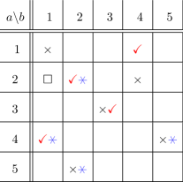
Figure 4: An illustration of Lemma 2: Suppose a round initialized with $\hat{a}=2$ and $\hat{b}=1$ such that $f^{xy}(\hat{a})\neq\hat{b}$ ($\square$). Such a permutation on the set $[d=5]$ is indicated with crosses ($\times$). The corresponding permutation $f^{(x,\hat{a})(y,\hat{b})}$ is shown with check-marks (✓). The relabelings $r_{\hat{a}=2}$ and $r_{\hat{b}=1}$ correlate $(5,2)$ by $(2,2)$ and $(4,5)$ by $(4,1)$ (indicated by $\hexstar$). Therefore, this round ends with an incorrect pair if $\lambda=0$ or if Alice gets $a=1$, which happens with a total chance $2/5$.

Therefore, the round will certainly end in a bad pair if $\lambda=0$. Otherwise, if $\lambda=1$, at most one pair of outputs from $D^{\prime}$ yields an incorrect correlation. We get an overall probability for a final pair $a_{t},b_{t}$, that does not satisfy the permutation $f^{xy}$, of $P_{\Lambda}(0)+P_{\Lambda}(1)\cdot 1/(d-1)=2/d$.∎

See Figure 4 for an illustration of Lemma 2. The next lemma assures, that once a pair $a_{t},b_{t}$ satisfying $f^{xy}(a_{t})=b_{t}$, is found, all following rounds will simulate exactly the distribution $D^{xy}_{AB}$.

Lemma 3.

In a round initialized with $\hat{a}$ and $\hat{b}$, such that $f^{xy}(\hat{a})=\hat{b}$, Alice and Bob generate outputs $a_{t}$ and $b_{t}$ that agree with the required distribution $D_{AB}^{xy}$.

Proof.

After initializing $\hat{a}$ and $\hat{b}$ the second step of the simulation round follows. The possible events are:
If $\lambda=0$, where $P_{\Lambda}(0)=1/d$, then Alice and Bob assign $a_{t}=\hat{a},b_{t}=\hat{b}$, which is a correct pair.
If $\lambda=1$, where $P_{\Lambda}(1)=(d-1)/d$, then Alice and Bob assign $a_{t}=r_{\hat{a}}(a)$, $b_{t}=r_{\hat{b}}(b)$. By (9) we have that the output pair $a,b$ obtained from $D^{\prime}$ obeys the permutation $f^{(x,\hat{a})(y,\hat{b})}(a)=b$. We must distinguish two situations:
(1) If Alice gets $a=\hat{a}$, which could happen with probability $1/(d-1)$ if $\hat{a}\neq d$, then the round finishes with the correctly correlated pair

$$a_{t} =r_{\hat{a}}(\hat{a})=d,$$

$$b_{t} =r_{\hat{b}}(f^{(x,\hat{a})(y,\hat{b})}(\hat{a}))=r_{\hat{b}}(r_{\hat{b}}^{-1}(f^{xy}(r_{\hat{a}}(\hat{a}))))=f^{xy}(d).$$

(2) If Alice gets any other $a$, then the round finishes with the correctly correlated pair

$$a_{t} =r_{\hat{a}}(a)=a,$$

$$b_{t} =r_{\hat{b}}(f^{(x,\hat{a})(y,\hat{b})}(a))=r_{\hat{b}}(r_{\hat{b}}^{-1}(f^{xy}(r_{\hat{a}}(a))))=f^{xy}(a).$$

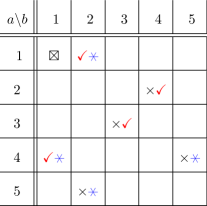
Figure 5: An illustration of Lemma 3: Suppose a round initialized with $\hat{a}=1$ and $\hat{b}=1$ such that $f^{xy}(\hat{a})=\hat{b}$ ($\square$). Such a permutation on the set $[d=5]$ is indicated with crosses ($\times$). The corresponding permutation $f^{(x,\hat{a})(y,\hat{b})}$ is shown with check-marks (✓). The relabelings $r_{\hat{a}=1}$ and $r_{\hat{b}=1}$ correlate $(5,2)$ by $(1,2)$ and $(4,5)$ by $(4,1)$ (indicated by $\hexstar$). Therefore, this round ends with only correct pairs that occur uniformly at random.

Thus, the round establishes local values $a_{t},b_{t}$ for which $f^{xy}(a_{t})=b_{t}$ holds. It is easy to see that each pair is equally probable, that is, happens with probability $1/d$. Therefore the round reproduces the joint distribution $D^{xy}_{AB}$ correctly.∎

See Figure 5 for an illustration of Lemma 3. We now prove that the presented protocol achieves an arbitrarily good simulation of any $D\in\mathcal{D}$ using a finite supply of approximations to $D^{\prime}(D)$, which are not too faulty.

Lemma 4.

It holds that $\mathcal{R}\leadsto^{\varepsilon}\mathcal{D}$.

Proof.

According to the simulation game setup two players are given the description of any target system in $\mathcal{D}$ with output alphabet $[d]$, where $d>2$. We denote this target system with $D_{d}$. The two players have a supply of $n$ approximations to the system $D^{\prime}(D_{d})$ at their disposal. By executing the presented protocol for $D_{d}$ they simulate the system $S$ as shown in Figure 3. We measure the quality of their approximation by the distance $\delta(S,D_{d})$, as introduced in Definition 1.

If the players use $n$ error-free resource systems of the kind $D^{\prime}$, then, in each round, Lemmas 2 and 3 imply a probability of $(d-2)/d$ to reach a zero-error simulation of $D_{d}$. Therefore, the probability that a wrong correlation remains after $n$ subsequent rounds is at most $(2/d)^{n}$. So, we have

$$\delta(S,D_{d})<\left(\frac{2}{d}\right)^{n},$$ (15)

where we obtain a strict upper bound because we omitted the non-zero probability to guess a correct pair in the first round. However, if the players feed the simulation protocol with $n$ approximations (denoted $S_{d-1}$) to the resource $D_{d-1}=D^{\prime}$, the simulation error $\delta_{d-1}=\delta(S_{d-1},D_{d-1})$ needs to be taken into consideration.

In each round the current simulated resource system $S_{d-1}$ returns a pair of outcomes not according to its definition with a chance of at most $\delta_{d-1}$. In this case the round can terminate with a wrong pair. If the resource system returns a pair to the players as its specification $D_{d-1}$ dictates, then a wrong pair remains with probability $2/d$. Thus, on inputs $x,y$, an incorrectly initialized round does not succeed in simulating the distribution $D_{AB}^{xy}$ with probability at most $\delta_{d-1}+(1-\delta_{d-1})2/d$ (see Figure 6, left-hand side). A round starting with a correct pair can still be influenced by the faulty simulation of $D_{d-1}$. With a maximal probability of $\delta_{d-1}$ the initially correct pair gets corrupted (see Figure 6, right-hand side).

Figure 6: In the left tree are the transition probabilities if the round starts with a faulty pair (☹) and in the tree on the right side we illustrate the transitions in the case of a correct starting pair.

Let $\delta^{(n)}_{d}$ denote the final simulation error if we run the simulation protocol for $D_{d}$ on exactly $n>0$ resource systems, that is, for $n$ subsequent rounds. Then, for any $d>2$, one can derive the recursive formula

$$\delta^{(n)}_{d} <\delta_{d}^{(n-1)}\left(\delta_{d-1}+(1-\delta_{d-1})\frac{2}{d}\right)+(1-\delta^{(n-1)}_{d})\delta_{d-1}$$

$$=\delta^{(n-1)}_{d}(1-\delta_{d-1})\frac{2}{d}+\delta_{d-1}$$ (16)

with the trivial base cases $\delta_{2}=0$ and $\delta^{(0)}_{d}=1$. For the simplicity of the formula we assumed that the initial pair is wrong – ignoring the fact that with some non-zero probability the initial guess is correct – which results in a strict upper bound. The explicit form of the right hand side of (16) can be found easily and turns out to be

$$\delta^{(n)}_{d}<\left(\frac{2}{d}(1-\delta_{d-1})\right)^{n}+\delta_{d-1}\left(\frac{\left(\frac{2}{d}(1-\delta_{d-1})\right)^{n}-1}{\frac{2}{d}(1-\delta_{d-1})-1}\right)$$ (17)

with the straightforward limiting expression

$$\lim_{n\rightarrow\infty}\delta^{(n)}_{d}<\frac{d\delta_{d-1}}{d-2+2\delta_{d-1}},$$ (18)

for large $n$. This expresses the intuitive fact that the distance of the actual simulated resource systems from their specification restricts the success of the shown simulation protocol.

We will now show that there always exists a finite number of resources, departing from their specifications with a certain non-zero distance $\delta_{d-1}$, that suffice for simulating $D_{d}$ to any desired quality $\delta_{d}>\lim_{n\rightarrow\infty}\delta^{(n)}_{d}$.

First, it follows from (17) that the simulation of any given system $D_{3}\in\mathcal{D}$ within the maximal distance $\delta_{3}=(2/3)^{n_{3}}$ can be achieved with $n_{3}$ copies of the resource system $D^{\prime}(D_{3})\in\mathcal{R}$. Generally, it is convenient for the following analysis and in accordance with the limit (18), to choose, for any $d>3$, the number of rounds as

$$n_{d}=\lceil\log_{\frac{2}{d}(1-\delta_{d-1})}\delta_{3}\rceil,$$ (19)

where obviously $\delta_{2}=0$. With this choice of $n_{d}$ the upper bound on the distance $\delta_{d}=\delta_{d}^{(n_{d})}$ becomes

$$\delta_{d}<\delta_{3}+\frac{\delta_{d-1}d(1-\delta_{3})}{d-2+2\delta_{d-1}}.$$ (20)

This recursive distance bound yields, after some simplifications, the explicit bound

$$\delta_{d}<\delta_{3}d^{2},$$ (21)

which is greater or equal to $\lim_{n\rightarrow\infty}\delta^{(n)}_{d}$ if $\delta_{d-1}\leq 1$. So, an initial distance of

$$\delta_{3}=\frac{\delta_{d}}{d^{2}}$$ (22)

is sufficient to guarantee a final distance below $\delta_{d}$. Therefore, for an arbitrary $\delta_{d}>0$ and an alphabet size $d>2$, we calculate $\delta_{3}$ by (22). From (20) and (21), with fixed values $\delta_{d}$ and $\delta_{3}$, the existence of a sufficiently small, non-zero distance $\delta_{d-1}$ is implied.

We conclude that, for any desired $\delta_{d}$ with $d>2$, there is always a finite number $n_{d}$ – given by (19) – of approximations to the resource system $D^{\prime}(D_{d})$ with a certain non-zero distance $\delta_{d-1}$, such that our protocol achieves the simulation of $D_{d}$ in the required quality. Since any finite amount of all $D_{2}\in\mathcal{R}$ is available in perfect quality to the players, the statement in the lemma follows by induction.∎

We finish with a performance estimate of the shown simulation in terms of the targeted distance $\delta_{d}$, for any $d>2$, and the number of needed resource systems from $\mathcal{R}$. To reach the system $D_{d}$ the simulation protocol is used $d-2$ times to increase the size of the output alphabet from 2 to $d$ in each step by 1. In this stepwise procedure the simulation error grows according to (20) and reaches a distance bounded as in (21) after $d-2$ steps. With

$$\prod_{i=3}^{d}n_{i}\leq\left\lceil\log_{\frac{2}{3}}\delta_{3}\right\rceil^{d}=\left\lceil\log_{\frac{3}{2}}\frac{d^{2}}{\delta_{d}}\right\rceil^{d}$$ (23)

resources from $\mathcal{R}$ our protocol thus simulates a system with a maximal distance of $\delta_{d}>0$ from the target $D_{d}$.

III.2 Interconverting $\mathcal{D}$ and $\mathcal{P}^{b}$

It is the purpose of the following part to close the gap between the set of permutation systems $\mathcal{D}$ and the set of all bipartite systems $\mathcal{P}^{b}$.

We show that two players, having the complete set $\mathcal{D}$ available as a resource, can simulate any bipartite system to an arbitrarily small distance. For any given $P\in\mathcal{P}^{b}$ we will construct a single resource $D(P)\in\mathcal{D}$ on which Alice and Bob can perform this task.

Lemma 5.

It holds that $\mathcal{D}\leadsto^{\varepsilon}\mathcal{P}^{b}$.

Proof.

Suppose we are given a target system $P\in\mathcal{P}^{b}$ with input alphabets $\mathcal{X}$, $\mathcal{Y}$ and output alphabets $\mathcal{A}$, $\mathcal{B}$. The task is to find an integer $d$ and a system $D(P)\in\mathcal{D}$ with the output set $[d]$, or equivalently, a set of permutations $\{f_{xy}:x\in X,y\in Y\}$ on $[d]$, such that, for all inputs $x,y$, the distribution $P^{xy}_{AB}$ can be reproduced by local operations on $D(P)$.

If $P$ contains any irrational probabilities, then we proceed with an arbitrarily close approximation to $P$ that is defined by rational probabilities only. In this special case the simulation will necessarily deviate from the specification and therefore the general result $\mathcal{R}\leadsto^{\varepsilon}P$ holds. Otherwise, we can construct exact simulations, that is, we can prove the reduction $\mathcal{R}\leadsto P$ for entirely rational target systems.

We construct $D(P)\in\mathcal{D}$ as follows. First, we choose $d$ to be the least common denominator (lcd) of all probabilities described by the system $P$. It is calculated as the smallest positive integer that is a multiple of all denominators. Therefore, we define

$$d:=\text{lcd}\{P_{AB}^{xy}(a,b):x\in\mathcal{X},y\in\mathcal{Y},a\in\mathcal{A},b\in\mathcal{B}\}.$$

Second, we fix local relabelings for given inputs $x,y$, that map all pairs $(a,b)$, identified through $f^{xy}(a)=b$, to a certain correlation according to $P^{xy}_{AB}$. For any given $x$ let Alice’s local relabeling function be denoted by

$$r^{x}_{A}:[d]\rightarrow\mathcal{A}.$$

On input $x$, $r^{x}_{A}$ maps, for each $a\in\mathcal{A}$, exactly $dP_{A}^{x}(a)$ unique elements of the set $[d]$ (the output set of $D(P)$) to the value $a$. And similarly for Bob. For any given input $y$ let the function

$$r^{y}_{B}:[d]\rightarrow\mathcal{B},$$

denote Bob’s local relabeling of outputs from $D(P)$. On input $y$, $r^{y}_{B}$ maps, for each $b\in\mathcal{B}$, exactly $dP_{B}^{y}(b)$ unique elements of the set $[d]$ to the value $b$. Once the relabelings $r_{A}^{x},r_{B}^{y}$ are fixed for all $x,y$, we can directly derive matching permutations $f^{xy}$, for any $x,y$, such that the corresponding system $D(P)$ is transformed into $P$ by the protocol consisting of the predefined local relabelings of outputs (this idea is illustrated in Figure 7).

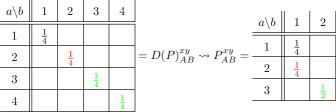
Figure 7: Here, we illustrate the simulation of an example distribution $P_{AB}^{xy}$ by local relabelings on the outputs of the distribution $D(P)^{xy}_{AB}$ when given fixed inputs $x,y$. Alice relabels local outputs from $D(P)^{xy}_{AB}$ as $r_{A}^{x}(1)=1,r_{A}^{x}(2)=2,r_{A}^{x}(3)=3$ and $r_{A}^{x}(4)=3$. Similarly, Bob relabels according to $r_{B}^{y}(1)=1,r_{B}^{y}(2)=1,r_{B}^{y}(3)=2$ and $r_{B}^{y}(4)=2$. Doing so, the players reproduce $P_{AB}^{xy}$ exactly.

Suppose fixed inputs $x,y$. For each pair $(a,b)\in\mathcal{A}\times\mathcal{B}$ in the support of $P^{xy}_{AB}$, let $f^{xy}$ correlate a number of $dP^{xy}_{AB}(a,b)$ unique outcomes $a^{\prime},b^{\prime}\in[d]$, that is, $f^{xy}(a^{\prime})=b^{\prime}$, such that $r_{A}^{x}(a^{\prime})=a$ and $r_{B}^{y}(b^{\prime})=b$. Since each output is correlated only once, it follows directly that $f^{xy}$ is a permutation and that, after the relabeling, all probabilities $P^{xy}_{AB}(a,b)$ are recovered. Therefore, we can simulate any wanted $P$ to an arbitrary precision by a simulation protocol on the system $D(P)\in\mathcal{D}$.∎

III.3 Interconverting $P_{PR}$ and $\mathcal{P}^{b}$

Putting the three pieces together we are now ready to state the main theorem of this section.

Theorem 1.

It holds that $P_{PR}\leadsto^{\varepsilon}\mathcal{P}^{b}$.

Proof.

From a finite supply of PR boxes any system in $\mathcal{R}$ can be simulated perfectly van Dam (2005). We described protocols on transforming a finite quantity of copies of a corresponding resource system in $\mathcal{R}$ into any system in $\mathcal{D}$ up to any desired maximal simulation distance (Lemma 4). Finally, any bipartite system can be simulated by Alice and Bob using a certain system from $\mathcal{D}$ and local operations (Lemma 5). The final simulation is not error-free if the target system contains irrational probabilities. Concluding, given enough PR boxes to the disposal of Alice and Bob, the two can agree on a classical strategy such that any wanted bipartite system is approximated within an arbitrarily small distance from its specification. ∎

We finish the section with some remarks concerning the efficiency of the shown procedure. Van Dam’s construction implies that for a target system in $\mathcal{R}$ with input alphabets $\mathcal{X}$ and $\mathcal{Y}$, where w.l.o.g. $|\mathcal{X}|\geq|\mathcal{Y}|$, one requires a supply of at most $|\mathcal{X}|$ PR boxes. It follows from our reduction $\mathcal{R}\leadsto^{\varepsilon}\mathcal{D}$ that for simulating a target system $D_{d}\in\mathcal{D}$, with output alphabet size $d$ and input sets $\mathcal{X}$ and $\mathcal{Y}$, we require a number of systems from $\mathcal{R}$ with input set cardinalities $d!|\mathcal{X}|/2$ and $d!|\mathcal{Y}|/2$. Therefore, using (23), the simulation of $D_{d}$, with a maximal input cardinality of $|\mathcal{X}|$, to the maximal distance $\delta_{d}$, costs at most

$$\left\lceil\log_{\frac{3}{2}}\frac{d^{2}}{\delta_{d}}\right\rceil^{d}\cdot\frac{d!}{2}|\mathcal{X}|$$

PR boxes. The final reduction $\mathcal{D}\leadsto^{\varepsilon}\mathcal{P}^{b}$ is a one to one relation. We simulate any $P\in\mathcal{P}^{b}$ with a related system $D_{d}(P)\in\mathcal{D}$ to a distance $\delta\leq\delta_{d}+(1-\delta_{d})\delta_{I}$. Here, $\delta_{I}$ stands for the error probability implied by the replacement of irrational probabilities in $P$ with rational approximations. Therefore, with the input cardinality $|\mathcal{X}|$ untouched by this reduction, we get that:

Theorem 2.

Any system $P\in\mathcal{N}_{2}$, with a maximal input set $\mathcal{X}$, can be simulated by two separated players to any distance $\delta>0$ with

$$\left\lceil\log_{\frac{3}{2}}\frac{d^{2}(1-\delta_{I})}{(\delta-\delta_{I})}\right\rceil^{d}\cdot\frac{d!}{2}|\mathcal{X}|$$

copies of a PR box as shared resources.

The choice for $\delta_{I}<\delta$ is arbitrary but implies a minimal size for the parameter $d$ depending on the actual irrational probabilities that need to be approximated. Roth’s inequality Roth (1955), an important result in the field of Diophantine approximations, provides such a lower bound .

None of the shown simulations claims to be optimal in the consumption of resources, neither does Van Dam’s construction. To our present knowledge it is an open question if the simulation can be improved to run on a number of PR boxes which is at most exponential in $d$.

IV A bipartite unit of nonlocality

As a natural follow-up we now extend the search for a unit to the space of target systems with more than two ends. Here, we investigate if, as it is the case in the bipartite simulation setting, there exists a set of bipartite resource systems such that a number of separated players can simulate any desired multipartite nonsignaling correlation arbitrarily well.

First, we introduce some additional definitions that will be used throughout this section.

Definition 6.

Let a (partial) assignment of values to a set of $n$ variables be denoted by $\rho\in(\mathbb{R}\cup\{*\})^{n}$, where $\rho[v]=*$ means that the variable $v$ remains unassigned by the partial assignment $\rho$.

If convenient we will sometimes write $\rho(V)$ for any assignment of values to the specified set $V$ of variables, while leaving the rest unassigned ($*$). An example: For $n=3$ we understand the assignment $\rho=(0,1,*)$ as the mapping from the variables $(v_{1},v_{2},v_{3})$ to $(0,1,*)$, that is, $v_{1}=0,v_{2}=1$ and $v_{3}$ unassigned. Equivalently, one may write $\rho(v_{1},v_{2})=(0,1)$.

Definition 7.

For any (partial) assignment $\rho$ let $l(\rho)$ denote the number of variables that are fixed by $\rho$. Formally,

$$l(\rho):=|\{v:\rho[v]\neq*\}|.$$

Suppose the inputs to some function $f:X\rightarrow Y$ are drawn from a probability distribution.

Definition 8.

For any (partial) assignment $\rho$ of values to the inputs of $f$ let $f|_{\rho}$ denote the random variable for the result of $f$ under the condition $\rho$. The probability distribution for all $y\in Y$ is straightforwardly given by

$$P(f|_{\rho}=y)=P(f=y|\rho).$$

Definition 9.

For any Boolean function $f$ and any (partial) input assignment $\rho$, let $\mu(f|_{\rho})$ denote the probability that $f$ evaluates to the minority decision conditioned on the assignment $\rho$. Formally, we define

$$\mu(f|_{\rho}):=\min(P(f|_{\rho}=0),P(f|_{\rho}=1)).$$

For the next definition we suppose a fixed adaptive simulation protocol in which an arbitrary player $j\in[m]$ shares $n$ resource systems $R_{1},...,R_{n}$ with the rest of the players.

Definition 10.

For any input $x_{j}$ and any index $i\in[n]$, let the set $S_{i}(x_{j})$ include all those partial assignments $\rho$ to the shared variable $\lambda$ and the binary variables $b_{1},\ldots,b_{n}$, that, according to player $j$’s wiring, imply $i$ as the index of the next system to use. Formally, for any $i$, we define

$$S_{i}(x_{j}):=\{\rho\in\mathbb{R}\times\{0,1,*\}^{n}:i_{l(\rho)}(x_{j},\rho)=i\}.$$

We can now start with the statements and proofs of the present section.

IV.1 Non-adaptive protocols

In what follows, a counter example is derived, that is, a simulation game that cannot be played arbitrarily well under certain constraints. We consider the simulation of the target system $T$ (Example 1). The five involved players are restricted to agree on non-adaptive simulation protocols only and have the resource set $\mathcal{P}^{b}$ available. As the main result of this subsection, it is shown in Corollary 1 that the minimal departure $\delta(S,T)$ of any system $S$, simulated under these conditions, from the target $T$, is bounded away from 0.

We use the following notation: Player $i$ shares $n$ resource systems in total and of these $n_{j}\leq n$ resource systems $R_{1},\ldots,R_{n_{j}}$ with player $j$ in particular. During the simulation game, player $i$ is given input $x_{i}$ and the shared random value $\lambda$, drawn from some distribution $P_{\Lambda}$. The outputs of the resource systems shared with player $j$ are assigned to the local variables $b_{1},\ldots,b_{n_{j}}$, which are part of the overall local sequence $b_{1},\ldots,b_{n}$. The output of player $i$ is determined by $f^{x_{i}}(\lambda,b_{1},\ldots,b_{n})$.

For Lemma 6 we allow only simulation protocols of a special kind and generalize the results later in Corollary 1. We suppose any simulation protocol for $T$ executed by five players on resources from $\mathcal{R}$ with the following input-dependence constraint: Each player determines the inputs into systems shared with player $j$ independently of the outputs obtained from systems shared with player $j^{\prime}$, for all distinct $j,j^{\prime}\in[5]$.

Lemma 6 expresses the fact that the dependence of a player’s output on the local outputs of the resource systems shared with another player implies a violation of $T$’s correlation conditions (stated in Example 1) and, therefore, a certain related simulation distance. It is an adaptation of Theorem 2 by Barrett and Pironio Barrett and Pironio (2005) to approximate reductions.

Lemma 6.

Take any pair of distinct players $i,j\in[5]$. Any simulated system $S$ departs from the target $T$ with distance

$$\delta(S,T)\geq\sum_{\rho}P(\rho)\mu(f^{0}|_{\rho}),$$

where $f^{0}$ is player $i$’s output function on input $0$ and we sum over all partial assignments $\rho=\rho(\lambda,b_{n_{j}+1},\ldots,b_{n})$ to player $i$’s local variables.

Proof.

We prove the statement for an exemplary pair of players. The reasoning extends to any other pair by a simple argument, as explained later.

Let us choose the pair $i=1,j=2$ and analyze the situation from player 1’s perspective on input $x_{1}=0$. Note that from the definition of the target system and the resources it follows that the sequence $b_{1},\ldots,b_{n}$ is a uniformly distributed random binary string of length $n$ and $f^{0}$ – player 1’s local output function on input 0 – is a Boolean function.

Since $x_{1}=0$, we have that if $x_{4}=0$ and $x_{5}=1$, then correlation (4) of Example 1, that is,

$$a_{4}+a_{5}+a_{1}\equiv 0~{}(\text{mod }2)$$ (24)

needs to be fulfilled by the final outputs of the players. Conditioned on any assignment $\rho=\rho(\lambda,b_{n_{2}+1},\ldots,b_{n})$, the result of $f^{0}$ depends solely on the remaining variables $b_{1},\ldots,b_{n_{2}}$. In other words, it depends on the outcomes of systems shared with player 2, who is not involved in the above correlation. If player 2’s actions on these systems would influence the simulation of (24), then players 1,4, and 5 could team up and receive signals from player 2. Since $\mathcal{R}\subset\mathcal{P}$ holds, this is impossible. We can thus assume that player 2 does not provide inputs to the systems shared with player 1 while sustaining the simulation of (24). Therefore, conditioned on $x_{1}=0$ and any $\rho$, player 1’s output is basically a local random bit that is 1 with probability $P(f^{0}|_{\rho}=1)$.

Let $\rho_{i}$ denote an assignment of values to all outputs of resource systems that are received by players $[5]\backslash\{i\}$. If we fix their inputs, the shared random value $\lambda$ and $\rho_{i}$, then the outputs of these players are determined.

Suppose now fixed inputs $x_{1}=0,x_{2},x_{3},x_{4}=0,x_{5}=1$ and a fixed shared value $\lambda$. Conditioned on any $\rho_{1}$, player 1’s correct output is uniquely given by (24), the other output implies a violation of this correlation. For any $\rho$ and $\rho_{1}$, (24) is thus violated with a probability of at least $\mu(f^{0}|_{\rho})$. In all protocols considered here player 1’s inputs into systems $R_{n_{2}+1},\ldots,R_{n}$ are independent of $b_{1},\ldots,b_{n_{2}}$. Therefore, the distribution of the random variable $f^{0}|_{\rho}$ is independent of $\rho_{1}$. The convex combination of all possible events $\rho$ and $\rho_{1}$ yields

$$\delta(S,T) \geq\sum_{\rho,\rho_{1}}P(\rho,\rho_{1})\mu(f^{0}|_{\rho})$$

$$=\sum_{\rho}P(\rho)\mu(f^{0}|_{\rho}).$$

This argument extends to any pair of players because one can always find a correlation among (1)-(6) in which only one of the players is involved on input 0. ∎

It is now clear that using resource systems from $\mathcal{R}$ in a simulation of $T$ guarantees a distance related to the players’ output functions. When a player only considers its initial input and the shared random value for a final output decision, we expect the simulation distance to be higher. However, this increase might still be within a constant factor of the lower bound derived above. This is the idea leading to the following theorem. Again, we consider any simulation protocol for the target correlation $T$ executed by 5 separated players on a finite amount of copies of a resource system from $\mathcal{R}$ that fulfills the input dependence constraint mentioned before.

Theorem 3.

There exists a constant $c$ such that from any simulation protocol with distance $\delta$ the existence of a local system with distance at most $c\delta$ follows.

Proof.

The initial protocol simulates a system $S$ which approximates $T$ with distance $\delta(S,T)$.

Consider player 1 first. We build a new protocol by changing player 1’s local output function as follows: Conditioned on input $x_{1}=0$ and any assignment $\rho=\rho(\lambda,b_{n_{2}+1},\ldots,b_{n})$, the new function shall constantly output the majority of the outputs of the original function under the same condition, that is,

$$\hat{f}^{1}|_{\rho} =f^{1}|_{\rho},$$

$$\hat{f}^{0}|_{\rho} =\begin{cases}1,\text{ if }P(f^{0}|_{\rho}=1)\geq\frac{1}{2},\\ 0,\text{ otherwise}.\end{cases}$$

Obviously, $\hat{f}^{0}$ is independent of the values $b_{1},\ldots,b_{n_{2}}$ – the actual system outputs correlated with player 2 – for it depends only on the related output distribution. One can calculate the increase in the simulation distance that is implied by this change. Assume a choice of inputs with $x_{1}=0$ that demands a certain correlation with player 1 involved. Conditioned on any $\rho$, replacing $f^{0}$ by $\hat{f}^{0}$ can increase the chance of violating this correlation by at most the probability that the minority output is generated by the original function, hence $\mu(f^{0}|_{\rho})$. Otherwise, player 1’s output behavior has not changed at all. So, summing over all possible $\rho$, the change increases the simulation distance by at most

$$\sum_{\rho}P(\rho)\mu(f^{0}|_{\rho}).$$

Lemma 6, with parameters $i=1,j=2$, implies that the distance $\delta(S,T)$ of the original simulation protocol is already at least as high. Therefore, our change doubles the simulation distance in the worst case. Thus, the new simulation protocol approximates $T$ with a distance within $2\delta(S,T)$.

With the same argument on different pairs involving player 1 we change the protocol another three times. We sequentially free player 1’s output function on input $x_{1}=0$ from the dependence on outputs of shared resource systems. Doing so, we obtain a new simulation protocol for $T$ with a simulation distance bounded by $2^{4}\delta(S,T)$. Then, we extend this procedure to all players. Finally, we reach a protocol where each players’ output is independent of the outputs of its shared resource systems if getting input 0. The new simulation distance is limited by $2^{20}\delta(S,T)$.

We continue the reasoning with the new simulation protocol. Now assume player 1 gets input $x_{1}=1$. If $x_{2}=x_{5}=0$, then correlation (5) of Example 1, that is,

$$a_{5}+a_{1}+a_{2}=0~{}(\text{mod }2),$$ (25)

needs to be fulfilled by the outputs of the players. In the current version of the protocol, all players base their outcome solely on the shared value $\lambda$ when getting the input $0$, as do players $2$ and $5$. Conditioned on a $\lambda$, player 1’s output function $f^{1}$ will, therefore, determine an output not satisfying (25) with a probability of at least $\mu(f^{1}|_{\lambda})$. Therefore, the simulation distance of the new protocol is bounded from below by the convex combination of these values, that is, by

$$\sum_{\lambda}P_{\Lambda}(\lambda)\mu(f^{1}|_{\lambda}).$$ (26)

For each $\lambda$, $f^{1}$ is now replaced by a function evaluating to the majority decision of $f^{1}|_{\lambda}$, similarly to the modifications made earlier. This change establishes that player 1’s output function is independent of the outputs of all shared resource systems $R_{1},\ldots,R_{n}$. For each $\lambda$, which is the shared value with chance $P_{\Lambda}(\lambda)$, this causes a simulation distance increase which is maximally as large as the probability of player 1’s minority decision given $x_{1}=1$ and $\lambda$, that is, $\mu(f^{1}|_{\lambda})$. The total increase is then maximally as large as (26). Therefore, the new protocol, in which player 1’s strategy relies only on shared randomness, is at most twice as faulty as the old one.

With the same argument we handle players’ $2,3,4$ and $5$’s dependence on resource system outputs. As seen above we pay these changes with a factor of at most $2^{4}$ in the simulation distance. Therefore, the final protocol for $T$ relies only on shared randomness and simulates a certain local system $S^{\prime}$ with $\delta(S^{\prime},T)\leq 2^{25}\delta(S,T)$.∎

Corollary 1.

There is at least one multipartite system that cannot be approximated arbitrarily well with a non-adaptive protocol on bipartite systems.

Proof.

An example is $T$. Assume that there is a non-adaptive protocol on resources from $\mathcal{P}^{b}$ simulating a system $S$ that approximates $T$ arbitrarily well, that is, with any $\delta(S,T)>0$. We replace all bipartite systems used in this protocol by simulations on the resource set $\mathcal{R}$. This can be achieved asymptotically perfect by a combination of simulation protocols demonstrated in Section III. It is a fact that one of the needed reductions ($\mathcal{R}\leadsto^{\varepsilon}\mathcal{D}$) uses adaptive protocols. However, since these simulations are bipartite, the non-adaptive nature of the assumed protocol on $\mathcal{P}^{b}$ translates into the constrained input dependence as required in Lemma 6 and Theorem 3.

It then follows directly from Theorem 3 that there is a local system that approximates $T$ to an arbitrary precision. This contradicts the established fact that $T$ violates a Bell inequality DiVincenzo and Peres (1997). ∎

IV.2 Adaptive protocols

Next, we consider the general case where the players of the simulation game are allowed to agree on any kind of protocol. We will show that the same example, which was impossible to approximate in the restricted setting, is a hard instance in the general case as well. This will be demonstrated by deriving a lower bound on the distance that occurs when five players simulate the target $T$ on shared randomness and a finite amount of copies of systems from $\mathcal{R}$. We find a distance bound that can theoretically reach any small value but decreases rather slowly, that is, reciprocally in the number of shared resources.

As a first step into this direction, we show a weaker lower bound that has not yet the required property but will be useful later. For $i\in[n]$, let $\delta(S,T|i)$ denote the simulation distance of a protocol conditioned on the assumption that any player’s variable $b_{i}$ is determined locally and uniformly at random.

Lemma 7.

Suppose any choices $j\in[5]$, $x_{j}\in\{0,1\}$ and $i\in[n]$. In a simulation protocol for $(T,\mathcal{R})$ in which player $j$’s binary variable $b_{i}$ is assigned the result of a local, fair coin toss, we have that

$$\delta(S,T|i)\geq\sum_{\rho\in S_{i}(x_{j})}P(\rho)[\mu(f^{x_{j}}|_{\rho}) -\tfrac{1}{2}\mu(f^{x_{j}}|_{\rho,b_{i}=0})$$

$$-\tfrac{1}{2}\mu(f^{x_{j}}|_{\rho,b_{i}=1})].$$

Proof.

Informally spoken, the conditional distance $\delta(S,T|i)$ is at least half as high as the minimal probability, for any fixed inputs, that player $j$’s output changes depending on his local bit $b_{i}$, while the outputs of the other players remain constant.

For the rest of the proof we fix the players’ inputs such that their outputs have to satisfy a correlation from (1) – (6) with player $j$ involved. Let $\rho_{j}$ denote an assignment of values to all outputs of resource systems that are received by players $[5]\backslash\{j\}$. Fixing $\rho_{j}$ and the shared random value $\lambda$ determines the output of these players. If player $j$’s output remains variable, then a violation of the required correlation occurs. Given $x_{j}$ and an assignment $\rho\in S_{i}(x_{j})$ (see Definition 10), it is convenient to introduce the random variables $\xi=f^{x_{j}}|_{\rho,b_{i}=0}$ and $\zeta=f^{x_{j}}|_{\rho,b_{i}=1}$. We have $P(\xi=a)=P(f^{x_{j}}=a|b_{i}=0,\rho)$ and $P(\zeta=a)=P(f^{x_{j}}=a|b_{i}=1,\rho)$ forn all outputs $a\in\{0,1\}$. The probability of the described violation can then be stated as

$$\delta(S,T|i)\geq\frac{1}{2}\sum_{\rho\in S_{i}(x_{j})}\sum_{\rho_{j}}P(\rho,\rho_{j})P(\xi\neq\zeta|\rho_{j}).$$ (27)

Here, $P(\xi\neq\zeta|\rho_{j})$ denotes the probability that player $j$’s output when obtaining $\rho$ and then $b_{i}=0$ differs from the output in the case $\rho$ and $b_{i}=1$, conditioned on $\rho_{j}$. Assume $\rho$ to be fixed for the moment. Since $f^{x_{j}}$ is a Boolean function, $P(\xi\neq\zeta|\rho_{j})$ can be decomposed into two basic cases.

$$P(\xi\neq\zeta|\rho_{j})=P(\xi=0,\zeta=1|\rho_{j})+P(\xi=1,\zeta=0|\rho_{j}).$$ (28)

Next, we observe that for all $a$ the events $\xi=a$ and $\zeta=\bar{a}$ conditioned on $\rho_{j}$ are independent because $b_{i}=0$ and $b_{i}=1$ are mutually exclusive conditions. Therefore,

$$P(\xi=a,\zeta=\bar{a}|\rho_{j})=P(\xi=a|\rho_{j})P(\zeta=\bar{a}|\rho_{j})$$ (29)

holds for any $\rho_{j}$. From now on let $a$ be such that $\mu(f^{x_{j}}|_{\rho})=P(f^{x_{j}}=a|\rho)$, that is, $a$ is the least probable output under the condition $\rho$. It is easy to see that (29) can be rewritten to

$$P(\xi=a,\zeta=\bar{a}|\rho_{j})= P(\xi=a|\rho_{j})$$

$$-P(\xi=a|\rho_{j})P(\zeta=a|\rho_{j})$$

and therefore, applied to (28), we get the equality

$$P(\xi\neq\zeta|\rho_{j}) =P(\xi=a|\rho_{j})+P(\zeta=a|\rho_{j})$$

$$-2P(\xi=a|\rho_{j})P(\zeta=a|\rho_{j})$$

$$=2P(f^{x_{j}}=a|\rho,\rho_{j})$$

$$-2P(\xi=a|\rho_{j})P(\zeta=a|\rho_{j}).$$

Now we choose the bit $b_{i}$ such that the term $\sum_{\rho_{j}}P(\rho_{j}|\rho)P(f^{x_{j}}=a|\rho,b_{i},\rho_{j})$ is minimal, one easily obtains the lower bound

$$P(\xi\neq\zeta|\rho_{j})\geq 2P(f^{x_{j}}=a|\rho,\rho_{j})-2P(f^{x_{j}}=a|\rho,b_{i},\rho_{j})$$

for any $\rho_{j}$. Let $\bar{\rho}$ denote any assignment of the remaining variables in $b_{1},\ldots,b_{n}$ not fixed by $\rho$. Observe that for any assignments $\rho,\rho_{j}$ we have

$$P(f^{x_{j}}=a|\rho,\rho_{j}) =\sum_{\bar{\rho}}P(\bar{\rho},f^{x_{j}}=a|\rho,\rho_{j})$$

$$=\sum_{\bar{\rho}}P(\bar{\rho}|\rho,\rho_{j})\mathbf{1}_{f^{x_{j}}=a}(\rho,\bar{\rho}),$$

where $\mathbf{1}_{f^{x_{j}}=a}(\rho,\bar{\rho})\in\{0,1\}$ indicates whether $f^{x_{j}}(\rho,\bar{\rho})$ evaluates to $a$. For any fixed $\rho$ this implies

$$\sum_{\rho_{j}} P(\rho_{j}|\rho)P(f^{x_{j}}=a|\rho,\rho_{j})$$

$$=\sum_{\rho_{j}}P(\rho_{j}|\rho)\sum_{\bar{\rho}}P(\bar{\rho}|\rho,\rho_{j})\mathbf{1}_{f^{x_{j}}=a}(\rho,\bar{\rho})$$

$$=\sum_{\rho_{j},\bar{\rho}}P(\rho_{j},\bar{\rho}|\rho)\mathbf{1}_{f^{x_{j}}=a}(\rho,\bar{\rho})$$

$$=\sum_{\bar{\rho}}P(\bar{\rho}|\rho)\mathbf{1}_{f^{x_{j}}=a}(\rho,\bar{\rho})=P(f^{x_{j}}=a|\rho).$$

Thus, (27) becomes

$$\delta(S,T|i)\geq ~{}\sum_{\rho}P(\rho)P(f^{x_{j}}=a|\rho)$$

$$-\sum_{\rho,\rho_{j}}P(\rho,\rho_{j})P(f^{x_{j}}=a|\rho,b_{i},\rho_{j}).$$

This is almost the representation we seek. Now, as a last step, we will get rid of the second dependence on $\rho_{j}$ by using the initial assumption on $b_{i}$. Let now $\bar{\rho}$ stand for any assignment of the remaining variables in $b_{1},\ldots,b_{n}$ not fixed by $\rho$ and not equal to $b_{i}$. Observe that for any assignments $\rho,\rho_{j}$ and any $b_{i}$ it holds that

$$P(f^{x_{j}}=a|\rho,b_{i},\rho_{j}) =\sum_{\bar{\rho}}P(\bar{\rho},f^{x_{j}}=a|\rho,b_{i},\rho_{j})$$

$$=\sum_{\bar{\rho}}P(\bar{\rho}|\rho,b_{i},\rho_{j})\mathbf{1}_{f^{x_{j}}=a}(\rho,b_{i},\bar{\rho}).$$

Using the equality $P(\rho_{j}|\rho)=P(\rho_{j}|\rho,b_{i})$ – which holds only because $b_{i}$ is assumed to be determined locally at random, meaning that $P(b_{i})=P(b_{i}|\rho)=P(b_{i}|\rho,\rho_{j})$ – yields

$$\sum_{\rho_{j}} P(\rho_{j}|\rho)P(f^{x_{j}}=a|\rho,b_{i},\rho_{j})$$

$$=\sum_{\rho_{j},\bar{\rho}}P(\rho_{j},\bar{\rho}|\rho,b_{i})\mathbf{1}_{f^{x_{j}}=a}(\rho,b_{i},\bar{\rho})$$

$$=\sum_{\bar{\rho}}P(\bar{\rho}|\rho,b_{i})\mathbf{1}_{f^{x_{j}}=a}(\rho,b_{i},\bar{\rho})=P(f^{x_{j}}=a|b_{i},\rho).$$

Therefore, we can reformulate (27) to

$$\delta(S,T|i)\geq\sum_{\rho}P(\rho)[P(f^{x_{j}}=a|\rho)-P(f^{x_{j}}=a|b_{i},\rho)].$$

Remember that the variable $b_{i}$ has been assigned such that for each $\rho$ the probability $P(f^{x_{j}}=a|b_{i},\rho)$ is smaller or equal to $P(f^{x_{j}}=a|\bar{b}_{i},\rho)$. Therefore, using $\mu(f^{x_{j}}|_{\rho})=P(f^{x_{j}}=a|\rho)$ it is easy to derive the equality $P(f^{x_{j}}=a|b_{i},\rho)=\mu(f^{x_{j}}|_{\rho,b_{i}})$. Also, $\mu(f^{x_{j}}|_{\rho,b_{i}})\leq\mu(f^{x_{j}}|_{\rho,\bar{b}_{i}})$ holds since otherwise $\mu(f^{x_{j}}|_{\rho})=P(f^{x_{j}}=a|\rho)$ would not be satisfied. From this one can conclude

$$\delta(S,T|i)\geq\sum_{\rho}P(\rho)[\mu(f^{x_{j}}|_{\rho}) -\tfrac{1}{2}\mu(f^{x_{j}}|_{\rho,b_{i}=0})$$

$$-\tfrac{1}{2}\mu(f^{x_{j}}|_{\rho,b_{i}=1})]$$

which finishes the proof.∎

For a fixed $i$, the lower bound on the simulation error as given in Lemma 7 is independent of the number of resource systems used in the simulation and can be trivial, that is, equal to zero. The argument may be boosted by calculating a lower bound to the sum of all conditional distances. As we will see now this approach finally yields the linear dependence on the number of used resource systems.

Suppose an adaptive simulation protocol for $T$ on resources from $\mathcal{R}$ in which each player shares at most $n$ resource systems.

Lemma 8.

For any choices of $j\in[5]$ and $x_{j}\in\{0,1\}$, there is at least one index $i\in[n]$ such that

$$\delta(S,T|i)\geq\frac{1}{n}\sum_{\lambda}P_{\Lambda}(\lambda)2\mu(f^{x_{j}}|_{\lambda}).$$

Proof.

For any player $j$, we will show a lower bound to the sum of conditional distances, assuming for each summand a protocol in which the variable $b_{i}$ is determined locally and uniformly at random.

We will use $f$ for $f^{x_{j}}$ to avoid unnecessary lengths in the formulas. After fixing the inputs for the rest of the players accordingly, Lemma 7 implies

$$\sum_{i=1}^{n}\delta(S,T|i)\geq\sum_{i=1}^{n}\sum_{\rho\in S_{i}(x_{j})}P(\rho)[\mu(f|_{\rho}) -\tfrac{1}{2}\mu(f|_{\rho,b_{i}=0})$$

$$-\tfrac{1}{2}\mu(f|_{\rho,b_{i}=1})].$$

Introducing player $j$’s local function $\hat{i}=i_{l(\rho)}$ that, based on current local assignments $x_{j},\rho$, decides the index of the next (the $l(\rho)$th) system to use, we replace the right-hand side by

$$\sum_{\rho\in S(x_{j})}P(\rho)[\mu(f|_{\rho})-\tfrac{1}{2}\mu(f|_{\rho,b_{\hat{i}}=0})-\tfrac{1}{2}\mu(f|_{\rho,b_{\hat{i}}=1})],$$

where the set of all assignments is denoted by $S(x_{j})=\bigcup_{i=1}^{n}S_{i}(x_{j})$. Observe now that for any $\rho\in S_{i}(x_{j})$ and any assignment to $b_{i}$, which means for all $(\rho,b_{i}=0),(\rho,b_{i}=1)\in S(x_{j})$, we have

$$P(\rho,b_{i})\mu(f|_{\rho,b_{i}})=\tfrac{1}{2}P(\rho)\mu(f|_{\rho,b_{i}})$$

since $P(\rho,b_{i})=P(\rho)/2$. Furthermore, we will make use of the fact that for all $\rho\in S(x_{j})$, which fix $n-1$ local variables from $b_{1},\ldots,b_{n}$ and the shared value $\lambda$, we have $\mu(f|_{\rho,b_{i}=0})=\mu(f|_{\rho,b_{i}=1}))=0$. Therefore, all summands cancel each other out except the ones corresponding to initial assignments that fix only $\lambda$. Thus,

$$\sum_{i=1}^{n}\delta(S,T|i) \geq\sum_{\lambda}P_{\Lambda}(\lambda)\mu(f|_{\lambda})$$

which completes the proof.∎

It seems natural that the sum $\sum_{\lambda}P_{\Lambda}(\lambda)2\mu(f^{x_{j}}|_{\lambda})$, for at least one player $j\in[5]$, cannot be smaller than some constant related to the distance between $T$ and the closest local system. Otherwise, this local system would conflict with the fact that $T$ violates a Bell inequality. This intuition is formulated and confirmed by the following theorem.

Theorem 4.

Any simulation protocol for $T$ in which each player shares maximally $n$ resources from $\mathcal{R}$ with the rest of the players simulates a system $S$ with

$$\delta(S,T)\in\Omega(n^{-1}).$$

Proof.

We take the perspective of player $j\in[5]$, such that the sum

$$\sum_{\lambda}P_{\Lambda}(\lambda)\mu(f^{x_{j}=0}|_{\lambda})$$

is maximal. Player $j$ shares $n_{j}\leq n$ systems with the rest of the players. According to Lemma 8, there exists an index $i\in[n_{j}]$ identifying one of player $j$’s local variables, such that

$$\delta(S,T|i)\geq\frac{1}{n}\sum_{\lambda}P_{\Lambda}(\lambda)2\mu(f^{0}|_{\lambda}).$$

The system $R_{i}$ is shared with another player. It follows directly from the $T$’s correlation conditions (Example 1), that for $x_{j}=0$ it is always possible to choose inputs to the rest of the players such that player $j$ is, and the player with which system $R_{i}$ is shared is not, involved in the required correlation. By the nonsignaling principle we can assume that the other player with access to $R_{i}$ completely ignores its end of the system while sustaining the original simulation of the required correlation. Therefore, player $j$’s variable $b_{i}$, the output of $R_{i}$, can be interpreted as a local bit distributed uniformly at random. Thus, we obtain a lower bound to the simulation distance:

$$\delta(S,T)\geq\delta(S,T|i).$$ (30)

As in the non-adaptive case we change the local output functions of all players to depend only on shared randomness $\lambda$, when given the input $0$. Now, each player decides on the outcome with the greater probability, when conditioning its corresponding output function on $\lambda$. Thus, for each value of $\lambda$, a departure from the original protocol is as probable as a change in a player’s outcome behavior – the probability of the minority decision under $\lambda$. It follows that they now simulate a system $S^{\prime}$ with

$$\delta(S^{\prime},T)\leq\delta(S,T)+5\sum_{\lambda}P_{\Lambda}(\lambda)\mu(f^{0}|_{\lambda}).$$

Suppose this change has been adapted and the new simulation protocol is now executed instead. In a situation where player $j^{\prime}$ is given $x_{j^{\prime}}=1$, and the two other players also involved in the required correlation receive the input 0 (there is such a correlation condition for each choice $j^{\prime}\in[5]$), the correct output of player $j^{\prime}$ is determined as soon as $\lambda$ is fixed. Therefore,

$$\delta(S^{\prime},T)\geq\max_{j^{\prime}\in[5]}\sum_{\lambda}P_{\Lambda}(\lambda)\mu(f^{x_{j^{\prime}}=1}|_{\lambda}).$$

If we change the players’ output functions again, in such a way that they depend only on shared randomness given input $1$ as well, then they simulate a purely classical (local) system $S_{c}$ with a simulation distance of

$$\delta(S_{c},T) \leq\delta(S,T)+5\sum_{\lambda}P_{\Lambda}(\lambda)\mu(f^{0}|_{\lambda})$$

$$\hskip 44.10185pt+5\max_{j^{\prime}\in[5]}\sum_{\lambda}P_{\Lambda}(\lambda)\mu(f^{x_{j^{\prime}}=1}|_{\lambda})$$

$$\leq\delta(S,T)+5\sum_{\lambda}P_{\Lambda}(\lambda)\mu(f^{0}|_{\lambda})+5\delta(S^{\prime},T)$$

$$\leq 6\delta(S,T)+30\sum_{\lambda}P_{\Lambda}(\lambda)\mu(f^{0}|_{\lambda}),$$

which is at least as high as the minimal distance $\delta_{c}$ that can be achieved with a classical protocol. We conclude that either the original simulation protocol is bounded away from 0, for example by $\delta(S,T)>\delta_{c}/12$, or otherwise, if $\delta(S,T)\leq\delta_{c}/12$, then we have

$$\frac{\delta_{c}}{2}\leq 30\sum_{\lambda}P_{\Lambda}(\lambda)\mu(f^{0}|_{\lambda}).$$

Using inequality (30), this yields that any simulation protocol for $T$ on resources from $\mathcal{R}$ has a distance from the specification of

$$\delta(S,T) \geq\frac{1}{n}\sum_{\lambda}P_{\Lambda}(\lambda)\mu(f^{0}|_{\lambda})\geq\frac{1}{n}\cdot\frac{\delta_{c}}{60}.$$

∎

Theorem 4 implies that the error in any simulation of $T$ maximally decreases at rate that is reciprocal to the number of shared resources between two players. Hence, no simulation with finitely many bipartite resource systems can be perfect – a known fact that has already been proved in Barrett and Pironio (2005). Furthermore, it gives evidence that some multipartite quantum correlations are at least quite costly to approximate.

V Conclusions

In this work we proved and analyzed a possible way for two separated parties to transform a supply of shared PR boxes into any desired bipartite system. The simulation can be made arbitrarily accurate by increasing the number of resources. This establishes the PR box as a unit of bipartite nonlocality. An analysis of our scheme’s efficiency reveals that reducing the output alphabet is particularly expensive in terms of required resource systems. Furthermore, we derive limitations that any bipartite unit will encounter in the multipartite setting. We find that the asymptotic simulation of certain quantum correlations is impossible for players restricted to non-adaptive strategies. In the general case, we derive a lower bound to the simulation distance that drops reciprocally in the number of deployed resources. Informally speaking, this does not prevent adaptive protocols from reaching any small simulation distance but restricts to trading doubled simulation quality off at least twice as many resources. Note that $P_{PR}\in\mathcal{R}$ and $\mathcal{R}\subset\mathcal{P}^{b}$. Therefore, the bound also holds for PR boxes as resources. A possible generalization to arbitrary bipartite resource systems is a task left for future work. It still remains to identify a nontrivial set of nonsignaling correlations that can serve as a unit of multipartite nonlocality in the sense adopted in this work. Our results suggest that such a system has more than two ends. A promising candidate that comes to mind is the multipartite version of systems characterized by permutations – a generalization of the set $\mathcal{D}$. However, the simulations derived in this article seem to be unfit for a direct application.

Simulation protocols that amplify the violation of a CHSH inequality of given resource systems, so-called nonlocality distillation protocols, have been introduced in Forster et al. (2009) and since improved in Brunner and Skrzypczyk (2009); Høyer and Rashid (2010); Allcock et al. (2009). Here, we want to point out an interesting implication of these interconversions. The distillation protocol in Brunner and Skrzypczyk (2009) achieves an asymptotic simulation of a PR box through processing a finite supply of correlated nonlocal boxes, which are convex combinations of a PR box and perfectly correlated random bits. We must, therefore, conclude from Theorem 1 that each correlated nonlocal box is a unit of bipartite nonlocality in the same sense as the PR box. One may ask if inner points of the polytope of binary nonsignaling correlations could also serve as units. We cannot give a final answer to this question. However, oppositional evidence exists. If it holds true that there is no nonlocality distillation protocol for isotropic systems, as already shown for infinitely many examples in the quantum region Dukaric and Wolf (2008), then a negative answer follows directly from the general upper bound on distillable nonlocality derived in Forster (2011).