The dust un-biased cosmic star formation history from the 20 cm VLA-COSMOS survey

Abstract

We derive the cosmic star formation history (CSFH) out to $z=1.3$ using a sample of $\sim 350$ radio-selected star-forming galaxies, a far larger sample than in previous, similar studies. We attempt to differentiate between radio emission from AGN and star-forming galaxies, and determine an evolving 1.4 GHz luminosity function based on these VLA-COSMOS star forming galaxies. We precisely measure the high-luminosity end of the star forming galaxy luminosity function (SFR $\gtrsim 100\,M_{\sun}\,{\rm yr}^{-1}$; equivalent to ULIRGs) out to $z=1.3$, finding a somewhat slower evolution than previously derived from mid-infrared data. We find that more stars are forming in luminous starbursts at high redshift. We use extrapolations based on the local radio galaxy luminosity function; assuming pure luminosity evolution, we derive $L_{*}\propto(1+z)^{2.1\pm 0.2}$ or $L_{*}\propto(1+z)^{2.5\pm 0.1}$, depending on the choice of the local radio galaxy luminosity function. Thus, our radio-derived results independently confirm the $\sim 1$ order of magnitude decline in the CSFH since $z\sim 1$.

1. Introduction

Studies based on different galaxy star formation indicators (UV, optical, FIR, radio) agree that the cosmic star formation history (i.e. the total star formation rate per unit co-moving volume; CSFH hereafter) has declined by about an order of magnitude since $z\sim 1$ (for a compilation see e.g. Hopkins 2004). One of the major difficulties of UV/optical based tracers is the significant model-dependent dust-obscuration correction that needs to be imposed on the data. This ‘dust-obscuration problem’ may be overcome using longer wavelengths, such as the IR and radio regimes. However, in these cases a multi-wavelength approach is essential as redshift information and a reliable identifier of star forming (SF) galaxies is required (e.g. Caputi et al. 2007; Smolčić et al. 2008; S08 hereafter). In this context the radio star formation tracer provides an important complementary view of the CSFH. First, radio emission is a dust-insensitive tracer of recent star formation (not affected by old stellar populations; see Condon 1992 for a review). Second, interferometric radio observations with $\sim 1^{\prime\prime}$ resolution allow more reliable identifications (compared to FIR and sub-mm data) with objects detected at other wavelengths.

The dust-unbiased total CSFH has been constrained recently using MIR (24/8$\mathrm{\mu m}$) selected samples obtained by deep small area surveys (CDFS, GEMS, GOODS; Le Floc’h et al. 2005; Zheng et al. 2006, 2007; Caputi et al. 2007; Bell et al. 2007). Small area surveys, however, are subject to cosmic variance. Moreover, they do not observe a large enough comoving volume in order to fairly sample rare high-luminosity galaxies. In this paper we use the 2$\Box^{\circ}$ COSMOS field (Scoville et al., 2007a), and its 1.4 GHz radio observations (Schinnerer et al., 2007), to derive the cosmic star formation history. In such a large field cosmic variance is significantly reduced as 2$\Box^{\circ}$ ($1.4^{\circ}\times 1.4^{\circ}$) sample comoving volumes in the early universe ($z\sim 1$) comparable to the largest survey in the local universe (SDSS – DR1; see Fig. 1 in Scoville et al. 2007a). The physical angular size sampled by 1.4^∘ at redshifts 0.2 – 1.1 roughly corresponds to a factor of 3 to 8 of the typical cluster scale length ($\sim 5$ Mpc). Thus at all redshifts, such a field fairly samples relevant structures in the universe (see Scoville et al. 2007a, b; McCracken et al. 2007 for a more detailed discussions on cosmic variance in the COSMOS field).

In the last decade several radio surveys have been utilized to independently derive the cosmic star formation history. However, their results are based on small observed areas, non-uniform rms in the final map, as well as a fairly non-uniform selection of SF galaxies. The first derivation of the CSFH based on radio data has been performed by Haarsma et al. (2000). They combined three radio frequency observations of the Hubble Deep Field ($66$ arcmin²; Richards et al. 1998), SSA13 ($7$ arcmin²; Windhorst et al. 1995), and V15 ($86$ arcmin²; Fomalont et al. 1991; Hammer et al. 1995) fields reaching $5\sigma$ radio depths of 9, 8.8, and 16 $\mu$Jy at the field centers, respectively. Of the total number of their radio-selected sources (77) only 37 were securely classified as star forming galaxies (based on morphology and/or optical spectroscopy). Their sources reach out to $z\sim 3$, 23 have spectroscopic redshifts, and the redshifts for the remaining 14 have been estimated using only I or H and K’ bands (see Haarsma et al. 2000 for details). More recently, Seymour et al. (2008) used radio observations of the 13^H XMM-Newton/Chandra Deep field (0.196$\Box^{\circ}$; $4\sigma\sim 30~{}\mu$Jy ) to derive the CSFH. Out of a total of 449 radio sources they find 269 galaxies which they classify as star forming based on a number of criteria applicable to sub-samples of their objects (see their Tab. 1). About half of these galaxies have a spectroscopic redshift ($z\lesssim 3$).

Here we utilize the 1.4 GHz VLA observations of the COSMOS 2$\Box^{\circ}$ field (VLA-COSMOS Large Project; Schinnerer et al., 2007) to overcome the above mentioned biases. The final mosaic has a resolution of $1.5^{\prime\prime}\times 1.4^{\prime\prime}$ and a typical $rms$ of $\sim 10.5~{}(15)$ $\mu$Jy/beam in the central 1 (2) $\Box^{\circ}$ making this survey to date the largest radio deep field at this sensitivity and angular resolution. Given the COSMOS panchromatic data set, Smolčić et al. (2008) have developed a novel method to select star forming and AGN galaxies based only on NUV–NIR photometry. This yielded a robust statistical selection of 340 SF galaxies out to $z=1.3$ (see Sec. 2.1). One particular advantage of the VLA-COSMOS survey are the large comoving volumes observed at all redshifts, thus allowing one to study a statistically significant sample of rare objects, such as the most intensely star forming galaxies. In this paper we focus on the derivation of the CSFH, with emphasis on the evolution of galaxies with high star formation rates ($\gtrsim 100$ $\mathrm{M}_{\odot}$ yr^-1), using the 1.4 GHz VLA-COSMOS Large Project.

We report magnitudes in the AB system, adopt a standard concordance cosmology ($H_{0}=70,\,\Omega_{M}=0.3,\Omega_{\Lambda}=0.7$), and define the radio synchrotron spectrum as $F_{\nu}\varpropto\nu^{-\alpha}$, assuming $\alpha=0.7$.

2. The 1.4 GHz luminosity function for star forming galaxies in VLA-COSMOS

2.1. The star forming galaxy sample

The sample of SF galaxies used here is presented in S08, and briefly summarized below. Using radio and optical data for the COSMOS field S08 have constructed a sample of 340 star forming galaxies with $z\leq 1.3$ out of the entire VLA-COSMOS catalog. The selection required optical counterparts with $i\leq 26$, accurate photometry (i.e. outside photometrically flagged areas), and a $\mathrm{S/N}\geq 5$ detection at 20 cm, and is based on rest-frame optical colors (see also Smolčić et al. 2006). The classification method was well-calibrated using a large local sample of galaxies ($\sim 7,000$ SDSS “main” spectroscopic galaxy sample, NVSS and IRAS surveys) representative of the VLA-COSMOS population. It was shown that the method agrees remarkably well with other independent classification schemes based on mid-infrared colors and optical spectroscopy, and that, within the selection limits, it is not biased against dusty starburst galaxies. It is important to note that the rest-frame colors for the VLA-COSMOS radio sources have been shown to stay basically unchanged with redshift (an effect that was also noted by Barger et al. 2007; Huynh et al. 2008).

Out of the 340 selected SF galaxies 150 have spectroscopic redshifts available, while the remaining sources have very reliable photometric redshifts (see S08 and references therein). Based on Monte Carlo simulations, S08 have shown that the photometric errors in the rest-frame color introduce a small, $\sim 5\%$, number incompleteness of SF galaxies. Here we use the S08 sample of SF galaxies, statistically corrected for this effect.

2.2. Derivation of the radio luminosity function (LF)

We derive the radio luminosity function ($\Phi$) for our SF galaxies in four redshift bins using the standard $1/$$V_{\mathrm{max}}$ method (Schmidt, 1968). In computing $V_{\mathrm{max}}$ we take into account both the radio and optical flux limits (i.e. the maximum observable redshift, $z_{\mathrm{max}}$), as well as the non-uniform rms noise level in the VLA-COSMOS mosaic. For the latter we use the differential visibility area (i.e. areal coverage, $A_{k}$, vs. rms; see Fig. 13 in Schinnerer et al. 2007). For a source with 1.4 GHz luminosity $L_{j}$ its maximum volume is then $V_{\mathrm{max}}(L_{j})=\sum_{k=1}^{n}A_{k}\cdot V_{\mathrm{max}}(z_{\mathrm{max}}^{A_{k}},L_{j})$.

Several additional corrections need to be taken into account: i) the VLA-COSMOS detection completeness, ii) the fraction of sources not included in the radio-optical sample, and iii) the SF galaxy selection bias due to the rest-frame color uncertainties.

The radio detection completeness of the VLA-COSMOS survey has been derived by Bondi et al. (2008) via Monte Carlo – artificial source – simulations for the inner 1$\Box^{\circ}$. Artificial radio sources have been simulated taking into account both the flux density and angular size distributions. The first has been described using a typical broken power law, while the latter has been assumed to depend on flux density ($\Theta_{\mathrm{med}}\propto F_{\nu}^{m}$) Comparisons between the median angular sizes in different flux ranges and between real and simulated 1.4 GHz radio data showed that the median angular size ($\Theta_{\mathrm{med}}$) of radio sources is changing with flux according to a power law with an exponent of $m=0.5$. $\Theta_{\mathrm{med}}\propto F_{\nu}^{0.5}$ yields flux dependent completeness corrections. The median of these corrections is $\sim 10\%$ (reaching a maximum value of 60% in only one of the lowest flux density bins; see Tab. 1 in Bondi et al. 2008). Assuming that their corrections, scaled for the differences in radio sensitivity, hold for the full 2$\Box^{\circ}$, we utilize them to correct our LFs for the detection incompleteness ($\mathrm{f_{det}}$).

To correct for objects located in photometrically-flagged regions in the optical images, or not identified with an optical counterpart, and thus not included in the radio-optical sample, we construct a correction curve as a function of total 1.4 GHz flux density which yields an average correction of $\sim 30\%$ (see Fig. 23 in S08; $\mathrm{f_{flag}}$). Hence, in the i^th luminosity bin the comoving space density ($\Phi_{i}$), and its corresponding error ($\sigma_{i}$), are computed by weighting the contribution of each galaxy by the two correction factors, $\mathrm{f_{det}}$ and $\mathrm{f_{flag}}$, which were obtained by linearly interpolating the two correction curves described above, respectively, at the total flux of the given, j^th, source:

$$\Phi_{i}=\sum_{j=1}^{N}\frac{\mathrm{f_{det}^{j}}\cdot\mathrm{f_{flag}^{j}}}{\mathrm{V_{max}^{j}}}\,\,;\quad\sigma_{i}=\sqrt{\sum_{j=1}^{N}\left(\frac{\mathrm{f_{det}^{j}}\cdot\mathrm{f_{flag}^{j}}}{\mathrm{V_{max}^{j}}}\right)^{2}}$$ (1)

The selection bias due to the rest-frame color uncertainties is accounted for via Monte Carlo simulations. As described in S08, the rest-frame color error distribution is simulated using a Gaussian function with $\sigma=0.1$. These errors are then added to the rest-frame color obtained from the SED fitting. The SF galaxies are then selected, and the LF is derived as described above. This process is repeated 300 times, hence we obtain 300 realizations of ($\Phi_{i}$,$\sigma_{i}$) for each luminosity bin. We take the median values as representative.

2.3. The radio luminosity function

The LFs for our SF galaxies for the $4$ chosen redshift bins are shown in Fig. 1, and tabulated in Tab. 1. In each panel in Fig. 1 we show the analytical form of the locally derived 20 cm LF for SF galaxies given by Sadler et al. (2002, see also Sec. 2.4). It is worth noting that although the 2$\Box^{\circ}$ COSMOS field samples a relatively small comoving volume at the lowest redshifts and only a photometric identification of SF galaxies has been used, our LF in the lowest redshift bin agrees remarkably well with the local LFs that were derived using all-sky radio surveys (NVSS) combined with good quality optical spectroscopic data (SDSS, 2dF) to identify SF galaxies. For comparison, in the first redshift bin we also indicate other local radio LFs that exist in the literature (Condon, 1989; Best et al., 2005). We discuss the implications of the differences between the various local radio LFs on the star formation history further below (Sec. 2.4.1).

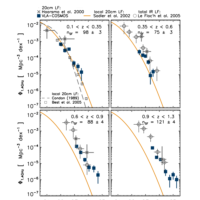
Figure 1.— 1.4 GHz luminosity functions (LFs) for star forming galaxies in the VLA-COSMOS survey, shown for four redshift ranges (filled blue squares) are presented in each panel. The number of galaxies in each redshift bin, statistically corrected for selection uncertainties (see text for details), is also indicated in each panel. The local 20 cm LFs for star forming galaxies are shown in the top-left panel (Condon 1989; Sadler et al. 2002; Best et al. 2005; the Sadler et al. 2002 LF – solid orange curve – is shown in all panels). In all panels we show the volume densities derived by Haarsma et al. (2000, gray asterisk), corrected to the current cosmology. In the top right, and bottom panels, the total IR LFs (Le Floc’h et al., 2005) for the corresponding redshift ranges (open circles) is also shown (see text for details). The total IR luminosity was converted to 1.4 GHz luminosity using the correlation given in Bell (2003).

In all panels we show the volume densities of 20 cm radio sources derived by Haarsma et al. (2000, gray asterisk), corrected to the current cosmology. Haarsma et al. used 37 star forming galaxies to derive these LFs (38% of these had approximate redshifts derived from I- or HK’- band magnitudes, the others had spectroscopic redshifts). Their data points in each redshift range agree fairly well within the error-bars with our results. Note that due to the almost one order of magnitude larger sample of star forming galaxies used here, the error-bars of the VLA-COSMOS LFs are significantly smaller.

In the higher redshift panels we also compare our LFs with the total IR LFs derived by Le Floc’h et al. (2005, hereafter LF05) based on a 24 $\mathrm{\mu m}$ selected sample in the CDFS (Chandra Deep Field South; top right and both bottom panels in Fig. 1). The total IR luminosity was converted to 1.4 GHz luminosity using the total IR – radio correlation (Bell, 2003), which has an intrinsic scatter of $\sim 0.26$ dex, shown by horizontal error bars in Fig. 1. The IR LFs were re-scaled to our redshift ranges either by combining two narrower redshift bins given in LF05 or by scaling a given comoving density using the evolution parameters, and their corresponding errors, given in LF05. There is an excellent agreement between the 1.4 GHz and IR LFs. Note also that the VLA-COSMOS LFs constrain much better than the IR data the high-luminosity end, i.e. the most intensely star-forming galaxies. Interestingly, the VLA-COSMOS star forming galaxies in our two highest redshift bins ($z>0.6$) show an extended high-luminosity ($\mathrm{L}_{1.4}$ $\gtrsim 2\times 10^{24}$ W Hz^-1) tail. We cannot exclude some possible contamination from AGN, which are much more numerous than SF galaxies at these high radio luminosities (see Fig. 17 in S08). However, a similar excess of SF galaxy volume densities at the high luminosity end has been recently found by Cowie et al. (2004), who have used the HDF-N and SSA 13 fields to derive the radio LF for spectroscopically identified SF galaxies (106 SF galaxies, $z\leq 1.4$).

2.4. Towards the derivation of the cosmic star formation history

The comparison of our derived LFs (see Fig. 1) with the local 20 cm LF shows a strong evolution with look-back time. The evolution of a given population of objects is usually parameterized with monotonic density and luminosity evolution. However, as the VLA-COSMOS data do not allow the derivation of the LF out to, and fainter than the characteristic luminosity (i.e. the ’knee’ of the LF), a full determination of the evolution is not possible with these data, and we choose to parameterize it using pure luminosity evolution. However, as we show below, its quantization depends fairly strongly on the choice of the local LF, as those presented in the literature are not exactly the same.

2.4.1 The local 20 cm luminosity functions

The two commonly used analytical forms for the local 20 cm radio LFs have been presented in Condon (1989) and Sadler et al. (2002). Condon et al. use a hyperbolic parameterization (see also Condon et al. 2002) of the form:

$$\log\Phi_{\mathrm{1.4GHz}} = 28.83-\frac{3}{2}\log L_{\mathrm{1.4GHz}}+Y$$ (2)

$$-\left[B^{2}+\frac{\left(\log L_{\mathrm{1.4GHz}}-X\right)^{2}}{W^{2}}\right]^{1/2}$$

where $Y=2.88$, $B=1.5$, $X=22.108$, $W=0.667$ (corrected to the current cosmology and the base of $d\log L$, compared to $d\,\mathrm{mag}$ given in Condon 1989). These parameters have been derived using a sample of 307 spiral and irregular galaxies from the Revised Shapley-Ames Catalog (RSA; Sandage et al., 1981) observed at 1.49 GHz (Condon, 1987, see Fig. 2).

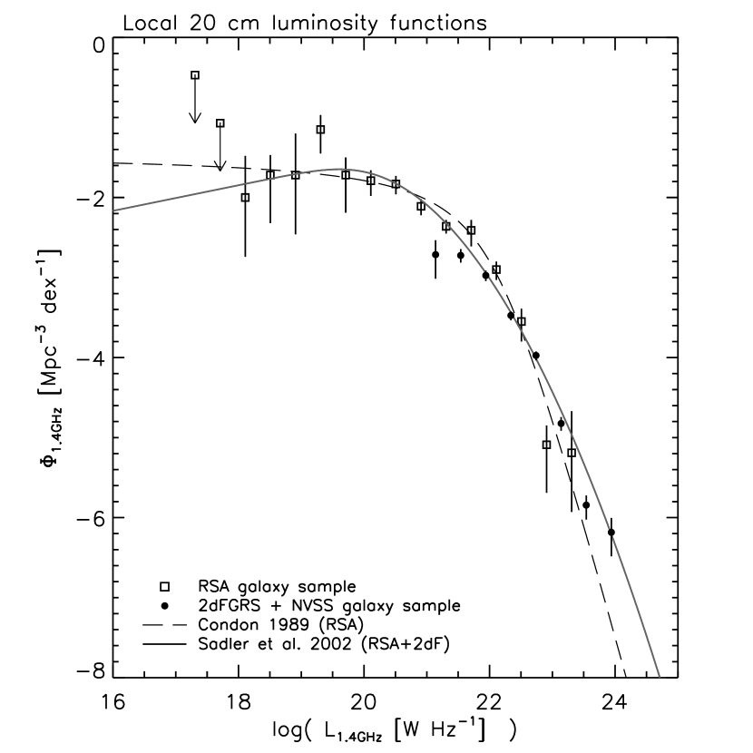
Figure 2.— Illustration of the differences in the shapes of the local 1.4 GHz radio luminosity functions (LFs) found in the literature (Condon, 1989; Sadler et al., 2002, corrected to the current cosmology). Also shown are the data points used for the analytical fits in Condon (1989, Revised-Shapley-Ames Catalogue; RSA) and Sadler et al. (2002, NVSS/2dFGRS and RSA samples). Note that the major difference in the representation of the local radio LFs is the analytical form used to fit the data (see eqs. 2 & 3) that particularly affects the position of the LF break (i.e. ’knee’).

The LF given in Sadler et al. (2002) takes on the form of a combined power-law and Gaussian distribution given by the following analytic function (first proposed by Sandage et al. 1979):

$$\Phi(L)=\Phi^{*}\left[\frac{L}{L_{*}}\right]^{1-\alpha}\exp{\left\{-\frac{1}{2\sigma^{2}}\left[\log{(1+\frac{L}{L_{*}})}\right]^{2}\right\}}$$ (3)

with $\alpha=0.84$, $\sigma=0.94$, $\Phi^{*}=22.9\times 10^{-3}$ Mpc^-3, and $L^{*}=1.95\times 10^{19}$ W Hz^-1 (scaled to the cosmology used here, and to the base of $d\log L$; see Hopkins 2004). Sadler et al. (2002) have used 204 SF galaxies drawn from the Two Degree Field Galaxy Redshift Survey (2dFGRS) and the 1.4 GHz NRAO VLA Sky Survey (NVSS) to derive their LF (see Fig. 2). However, to obtain the best fit parameters to eq. 3, they combined this sample (that constrains well the high luminosity end of the LF; see Fig. 2) with the RSA galaxy sample (in order to sample the low luminosity end of the LF).

The differences between the two local LFs are illustrated in Fig. 2. There is a discrepancy between the two analytical representations of the radio LFs at both the high and low luminosity ends. However, the discrepancy affecting most severely the star formation rate density, that we aim to derive here, is the different position of the LF’s turn-over point ($L_{*}$) given by the two analytic forms. This yields a difference of 10-50% in the star formation rate density integral (see e.g. Fig. 3 and Fig. 5) as the luminosity range encompassing the turn-over point ($10^{19}\lesssim L_{\mathrm{1.4GHz}}\lesssim 10^{23}$ W Hz^-1) contributes the most ($\sim 95\%$) to the integral. It is important to note that the 2dFGRS and NVSS data used by Sadler et al. (2002) sample more precisely the high-luminosity end (see Fig. 2) of the local radio LF when compared to the RSA sample (Condon, 1989). Hence, in Sec. 3.2 we will use the former one to constrain the evolution of our most intensely SF galaxies (i.e. $L_{1.4}\gtrsim 2.34\times 10^{23}$ W Hz^-1). As the total star formation rate density in each redshift range is derived by integrating under the evolved LF curve (multiplied with star formation rate; see below) down to the faintest 1.4 GHz luminosities, we will take this difference of the local 20 cm LFs into account in further analysis.

2.5. The evolution of star forming galaxies

We parameterize the evolution of the VLA-COSMOS SF galaxy LF by pure luminosity evolution:

$$\Phi_{z}(L)=\Phi_{z=0}\left[\frac{L}{(1+z)^{\alpha_{L}}}\right]$$ (4)

where $\alpha_{L}$ is the characteristic luminosity evolution parameter, and $\Phi_{z}$ is the luminosity function at redshift $z$. We derive the evolution by summing the $\chi^{2}$ distributions obtained for a large range of fixed $\alpha_{L}$ in each redshift bin (excluding our first – local – redshift bin). The uncertainty in $\alpha_{L}$ is then taken to be the $2\sigma$ error obtained from the $\chi^{2}$ statistics. Our results yield a pure luminosity evolution with i) $\alpha_{L}=2.1\pm 0.2$, when the Sadler et al. (2002) local LF is used, and ii) $\alpha_{L}=2.5\pm 0.1$ when the Condon (1989) local LF is used. The different evolution parameters are a natural consequence of the different slopes of the two local LFs in the luminosity range that is constrained by the VLA-COSMOS data (see Figs. 2 and 3).

Haarsma et al. (2000) have found that a pure luminosity evolution with $\alpha_{L}\approx 2.74$ is a good representation of the evolution of their radio-selected SF galaxies [no uncertainties were associated with this estimate]. They used the Condon (1989) local LF as the basis for deriving their evolution. Given i) their much smaller sample size, and ii) that their LF, when corrected for cosmology, agrees well with the one derived here (see Fig. 1), these two results are in good agreement. Further, Cowie et al. (2004) find an evolution of the SF galaxy LF (using the Condon 1989 local LF) consistent with $\alpha_{L}$ of 3. The SF LFs, as well as the evolution, derived here agree with their findings (c.f. Fig 3 in Cowie et al. 2004). Our results are also consistent with the overall evolution of star forming galaxies obtained by Hopkins (2004, $\alpha_{L}=2.7\pm 0.6$), that has been shown to fit well the evolution of radio selected star forming galaxies at low redshifts ($z\leq 0.5$; Afonso et al., 2005, Phoenix Deep Survey).

3. The cosmic star formation history (CSFH)

3.1. The total cosmic star formation history

Figure 3.— Luminosity density for VLA-COSMOS star forming galaxies (filled squares) in 4 redshift bins. The solid and dashed curves correspond to the best fit LFs in each redshift bin using the local LF given in Sadler et al. (2002) and Condon (1989), respectively. Note that the first appears to describe the bright-luminosity end more consistently with our data.

As the star formation rate density (SFRD) is derived by integrating the luminosity density, in Fig. 3 we show the luminosity density for our 4 redshift bins. The shown curves are the two local 20 cm LFs (Condon, 1989; Sadler et al., 2002), purely evolved in luminosity, and best fit to the VLA-COSMOS data in each redshift range. Prior to integration, we convert the 1.4 GHz radio luminosity to star formation rates ($\psi$, in $\mathrm{M}_{\odot}\,\mathrm{yr}^{-1}$), using the calibration given in Bell (2003), based on the total IR – radio correlation:

$$\mathrm{\psi\,\,[\mathrm{M}_{\odot}\,\mathrm{yr}^{-1}]}=\left\{\begin{array}[]{lr}5.52\times 10^{-22}\,\,\mathrm{L_{1.4}}\,\,,&\mathrm{L_{1.4}}>\mathrm{L_{c}}\\ \frac{5.52\times 10^{-22}}{0.1+0.9\left(\mathrm{L_{1.4}}/L_{c}\right)^{0.3}}\,\,\mathrm{L_{1.4}}\,\,,&\mathrm{L_{1.4}}\leq\mathrm{L_{c}}\end{array}\right.$$ (5)

where $\mathrm{L_{c}}=6.4\times 10^{21}$ W Hz^-1, and $\mathrm{L_{1.4}}$ is the 1.4 GHz radio luminosity in units of W Hz^-1. This calibration uses a Salpeter initial mass function (IMF $\propto M^{-2.35}$) from 0.1 – 100 $\mathrm{M}_{\odot}$. After the conversion, we compute the star formation rate density (SFRD) for a given redshift bin as $\int\psi\left(L\right)\,\Phi_{z}\left(L\right)\,dL$, where $\Phi_{z}$ is the evolved radio LF best fit to the data in each redshift range (see curves in Fig. 3).

In Fig. 4 we first show the SFRD, obtained by numerically integrating the VLA-COSMOS data (open squares) within the sampled luminosity range, with no attempt made to extrapolate towards the faint or bright luminosity ends using the evolved local LF. This eliminates any assumption, and yields robust lower limits purely obtained from the data. The dependence of the derived SFRD on the faint/bright end extrapolation is illustrated by the (solid and dashed) curves in Fig. 4, which were obtained using the average pure luminosity evolution of the two local LFs derived in Sec. 2.5, and integrating over the entire SFRD curve. Hence, the largest uncertainty in the derivation of the SFRD based on radio data arises from the uncertainty in the shape of the local radio LF (assumed not to change with redshift), and the associated extrapolation below the faintest luminosity sampled by the data.

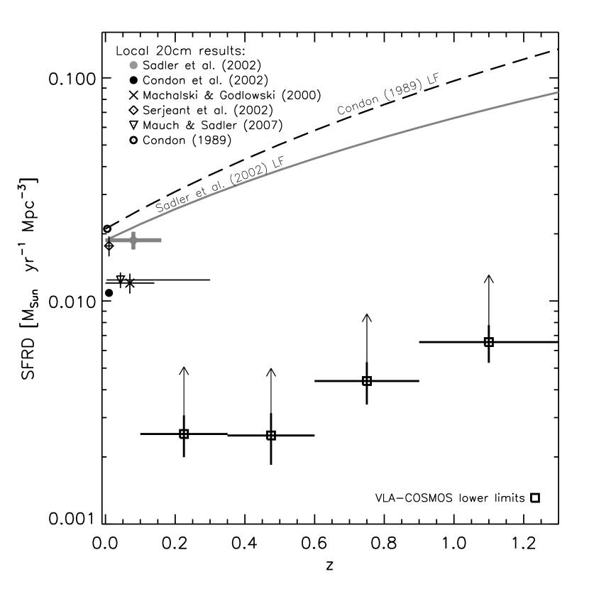
Figure 4.— Star formation rate density (SFRD) as a function of redshift. Open squares represent the SFRD derived from pure VLA-COSMOS data, without any extrapolations towards the faint or bright luminosity end. Therefore, they present strict lower limits, and are indicated with arrows. The two curves shown correspond to the average evolution of the VLA-COSMOS SF galaxies derived using two different local radio LFs (Condon, 1989; Sadler et al., 2002). Local SFRDs derived by various authors are also shown, and indicated in the panel.

Table 1 1.4 GHz radio luminosity functions for VLA-COSMOS star forming galaxies ($H_{0}=70,\,\Omega_{M}=0.3,\Omega_{\Lambda}=0.7$).

redshift	$\mathrm{L_{1.4GHz}}$	$\Phi$
range	$[\mathrm{WHz^{-1}}]$	$[\mathrm{Mpc^{-3}dex^{-1}]}$
	$1.0\cdot 10^{22}$	$7.0\pm 1.5\cdot 10^{-4}$
$0.1<z\leq 0.35$	$2.0\cdot 10^{22}$	$2.9\pm 0.7\cdot 10^{-4}$
	$4.0\cdot 10^{22}$	$3.5\pm 0.6\cdot 10^{-4}$
	$8.9\cdot 10^{22}$	$5.0\pm 2.1\cdot 10^{-5}$
	$1.8\cdot 10^{23}$	$3.2\pm 1.6\cdot 10^{-5}$
	$3.2\cdot 10^{23}$	$1.4\pm 1.0\cdot 10^{-5}$
	$3.5\cdot 10^{22}$	$2.4\pm 0.9\cdot 10^{-4}$
$0.35<z\leq 0.6$	$6.3\cdot 10^{22}$	$1.5\pm 0.4\cdot 10^{-4}$
	$1.0\cdot 10^{23}$	$1.3\pm 0.3\cdot 10^{-4}$
	$1.6\cdot 10^{23}$	$5.8\pm 1.6\cdot 10^{-5}$
	$2.2\cdot 10^{23}$	$9.0\pm 6.4\cdot 10^{-6}$
	$3.5\cdot 10^{23}$	$1.5\pm 0.7\cdot 10^{-6}$
	$1.4\cdot 10^{23}$	$1.2\pm 0.2\cdot 10^{-5}$
$0.6<z\leq 0.9$	$2.8\cdot 10^{23}$	$4.8\pm 0.9\cdot 10^{-5}$
	$5.6\cdot 10^{23}$	$1.7\pm 0.5\cdot 10^{-5}$
	$1.1\cdot 10^{24}$	$5.8\pm 2.6\cdot 10^{-6}$
	$2.5\cdot 10^{24}$	$5.2\pm 2.3\cdot 10^{-6}$
	$5.0\cdot 10^{24}$	$2.0\pm 1.4\cdot 10^{-6}$
	$3.2\cdot 10^{23}$	$9.2\pm 1.5\cdot 10^{-5}$
$0.9<z\leq 1.3$	$6.3\cdot 10^{23}$	$2.4\pm 0.5\cdot 10^{-5}$
	$1.3\cdot 10^{24}$	$1.8\pm 0.4\cdot 10^{-5}$
	$2.8\cdot 10^{24}$	$3.2\pm 1.4\cdot 10^{-6}$
	$5.6\cdot 10^{24}$	$1.2\pm 0.8\cdot 10^{-6}$
	$1.0\cdot 10^{25}$	$2.0\pm 1.0\cdot 10^{-6}$
	$1.8\cdot 10^{25}$	$1.0\pm 0.7\cdot 10^{-6}$

We compare our SFRD results (given in Tab. 2), obtained by integrating over the best fit evolved local LF in each redshift range (see curves in Fig. 3), with other radio-based estimates in Fig. 5. The expected steep decline in the star formation rate density since $z\sim 1$ is reproduced by our data. Our results are consistent within the errors with the results from Haarsma et al. (2000, who used the local LF), although their results are on average higher. Note also that our statistical CSFH uncertainties (bold red crosses in Fig. 5) are significantly smaller compared to the Haarsma et al. (2000) results, as a result of the larger sample utilized here. Our results are also qualitatively consistent with those obtained by Ivison et al. (2007), based on radio image stacking of UV selected galaxies in the AEGIS20 survey.

Table 2 Star formation rate density (derived using the calibration given in Bell 2003; see eq. 5) from 1.4 GHz VLA-COSMOS data ($H_{0}=70,\,\Omega_{M}=0.3,\Omega_{\Lambda}=0.7$).

redshift	SFRD	[$\mathrm{M}_{\odot}\,\mathrm{yr}^{-1}$]
range	Condon (1989) LF	Sadler et al. (2002) LF
$0.1<z\leq 0.35$	$0.025^{+0.001}_{-0.001}$	$0.023^{+0.002}_{-0.002}$
$0.35<z\leq 0.6$	$0.043^{+0.003}_{-0.003}$	$0.032^{+0.003}_{-0.002}$
$0.6<z\leq 0.9$	$0.067^{+0.003}_{-0.003}$	$0.048^{+0.003}_{-0.004}$
$0.9<z\leq 1.3$	$0.134^{+0.010}_{-0.009}$	$0.088^{+0.005}_{-0.005}$

Seymour et al. (2008) have used VLA/MERLIN radio frequency observations of the 13^H XMM-Newton/Chandra Deep field to derive the cosmic star formation history. Their findings are qualitatively consistent with those from Haarsma et al. (2000, shown in Fig. 5) when they use the Mauch & Sadler (2007) local LF evolved in luminosity with an a-priori set value of $\alpha_{L}=2.5$ (note that this local LF has a lower normalization than Sadler et al. 2002; see the local results in Fig. 4 and Fig. 5). Further, they used a different radio luminosity to SFR relation that is consistent with 0.84 times the Bell (2003) calibration used here (see Seymour et al. 2008 for details). Hence, this implies that their results are significantly higher than the VLA-COSMOS results. Further, given the differences between the local radio LFs outlined in Sec. 2.4.1, if Seymour et al. (2008) had chosen to use the Condon (1989) local LF with otherwise the same assumptions, they would have obtained even higher SFRD values. We believe that the main reason for the differences between our results and those by Seymour et al. (2008) is likely a combination of i) their a-priori assumed evolution of the local LF, contrary to constraining the evolution by their data and ii) the inclusion of a fraction of lower power (i.e. radio quiet) AGN in their star forming galaxy sample, while our sample may over-subtract composite objects (see also Sec. 4).

In Fig. 6 we compare the VLA-COSMOS derived CSFH data with results from previous studies based on a range of SF estimators – UV, optical, FIR, total IR, and radio. A luminosity-dependent obscuration correction was used where necessary (see Hopkins 2004, and references therein). Overall, our derived CSFH agrees with the general trend of a rapid decline by almost an order of magnitude in the cosmic star formation rate density since $z\sim 1$. A possibly slower decline is suggested by our data if the Sadler et al. (2002) LF is used. However, as the uncertainties due to the faint-end extrapolation are significant, no robust conclusions can be made at this point.

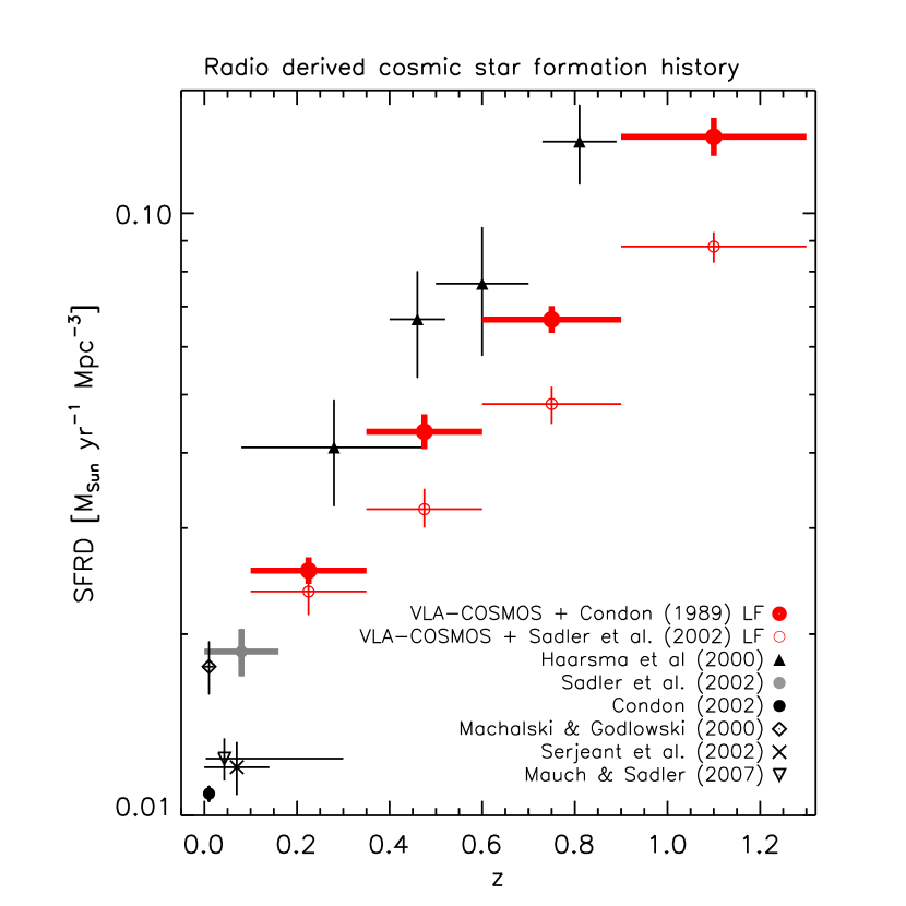
Figure 5.— Comparison of radio derived cosmic star formation histories. The different samples are indicated in the panel. The bold red circles show the VLA-COSMOS results, when the Condon (1989) local LF is used; open red circles show the results when the Sadler et al. (2002) local LF is used. Results based on other radio-based studies are also shown, and indicated in the panel.

3.2. The CSFH of intensely star forming galaxies

The VLA-COSMOS SF galaxy sample constrains well the high end of the LF for SF galaxies. Given the 2$\Box^{\circ}$ VLA-COSMOS field the comoving volume sampled up to $z=1.3$ is $\sim 1.3\times 10^{7}$ Mpc³, corresponding roughly to the volume observed locally by SDSS (DR1). Thus, for the first time this allows a robust derivation of the CSFH for galaxies forming stars at rates of $\gtrsim 100$ $\mathrm{M}_{\odot}\,\mathrm{yr}^{-1}$ out to $z=1.3$. Such radio selected galaxies are equivalents to the ultra-luminous IR galaxies (ULIRGs, $\mathrm{L_{IR}}>10^{12}$ $\mathrm{L}_{\odot}$), and it is noteworthy that the VLA-COSMOS survey is sensitive to a complete sample of these galaxies out to $z\sim 1$ (see Fig. 16 in S08).

In order to derive the evolution of the SFRD at the high-luminosity end, we integrate the SFRD curve, obtained from the best fit pure radio luminosity evolution in each redshift bin (see Fig. 3), only for our SF galaxies that have $L_{1.4}\gtrsim 2.34\times 10^{23}$ W Hz^-1, which corresponds to $\mathrm{L_{IR}}>10^{12}$ $\mathrm{L}_{\odot}$ given the adopted total IR – radio correlation (Bell, 2003). For this we use the local LF given by Sadler et al. (2002) as it appears to be better suited for the high-luminosity end compared to the Condon (1989) LF (see Fig. 2). Note that for these highly luminous galaxies the extrapolation uncertainties are not as significant as for the overall SFRD, as this sample is almost complete in all three high redshift ranges. A small extrapolation to the faint end, given the form of the evolved local LF, is necessary only in the last redshift bin. For a consistent comparison between our radio and IR (LF05) results we convert the total IR luminosity to star formation rates consistently using the calibration given by Bell (2003). The results are shown in Fig. 7. The evolution of our star forming ULIRGs is consistent with the lower envelope derived by LF05. However, it is marginally flatter, suggesting a slower evolution of star forming ULIRG galaxies since $z=1.3$. This will be further discussed in the next section.

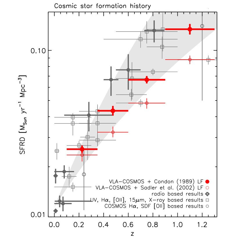
Figure 6.— Comparison of the VLA-COSMOS derived cosmic star formation history (red symbols; see Fig. 5 for details) with other-wavelength based results. The compilation of CSFHs contains UV-, H$\alpha-$, FIR-, and X-ray- based results, corrected for dust-obscuration using luminosity-dependent corrections (open gray squares; see Hopkins 2004 for details). Thick gray diamonds denote local radio estimates (Machalski & Godlowski 2000; Condon et al. 2002; Sadler et al. 2002; Serjeant et al. 2002). For all radio data the 1.4 GHz luminosity to star formation rate calibration given in Bell (2003, see eq. 5) is used. The gray-shaded area shows the cosmic star formation history derived by LF05, based on 24 $\mathrm{\mu m}$ data. The open gray circles denote i) the H$\alpha$ derived SFRD at $z=0.24$ in the COSMOS field, corrected for both dust-obscuration and AGN contribution (Shioya et al., 2008), and ii) the dust-obscuration corrected SFRD at $z=1.2$ derived using [OII] emission galaxies in the Subaru Deep Field (SDF; see for Takahashi et al. 2007 details).

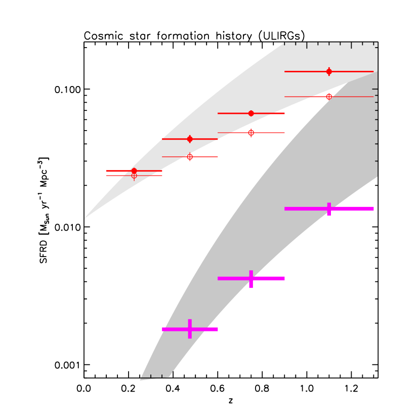
Figure 7.— Cosmic star formation history (CSFH) derived from VLA-COSMOS data for the overall population (red symbols as in Fig. 6), and only for star forming ULIRGs (magenta symbols; derived using the Sadler et al. 2002 local LF evolved in luminosity in each redshift bin). Also shown is the CSFH for the entire (light-gray shaded curve), and the ULIRG population (dark-gray shaded curve), derived from the evolved total IR luminosity function (LF05). The IR- and radio- based star formation rates have been put on the same relative scale (see text for details). Note that the VLA-COSMOS data suggest a slightly slower evolution of the star forming ULIRG population with redshift.

4. Discussion

4.1. The evolution of the most intensely star forming galaxies

Making use of our large statistical sample of radio-selected star forming ULIRGs complete out to $z\sim 1$ we have derived the CSFH of the most intensely star forming galaxies ($\gtrsim 100$ $\mathrm{M}_{\odot}$ yr^-1) out to $z=1.3$. Our evolution of the cosmic star formation rate in star forming ULIRGs qualitatively agrees with previous MIR-based results (LF05; see Fig. 7). However, we find a slightly slower evolution than predicted by the MIR results. The major cause for this difference is currently unclear, nonetheless there are likely three effects that may contribute:

i) No attempt has been made to minimize the AGN contamination in the 24 $\mathrm{\mu m}$- selected sample possibly causing an overestimate in the MIR-derived SFRD evolution for ULIRGs. For example, Caputi et al. (2007) have found $>10\%$ of 24 $\mathrm{\mu m}$-AGN at $z\sim 1$, and a factor of 2 more at $z\sim 2$, suggesting that the AGN fraction in MIR selected samples increases with redshift. The AGN fraction in MIR samples may also be a function of stellar mass. Although at higher redshift than analyzed here (implying a different cosmological era), Daddi et al. (2007) have demonstrated that at $z\sim 2$ the MIR AGN fraction is indeed a function of stellar mass, and reaches $\sim 50-60\%$ for masses $>4\times 10^{10}$ $\mathrm{M}_{\odot}$. The median stellar mass of the VLA-COSMOS star forming galaxies (obtained via SED fitting; see S08 for details) is $\sim 7\times 10^{10}$ $\mathrm{M}_{\odot}$.

ii) Particular care was taken to separate the VLA-COSMOS population into SF and AGN galaxies. Nonetheless, it has to be noted that some uncertainty, due to AGN contamination as well as incompleteness of the star forming galaxy sample exists, especially on the galaxy-by-galaxy and composite (SF plus AGN) galaxy level (see Smolčić et al. 2008 for details). It is also worth noting that two significant large scale structure components exist in our highest redshift bin (Scoville et al. 2007a, Scoville et al., in prep) that may affect the fraction of SF and AGN galaxies present in this particular redshift range.

iii) The local IRAS total IR and the Sadler et al. radio LFs, used for the derivation of these results, are not perfectly similar. There may also be a volume density excess of SF galaxies with high radio luminosities at $z>0.6$, compared to the Sadler et al. LF evolved only in luminosity. In addition, the total IR – radio correlation, used to select ULIRGs from our radio sample, carries its own uncertainty and intrinsic astrophysical scatter (Bressan et al., 2002; Bell, 2003). Therefore, it is not immediately obvious whether the same results would be expected based on both – radio and MIR – star formation indicators.

In summary, it is encouraging that the same qualitative behavior of the evolution of the ULIRG population is observed with the two independent, radio and MIR, SFR indicators. However, further dedicated studies of the details will prove most interesting in understanding the quantitative differences seen in Fig. 7.

4.2. The rapid decline of the CSFH since $z\sim 1$

Our overall CSFH (Fig. 6) agrees well with past findings, when these are corrected for dust-obscuration as needed. This verifies the assumptions about large dust-obscuration corrections required, especially for short-wavelength (e.g. UV) star formation tracers. Our radio data independently confirm the $\sim 1$ order of magnitude decline in the cosmic star formation rate since $z\sim 1$.

Based on UV and IR based SFR/morphology studies (Wolf et al., 2005; Bell et al., 2005; Melbourne et al., 2005; Hammer et al., 2005; Zamojski et al., 2007) this rapid decline in the overall cosmic star formation history is expected to be driven by normal spiral galaxies. For example, Bell et al. (2005) have performed a detailed morphological study of a galaxy sample ($z=0.7$) with SFRs $\gtrsim 10$ $\mathrm{M}_{\odot}\,\mathrm{yr}^{-1}$. They have demonstrated that physical processes that do not substantially affect galaxy morphology, such as minor mergers, gas consumption and weak interactions with satellite galaxies, may be most important for the rapid decline in the overall CSFH (see also e.g.  Somerville et al., 2001).

The sample analyzed here, however, is most sensitive to ULIRGs (SFR $\gtrsim 100$ $\mathrm{M}_{\odot}\,\mathrm{yr}^{-1}$), and those are the systems a priori expected to be a reflection of galaxy merging (based on local ULIRG morphology studies; Sanders & Mirabel, 1996). This implies that the rapid decline in CSFH of our ULIRGs (Fig. 7) may be more affected by galaxy mergers than the overall CSFH decline since $z\sim 1$. Intriguingly, our derived LF evolution is very similar to the evolution of the galaxy close-pair fraction, derived for bright galaxies ($>L_{V}^{*}$; Kartaltepe et al., 2007) in the COSMOS field, well described with a power law with an index of $3.1\pm 0.1$ (or $2.2\pm 0.1$ when pure luminosity evolution is considered; see also e.g. Lotz et al. 2008). This strong evolution of the bright close-pair fraction, combined with a similarly strong evolution of the CSFH of ULIRGs derived here suggests that major mergers may play an important role in the rapid decline of the CSFH since $z\sim 1$ for the most intensely star forming galaxies. Thus, the observed steep evolution of our ULIRG population may be a good record of merger rate evolution, combined with gas content evolution.

5. Summary

We have derived the cosmic star formation history out to $z=1.3$ using to date the largest sample of radio-selected star forming galaxies observed at 1.4 GHz (20 cm) in the VLA-COSMOS survey. The large increase in the number of radio selected SF galaxies out to high redshift, compared to previous studies, allowed us to constrain well the evolution of the 1.4 GHz luminosity function for radio-selected star forming galaxies, as well as to reduce significantly the statistical uncertainties of the radio-derived CSFH. We find that the uncertainties are ruled by the differences in the shape of the local radio LFs present in the literature. A pure radio luminosity evolution of VLA-COSMOS star forming galaxies is well described with $L_{*}\propto(1+z)^{2.1\pm 0.2}$, when evolving the Sadler et al. (2002) local LF, or with $L_{*}\propto(1+z)^{2.5\pm 0.1}$ when evolving the Condon (1989) local LF. Although encompassing a relatively broad range, both values are consistent with previously derived evolution of star forming galaxies (e.g. Condon et al. 2002; Hopkins 2004; Cowie et al. 2004; Afonso et al. 2005).

Our overall CSFH agrees well with past findings, when these are corrected for dust-obscuration where needed. This verifies the assumptions about large dust-obscuration corrections required, especially for short-wavelength (e.g. UV) star formation tracers. Making use of our large statistical sample of radio-selected star forming ULIRGs complete out to $z\sim 1$ we have robustly constrained the high-end of the SF galaxy LF at different cosmic times. Using these we have derived the CSFH of the most intensely star forming galaxies ($\gtrsim 100$ $\mathrm{M}_{\odot}$ yr^-1; i.e. star forming ULIRGs) out to $z=1.3$. We find an, on average, slower evolution of the cosmic star formation rate in star forming ULIRGs than predicted by MIR results consistent with the fraction of star forming galaxies in MIR samples likely becoming lower with increasing redshift and/or stellar mass.

References

- Afonso et al. (2005) Afonso, J., Georgakakis, A., Almeida, C., Hopkins, A. M., Cram, L. E., Mobasher, B., & Sullivan, M. 2005, ApJ, 624, 135
- Barger et al. (2007) Barger, A. J., Cowie, L. L., & Wang, W.-H. 2007, ApJ, 654, 764
- Bell (2003) Bell, E. F. 2003, ApJ, 586, 794
- Bell et al. (2005) Bell, E. F., et al. 2005, ApJ, 625, 23
- Bell et al. (2007) Bell, E. F., Zheng, X. Z., Papovich, C., Borch, A., Wolf, C., & Meisenheimer, K. 2007, ApJ, 663, 834
- Best et al. (2005) Best, P. N., et al. 2005, MNRAS, 362, 9
- Bondi et al. (2008) Bondi, M., Ciliegi, P., Schinnerer, E., Smolčić, V., Jahnke, K., Carilli, C., & Zamorani, G. 2008, ApJ, 681, 1129
- Bressan et al. (2002) Bressan, A., Silva, L., & Granato, G. L. 2002, A&A, 392, 377
- Caputi et al. (2007) Caputi, K. I., et al. 2007, ApJ, 660, 97
- Condon (1987) Condon, J. J. 1987, ApJS, 65, 485
- Condon (1989) Condon, J. J. 1989, ApJ, 338, 13
- Condon (1992) Condon, J. J. 1992, ARA&A, 30, 575
- Condon et al. (2002) Condon, J. J., Cotton, W. D., & Broderick, J. J. 2002, AJ, 124, 675
- Cooper et al. (2008) Cooper, M. C., et al. 2008, MNRAS, 383, 1058
- Cowie et al. (2004) Cowie, L. L., Barger, A. J., Fomalont, E. B., & Capak, P. 2004, ApJ, 603, L69
- Cucciati et al. (2006) Cucciati, O., et al. 2006, A&A, 458, 39
- Daddi et al. (2007) Daddi, E., et al. 2007, ArXiv e-prints, 705, arXiv:0705.2832
- Dressler (1980) Dressler, A. 1980, ApJ, 236, 351
- Elbaz et al. (2007) Elbaz, D., et al. 2007, A&A, 468, 33
- Fomalont et al. (1991) Fomalont, E. B., Windhorst, R. A., Kristian, J. A., & Kellerman, K. I. 1991, AJ, 102, 1258
- Haarsma et al. (2000) Haarsma, D. B., et al. 2000, ApJ, 544, 641
- Hammer et al. (1995) Hammer, F., Crampton, D., Lilly, S. J., Le Fevre, O., & Kenet, T. 1995, MNRAS, 276, 1085
- Hammer et al. (2005) Hammer, F., Flores, H., Elbaz, D., Zheng, X. Z., Liang, Y. C., & Cesarsky, C. 2005, A&A, 430, 115
- Hopkins (2004) Hopkins, A. M. 2004, ApJ, 615, 209
- Huynh et al. (2008) Huynh, M. T., Jackson, C. A., Norris, R. P., & Fernandez-Soto, A. 2008, AJ, 135, 2470
- Ivison et al. (2007) Ivison, R. J., et al. 2007, ApJ, 660, L77
- Le Floc’h et al. (2005) Le Floc’h, E., et al. 2005, ApJ, 632, 169
- Kartaltepe et al. (2007) Kartaltepe, J. S., et al. 2007, ApJS, 172, 320
- Lotz et al. (2008) Lotz, J. M., et al. 2008, ApJ, 672, 177
- Machalski & Godlowski (2000) Machalski, J., & Godlowski, W. 2000, A&A, 360, 463
- Mauch & Sadler (2007) Mauch, T., & Sadler, E. M. 2007, MNRAS, 375, 931
- Melbourne et al. (2005) Melbourne, J., Koo, D. C., & Le Floc’h, E. 2005, ApJ, 632, L65
- McCracken et al. (2007) McCracken, H. J., et al. 2007, ApJS, 172, 314
- Richards et al. (1998) Richards, E. A., Kellermann, K. I., Fomalont, E. B., Windhorst, R. A., & Partridge, R. B. 1998, AJ, 116, 1039
- Sadler et al. (2002) Sadler, E. M., et al. 2002, MNRAS, 329, 227
- Sandage et al. (1979) Sandage, A., Tammann, G. A., & Yahil, A. 1979, ApJ, 232, 352
- Sandage et al. (1981)
- Sanders & Mirabel (1996) Sanders, D. B., & Mirabel, I. F. 1996, ARA&A, 34, 749
- Schinnerer et al. (2007) Schinnerer, E., et al. 2007, ApJS, 172, 46
- Schmidt (1968) Schmidt, M. 1968, ApJ, 151, 393
- Scoville et al. (2007a) Scoville, N., et al. 2007a, ApJS, 172, 1
- Scoville et al. (2007b) Scoville, N., et al. 2007b, ApJS, 172, 150
- Serjeant et al. (2002) Serjeant, S., Gruppioni, C., & Oliver, S. 2002, MNRAS, 330, 621
- Seymour et al. (2008) Seymour, N., et al. 2008, MNRAS, 386, 1695
- Shioya et al. (2008) Shioya, Y., et al. 2008, ApJS, 175, 128
- Smolčić et al. (2006) Smolčić, V., et al. 2006, MNRAS, 371, 121
- Smolčić et al. (2008) Smolčić, V., et al. 2008, ApJS, 177, 14
- Somerville et al. (2001) Somerville, R. S., Primack, J. R., & Faber, S. M. 2001, MNRAS, 320, 504
- Takahashi et al. (2007) Takahashi, M. I., et al. 2007, ApJS, 172, 456
- Windhorst et al. (1995) Windhorst, R. A., Fomalont, E. B., Kellermann, K. I., Partridge, R. B., Richards, E., Franklin, B. E., Pascarelle, S. M., & Griffiths, R. E. 1995, Nature, 375, 471
- Wolf et al. (2005) Wolf, C., et al. 2005, ApJ, 630, 771
- Zamojski et al. (2007) Zamojski, M. A., et al. 2007, ApJS, 172, 468
- Zheng et al. (2006) Zheng, X. Z., et al. 2006, ApJ, 640, 784
- Zheng et al. (2007) Zheng, X. Z., Bell, E. F., Papovich, C., Wolf, C., Meisenheimer, K., Rix, H.-W., Rieke, G. H., & Somerville, R. 2007, ApJ, 661, L41