Subaru and Keck Observations of
the Peculiar Type Ia Supernova 2006gz at Late Phases

Abstract

Recently, a few peculiar Type Ia supernovae (SNe) that show exceptionally large peak luminosity have been discovered. Their luminosity requires more than 1 M_⊙ of ⁵⁶Ni ejected during the explosion, suggesting that they might have originated from super-Chandrasekhar mass white dwarfs. However, the nature of these objects is not yet well understood. In particular, no data have been taken at late phases, about one year after the explosion. We report on Subaru and Keck optical spectroscopic and photometric observations of the SN Ia 2006gz, which had been classified as being one of these “overluminous” SNe Ia. The late-time behavior is distinctly different from that of normal SNe Ia, reinforcing the argument that SN 2006gz belongs to a different subclass than normal SNe Ia. However, the peculiar features found at late times are not readily connected to a large amount of ⁵⁶Ni; the SN is faint, and it lacks [Fe II] and [Fe III] emission. If the bulk of the radioactive energy escapes the SN ejecta as visual light, as is the case in normal SNe Ia, the mass of ⁵⁶Ni does not exceed $\sim 0.3$ M_⊙. We discuss several possibilities to remedy the problem. With the limited observations, however, we are unable to conclusively identify which process is responsible. An interesting possibility is that the bulk of the emission might be shifted to longer wavelengths, unlike the case in other SNe Ia, which might be related to dense C-rich regions as indicated by the early-phase data. Alternatively, it might be the case that SN 2006gz, though peculiar, was actually not substantially overluminous at early times.

1. INTRODUCTION

There is general agreement that Type Ia supernovae (SNe Ia) are thermonuclear explosions of white dwarfs (WDs; e.g., Nomoto, Iwamoto, & Kishimoto 1997; Hillebrandt & Niemeyer 2000). Thanks to the uniformity of their light-curve shapes after applying a correction factor (Phillips 1993; Phillips et al. 1999), they can be used as “standard candles” to measure cosmological parameters, which led to the discovery of the accelerating expansion of the universe and dark energy (Riess et al. 1998; Perlmutter et al. 1999; see Filippenko 2005 for a review). However, the nature of their progenitor systems has not been resolved (e.g., Livio 2000; Hillebrandt & Niemeyer 2000; Nomoto et al. 2003), making it difficult to reliably predict potential evolutionary effects that could add systematic errors to the determination of cosmological parameters.

The progenitors of normal SNe Ia (Branch, Fisher, & Nugent 1993; Li et al. 2001) are believed to be WDs having nearly the Chandrasekhar mass (hereafter Ch-SN Ia and Ch-WD). The recent discovery of extremely luminous SNe Ia raises the possibility that not all SNe Ia originate from a single type of progenitor system. Howell et al. (2006) reported that SN Ia 2003fg (SNLS-03D3bb) reached an absolute $V$-band magnitude of $M_{V}=-19.94$ ($H_{0}=70$ km s^-1 Mpc^-1, $\Omega_{\rm M}=0.3$, flat universe). Assuming that this luminosity is powered by the decay chain ⁵⁶Ni $\to$ ⁵⁶Co $\to$ ⁵⁶Fe as in other SNe Ia, they estimated $M_{\rm 56Ni}\approx 1.29$ M_⊙ (hereafter $M_{\rm 56Ni}$ is the mass of ⁵⁶Ni produced and ejected during the explosion). Combining this with other elements whose existence in the ejecta is evident from the spectra, the ejecta and progenitor masses should exceed the Chandrasekhar limit of a nonrotating WD. This was the first observationally based suggestion of an SN Ia from a super-Chandrasekhar WD (hereafter SupCh-SN Ia and SupCh-WD). Since then, two other possibly overluminous SNe Ia have been reported: SN 2006gz (Hicken et al. 2007) and SN 2007if (Yuan et al. 2007).

Table 1Spectroscopy ($+341$ days)

Filter	Wavelengths	Airmass	Exposure (s)
O58 + R300	5,800–10,200 Å	1.056	1200
None + B300	4,700–9,000 Å	1.085	1200
Y47 + B300	3,800–7,200 Å	1.165	1200

All of the available data for these SNe Ia are only for the early phases, $t\mathrel{\hbox to0.0pt{\lower 4.0pt\hbox{\hskip 1.0pt$\sim$}\hss}\raise 1.0pt\hbox{$<$}}100$ d (hereafter $t$ is the time since the explosion). At later times, SNe Ia enter the nebular phase, when the Fe-rich innermost ejecta, which are hidden at early phases, can be directly observed (e.g., Axelrod 1988). In this paper, we report late-time spectroscopy and photometry of the potentially overluminous SN 2006gz taken with the 8.2-m Subaru telescope and the 10-m Keck I telescope. In §2 we present the observations and data reduction. Results are shown in §4, along with some comparisons to model calculations (§3). SN 2006gz is intrinsically different from normal SNe Ia. However, our results are not readily interpretable in the SupCh-SN Ia scenario, raising questions about the nature of this new subclass of objects, as discussed in §5.

2. OBSERVATIONS AND DATA REDUCTION

Spectroscopy and imaging of SN 2006gz were performed on 2007 September 18 (UT dates are used throughout this paper) with the 8.2-m Subaru telescope equipped with the Faint Object Camera and Spectrograph (FOCAS; Kashikawa et al. 2002). The epoch corresponds to $t=t_{\rm peak}+341$ d, where $t_{\rm peak}$ is the time at $B$-band maximum (JD 2,454,020.2; Hicken et al. 2007) measured from the unknown explosion date. The field was also imaged on 2007 October 14 ($t=t_{\rm peak}+367$ d) with the $10$-m Keck I telescope equipped with the Low Resolution Imaging Spectrometer (LRIS; Oke et al. 1995). The seeing conditions were excellent on both nights; star profiles had full width at half-maximum intensity (FWHM) of $\sim 0\arcsec.8$ and $0\arcsec.7$, respectively. The same field was imaged again on 2007 November 6 by the Subaru/FOCAS ($t=t_{\rm peak}+390$ d), although the seeing was not good (FWHM $\approx 1\arcsec.5$).

For the Subaru spectroscopy on September 18, we took three spectra with exposure time 1200 s each. We used the $0\farcs 8$-wide slit and the R300 grism with the O58 filter (wavelength coverage 5800–10200 Å), the B300 grism with the Y47 filter (4700–9000 Å), and the B300 grism with no filter (3800–7200 Å), in the three separate exposures. The standard star G191B2B (Massey & Gronwall 1990) was also observed for flux calibration. Although the signal-to-noise ratio (S/N) is low, we succeeded in obtaining a spectrum of the SN (§3). The spectroscopic observations are summarized in Table 1.

Table 2Photometry

UT Date (2007)	Phase	Telescope	Exposure (s)	Band	Magnitude
September 18	+341	Subaru	60	$B$	$>24.4$
		Subaru	60	$V$	$>24.2$
		Subaru	60	$R$	$>24.0$
October 14	+367	Keck	555	$R$	$25.5\pm 0.3$
		Keck	645	$g$	$25.5\pm 0.2$
November 6	+390	Subaru	1000	$R$	$>23.3$

Subaru/FOCAS uses an atmospheric dispersion corrector (ADC). Its performance is such that the chromatic elongation due to atmospheric dispersion (Filippenko 1982) is less than $0.1^{\prime\prime}$ within the range 3500–11000 Å at altitudes of 30–90^∘, so the atmospheric dispersion should be negligible regardless of the airmass and the slit angle. We confirmed that the ADC worked correctly during the observations; additionally, the airmass was low for both SN 2006gz (Table 1) and the standard star ($\sim 1.21$). Thus, though the slit position angle of $0^{\circ}$ differed from the parallactic angle, we believe that blue vignetting due to atmospheric dispersion was negligible.

The total exposure time for imaging was 60 s for each of $B$, $V$, and $R$ on September 18, 555 s for $R$ and 645 s for $g$ on October 14, and 1000 s for $R$ on November 6. We obtained images of standard stars (Landolt 1992) near SA98-634 on September 18 and around PG0231+051 on November 6 for photometric calibration. The imaging observations are summarized in Table 2.

In the September Subaru images the SN was not detected. We obtained an upper limit for the SN luminosity as follows. First, the magnitude $m_{0}$ which results in 1 photon count per second (ADU) was derived for each band. Then we obtained the sky count $I_{\rm sky}$ (corresponding to the sky magnitude $m_{\rm sky}$) and the dispersion ($\sigma_{\rm sky}$) around the SN position. The $N\sigma$ magnitude at the detection limit is calculated as

$$m_{\rm lim}=-2.5\log\left(N\frac{\sigma_{\rm sky}}{I_{\rm sky}}\right)+m_{\rm sky}\ .$$ (1)

Adopting $3\sigma_{\rm sky}$ for $0\farcs 8\times 0\farcs 8$ binned images (i.e., the pixel size is nearly equal to the seeing), we estimated the limiting magnitude in each band as $m_{B}>24.4$, $m_{V}>24.2$, and $m_{R}>24.0$ mag.

In October, the SN was marginally detected in both the $g$ and $R$ Keck images (Fig. 1). Since SN 2006gz was not readily identified in the late-time images, we checked the position of the SN using the stacked $R$-band Keck image (with a total exposure time of 555 s). Astrometric transformation between the discovery image of SN 2006gz taken with the Katzman Automatic Imaging Telescope (KAIT; Filippenko et al. 2001) on 2006 September 26 and the combined LRIS image, using 8 stars near the location of SN 2006gz, yields a precision of 0.2 pixel for the position of the SN in the LRIS image.

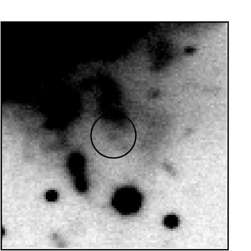
Figure 1.— A $21\arcsec.5\times 21\arcsec.5$ section of the combined LRIS $R$-band image centered on SN 2006gz taken with the 10-m Keck I telescope on 14 October 2007 (§2). North is up and east is to the left. The circle has a radius of 10 pixels, much larger than the uncertainty in the position of SN 2006gz (0.2 pixel).

Figure 1 shows a $21\arcsec.5\times 21\arcsec.5$ section of the LRIS image centered on SN 2006gz. The black circle has a radius of 10 pixels, which is much bigger than the astrometric transformation uncertainty (0.2 pixel), and is used for clarity in the figure. At the center of the circle, a faint stellar source is seen superimposed on some extended background emission; we regard this as a detection of SN 2006gz. Since the Subaru spectrum, although with poor S/N, shows broad features especially at $\sim$7200–7300 Å (§4.2), we conclude that other possibilities, such as an unrelated background object or an underlying H II region, are unlikely.

The photometric reduction was performed using the IRAF package DAOPHOT. The SN was detected by the automatic star detection routine DAOFIND, and then the photometry was performed via PSF fitting. We obtain the $R$ magnitude of the SN using the $R$ magnitude of field stars derived from the September Subaru image. For the $g$ magnitude, the Subaru $B$ and $V$ images for the field stars are used, with transformation equations from $B$ and $V$ to $g$ given by Fukugita et al. (1996). The photometry results in $m_{g}=25.5\pm 0.2$ and $m_{R}=25.5\pm 0.3$ mag.

In November the SN was not detected in the Subaru images. Because of the mediocre seeing, we did not obtain a meaningful $3\sigma$ limit: $m_{R}>23.3$ mag.

Table 3SN Ia Models

Name	$M_{\rm wd}$	$f_{ECE}$	$f_{\rm 56Ni}$	$f_{\rm IME}$	$M$(56Ni)	$E_{\rm k}$
SW7	1.39	0.18	0.43	0.32	0.6	1.40
LW7	1.39	0.00	0.72	0.21	1.0	1.41
SupCh2	2.00	0.21	0.50	0.22	1.0	1.60
SupCh3	3.00	0.14	0.33	0.46	1.0	1.50

3. SN Ia MODELS

To quantify the observational results, we have constructed four SN Ia models, based on the W7 model of Nomoto, Thielemann, & Yokoi (1984), which reproduces the basic observational features of normal SNe Ia (Branch et al. 1985). Our model contains the following five parameters (see also Howell et al. 2006; Jeffery et al. 2006): $M_{\rm wd}$ (progenitor WD mass), $\rho_{\rm wd}$ (WD central density, set to be $3\times 10^{9}$ g cm^-3 throughout this paper), $f_{\rm ECE}$ (mass fraction of electron capture Fe-peak elements, e.g., ⁵⁴Fe, ⁵⁶Fe, ⁵⁸Ni), $f_{\rm 56Ni}$ (mass fraction of ⁵⁶Ni), and $f_{\rm IME}$ (mass fraction of partially burned intermediate-mass elements). The kinetic energy of the ejecta ($E_{\rm K}$) is given as a function of these parameters, as this is the nuclear energy generation reduced by the binding energy of the WD. We use the binding energy formulae from Yoon & Langer (2005), whose models include rotating SupCh-WDs. We adopt the density distribution of the W7 model as a function of the velocity, and scale it in a self-similar way: $\rho(v)\propto M_{\rm wd}^{5/2}E_{\rm K}^{-3/2}$ and $v\propto M_{\rm wd}^{-1/2}E_{\rm K}^{1/2}$. The distribution of the elements is assumed to be concentric, and ordered as follows: ECE, ⁵⁶Ni, IME, then unburned C+O from the innermost region. Table 3 summarizes our models: SW7 (Simplified W7), LW7 (Luminous W7), SupCh2 and SupCh3 (Super-Chandrasekhar models), characterized by different $M_{\rm wd}$ (progenitor WD mass), $M_{\rm 56Ni}$ (mass of ⁵⁶Ni synthesized at the explosion), and $E_{\rm K}$ (kinetic energy of the expanding ejecta).

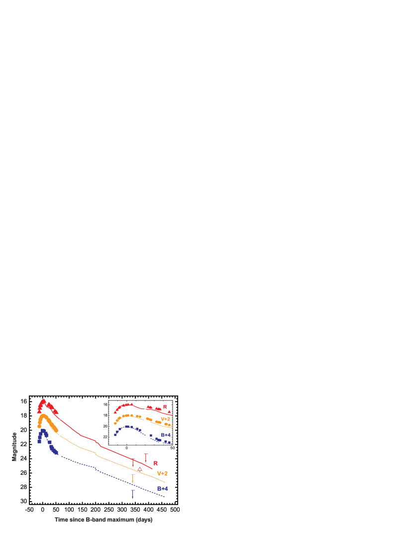
Figure 2.— $B$ (blue squares), $V$ (orange circles), and $R$ (red triangles) light curves of SN 2006gz as compared with those of SN Ia 2003du ($B$ is the blue dashed line; $V$ is the orange dotted line; $R$ is the red solid line). Each light curve of SN 2003du is arbitrarily shifted in magnitude so that they are normalized at the peak and have roughly the same peak magnitude as SN 2006gz ($\sim 16$ mag in all bands: Hicken et al. 2007), to more easily compare the light-curve shapes. SN 2003du represents a typical light-curve shape of SNe Ia (e.g., SN 2001el has an almost identical light-curve shape; Krisciunas, et al. 2003; Stritzinger & Sollerman 2007). For SN 2006gz, the early-phase data (filled symbols) are from Hicken et al. (2007), while the late-phase date (open symbols) are from our Subaru (upper limit on $+341$ d and $+390$ d) and Keck (open symbol, $+367$ d) observations. SN 2003du data are from Stanishev et al. (2007).

For these models, we compute bolometric light curves using a one-dimensional Monte-Carlo radiation transport code (Cappellaro et al. 1997; Maeda et al. 2003) with the phenomenological opacity description for optical photons ($\kappa_{\rm opt}$) given by Mazzali et al. (2001a), which crudely takes into account the largest contribution from the Fe-peak elements. This description has been tested for normal SNe Ia using W7-like models (Mazzali et al. 2001a). The transport of $\gamma$-rays from the ⁵⁶Ni/⁵⁶Co decays is treated in a gray approximation with $\kappa_{\gamma}=0.025$ cm^-2 g^-1, which is very accurate for any input models (Sutherland & Wheeler 1984; Maeda 2006). Positron transport is also solved in a simplified way. We assume a phenomenological opacity $\kappa_{e^{+}}=7$ cm² g^-1, a value that explains the slightly faster decline of late-time light curves of normal SNe Ia by increasing the fraction of escaping positrons (Cappellaro et al. 1997).

Synthetic nebular spectra are also computed at $t=t_{\rm peak}+341$ d (i.e., Subaru/FOCAS observation in September), where $t_{\rm peak}$ is obtained for each model by the light-curve calculations. Given the deposited luminosity, which is obtained in the same way as in the light-curve calculations, ionization-recombination equilibrium and rate equations are solved iteratively (Mazzali et al. 2001b; see also Maeda et al. 2006b). Since we have not tried to obtain detailed fits to the observed data, the light curve and spectrum synthesis calculations should be regarded only as indicative.

Table 4Synthetic Magnitudes

Days since $B$ maximum	Band	SW7	LW7	SupCh2	SupCh3	Observed
+341	$B$	24.5	23.9	23.7	23.2	$>$ 24.4 ($\sim$ 24.8)
	$V$	23.7	23.1	22.8	22.1	$>$ 24.2 ($\sim$ 25.0)
	$R$	24.8	24.3	23.9	23.0	$>$ 24.0 ($\sim$ 25.0)
	$m_{R}-m_{\rm Bol}$	0.4	0.4	0.4	0.5
+367	$R$	25.4	24.8	24.4	23.4	25.5
	$m_{R}-m_{\rm Bol}$	0.5	0.4	0.5	0.5

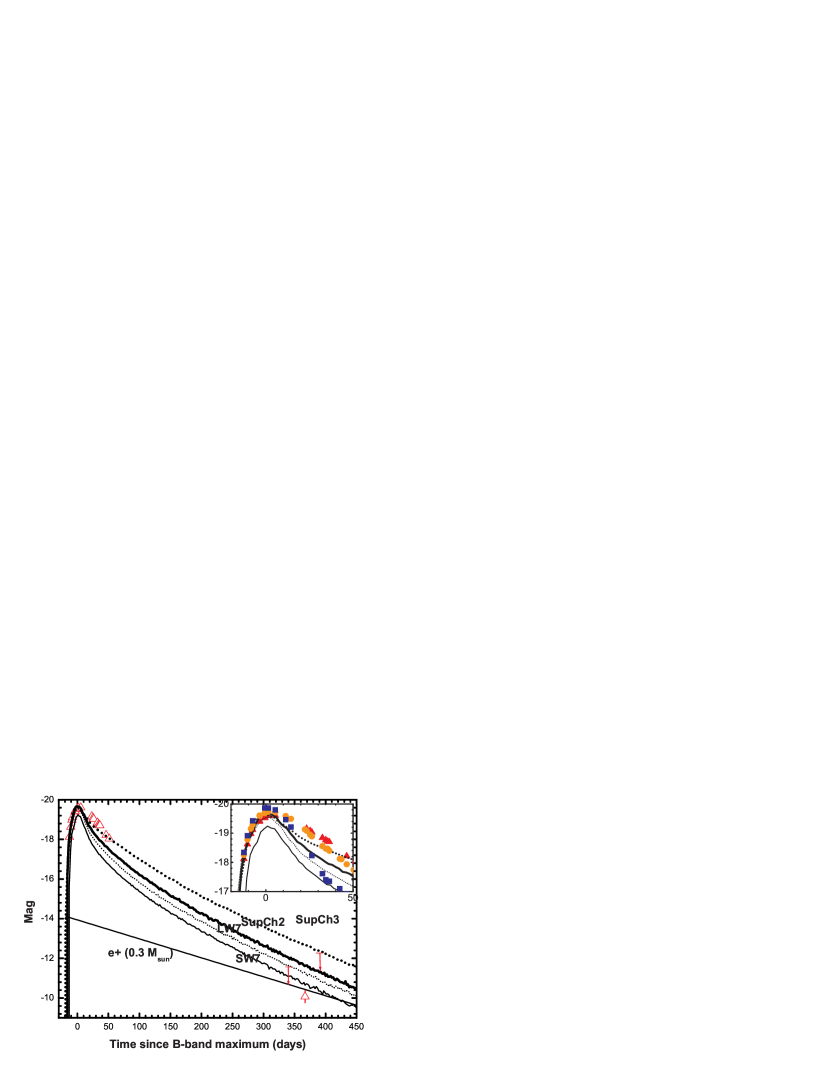
Figure 3.— Synthetic bolometric light curve for SN Ia models, as compared with the late-time $R$-band light curve of SN 2006gz (open triangles). Note that $m_{R}-m_{\rm Bol}=0.4$–0.5 mag for the models (§4.1 and Table 4). Models shown here are SW7 (thin solid; $t_{\rm peak}=17$ d), LW7 (thin dotted; $t_{\rm peak}=20$ d), SupCh2 (thick solid; $t_{\rm peak}=20$ d), and SupCh3 (thick dotted; $t_{\rm peak}=25$ d). Inserted figure is for the early-phase monochromatic light curves (Hicken et al. 2007), as compared with the same bolometric model light curves. We assume $\mu=34.95$ mag, $E(B-V)_{\rm host}=0.18$ mag, $E(B-V)_{\rm Gal}=0.063$ mag, and $R_{V}=3.1$ to convert the observed magnitudes to absolute magnitudes.

4. RESULTS

4.1. Light Curve: Rapid Fading

Figure 2 shows the results of our photometry as combined with the early-phase light curve of Hicken et al. (2007). The early post-maximum decline of SN 2006gz was slower in all bands than that of normal SNe Ia (Hicken et al. 2007), represented here by SN 2003du. However, this is not the case at the late phase: the detection of SN 2006gz in the $R$ band at $m_{R}=25.5\pm 0.3$ mag (Keck) and the $3\sigma$ upper limit in $B$ and $V$ (Subaru) show that eventually the visual luminosity of SN 2006gz declined more rapidly than that of other SNe Ia. Note that SN 2003du has a typical late-time light-curve shape, with a decline rate of 1.5–1.6 mag (100 d)^-1. There have been several SNe Ia whose decline is significantly slower (Lair et al. 2006), opposite to the behavior seen in SN 2006gz.

The September Subaru photometry ($+341$ d), $m_{R}>24.0$ mag, is consistent with the October Keck detection ($+367$ d) of SN 2006gz at $m_{R}=25.5\pm 0.3$ mag. The most likely magnitude at $t=t_{\rm peak}+341$ d is $m_{R}\approx 25.0$, $m_{V}\approx 25.0$, and $m_{B}\approx 24.8$ mag, assuming that the decline rate between these two epochs follows the ⁵⁶Ni heating model (see Table 4 for the model prediction).

Figure 3 shows the synthetic bolometric light curves of the four models as compared with the observed $R$-band light curve. Table 4 summarizes the synthetic multi-band magnitudes as derived from the model spectra. The late-time bolometric correction is $m_{R}-m_{Bol}=0.4$–0.5 mag for all the models presented here.

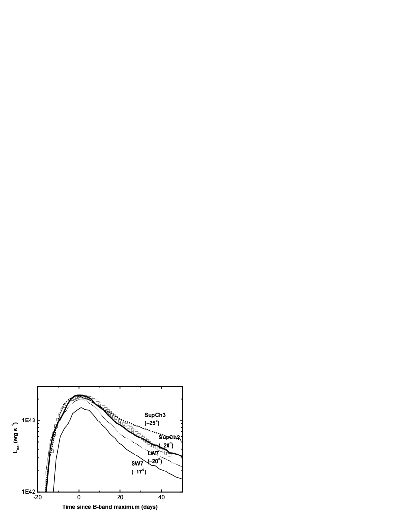
Figure 4.— Synthetic bolometric model light curves compared with the UBVRI bolometric light curve of SN 2006gz at early times (Hicken et al. 2007; see the footnote in the text). We assume $\mu=34.95$ mag, $E(B-V)_{\rm host}=0.18$ mag, $E(B-V)_{\rm Gal}=0.063$ mag, and $R_{V}=3.1$.

Figure 4 shows the synthetic bolometric light curves of the four models as compared with the observationally derived bolometric light curve of SN 2006gz [with $R_{V}=3.1$, $E(B-V)_{\rm host}=0.18$ mag, and $E(B-V)_{\rm Gal}=0.063$ mag]. The models with $M$(⁵⁶Ni) = 1 M_⊙ reproduce the peak magnitude fairly well. The behavior before the peak (except SW7) is very similar for different models despite different $t_{\rm peak}$. Thus, it seems difficult to constrain $t_{\rm peak}$ as accurately as $t_{\rm peak}=16.6\pm 0.6$ d mentioned by Hicken et al. (2007), and our models are consistent with the observed rising behavior. The different progenitor masses can be distinguished after the peak. A more massive progenitor results in a slower decline after the peak because of the larger diffusion time scale. From this point of view, Model SupCh2 with $M_{\rm wd}=2$ M_⊙ yields the light curve most consistent with the observations around the peak. In addition, the photospheric velocity and temperature at the peak luminosity, derived in the light-curve calculations, are similar in the SupCh2 and SW7 models. Within the uncertainties involved in the model calculations, these are consistent with the observed characteristics. Details of the early-phase characteristics will be presented elsewhere (K. Maeda, in preparation).

At late epochs, however, the models are more than 1 mag brighter than the observations, with the discrepancy reaching $\sim 2$ mag for SupCh2 and $\sim 3$ mag for SupCh3 in the $V$ band, where the models predict strong emission lines (see §4.2). Indeed, only model SW7 is marginally consistent with the late-time photometry, while the other three models having $M_{\rm 56Ni}=1$ M_⊙ are too bright compared to the observations.

The failure of the SupCh models stems from the larger binding energy of a WD and the higher density. The peak date ($t_{\rm peak}$) measured from the explosion date and the peak luminosity ($L_{\rm peak}$) are roughly estimated by the following relations (e.g., Arnett 1982):

$$t_{\rm peak} \approx 11\ \left(\frac{\kappa_{\rm opt}}{0.1\ {\rm cm}^{2}\ g^{-1}}\right)^{1/2}M_{{\rm wd},\odot}^{3/4}E_{{\rm K},51}^{-1/4}\ {\rm d},$$ (2)

$$L_{\rm peak} \approx 7.8\times 10^{43}\ M_{{\rm 56Ni},\odot}\exp\left(\frac{-t_{\rm peak}}{8.8~{}{\rm d}}\right)\ {\rm ergs}\ {\rm s}^{-1}\ .$$ (3)

Here the subscripts $\odot$ and $51$ mean that these values are expressed in units of M_⊙ and $10^{51}$ ergs, respectively. The optical depth to $\gamma$-rays from the ⁵⁶Co decay at late epochs ($t=t_{\rm tail}$) is expressed as follows (e.g., Clocchiatti & Wheeler 1997; Maeda et al. 2003):

$$\tau_{\gamma}\approx 1000\,M_{{\rm wd},\odot}^{2}E_{{\rm K},51}^{-1}\left(\frac{t_{\rm tail}}{{\rm d}}\right)^{-2}\ .$$ (4)

The luminosity at $t_{\rm tail}$ ($L_{\rm tail}$) is then estimated as

$$L_{\rm tail} \approx 1.3\times 10^{43}\,{\rm ergs}\ {\rm s}^{-1}M_{{\rm 56Ni},\odot}$$ (5)

$$\times(\tau_{\gamma}+0.035f_{e+})\exp\left(\frac{-t_{\rm tail}}{113.5~{}{\rm d}}\right)\ ,$$

where the factor 0.035 accounts for the positron contribution to the heating, with $f_{e+}$ being the fraction of positrons trapped within the ejecta ($f_{e+}\approx 1$ in usual situations). Using these expressions and values listed in Table 3, the expected bolometric magnitude difference between the peak and the tail ($t_{\rm tail}=t_{\rm peak}+341$ d) can be derived: $\Delta m_{\rm Bol}\approx 7.1$ mag for SW7 and LW7, and $6.5$ for SupCh2. This comes from the larger $t_{\rm peak}$ and the larger $\tau_{\gamma}$ in the SupCh2 model, as a result of the larger mass and binding energy of a WD (i.e., larger ratios of $M_{\rm wd}^{2}/E_{\rm K}$ and $M_{\rm wd}^{3}/E_{\rm K}$, in which $E_{\rm K}$ is reduced by the binding energy). This behavior, smaller $\Delta m_{\rm Bol}$ in the SupCh models, is independent of the uncertainty in distance and reddening.

Other model-independent constraints on $M_{\rm 56Ni}$ can be obtained considering the positron channel. Omitting the $\tau_{\gamma}$ term from eq. (5), we obtain an upper limit on $M_{\rm 56Ni}$ from the requirement that this positron luminosity should be below the observed luminosity (Fig. 3):

$$M_{\rm 56Ni}\mathrel{\hbox to0.0pt{\lower 4.0pt\hbox{\hskip 1.0pt$\sim$}\hss}\raise 1.0pt\hbox{$<$}}0.3{\rm M}_{\odot}f_{e+}^{-1}\ .$$ (6)

Here we adopted $m_{R}-m_{\rm Bol}=0.5$ mag, a typical value in the model spectrum synthesis calculations.

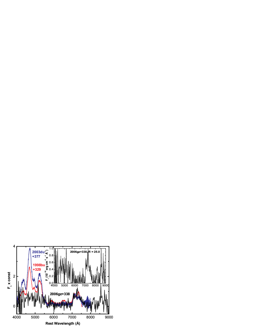
Figure 5.— Late-time Subaru spectrum of SN 2006gz at $t=t_{\rm p}+341$ d (black line) as compared with those of SNe Ia 2003du ($t_{\rm p}+377$ d, blue line; Stanishev et al. 2007) and 1998bu ($t_{\rm p}+329$ d, green line; Cappellaro et al. 2001). In this comparison, the flux is normalized at $\sim$7000–7500 Å. The insert is the Subaru spectrum, with the flux (in units of 10^-18 erg cm^-2 Å^-1) renormalized to give $m_{R}=25.0$ mag (see §4.1 and Table 4). Wavelengths are in the rest flame (using $z=0.02363$ for SN 2006gz). The spectrum is smoothed with a binning width of 22.4 Å. The data for SNe 2003du and 1998bu are from the SUSPECT database (see the footnote in the text).

4.2. Spectrum: Missing [Fe II] and [Fe III] in the Blue

Figure 5 shows the late-time spectrum of SN 2006gz and the comparison with spectra of other SNe Ia. In SN 2006gz, the emissions at $\sim$4700 Å ([Fe II] $\lambda\lambda$4814, 4890, 4905; [Fe III] $\lambda\lambda$4858, 4701) and at $\sim$5200 Å ([Fe II] $\lambda\lambda$5159, 5262) are extremely weak or undetected. The only confirmed detection is at $\sim$7200–7300 Å, which is interpreted as the blend of [Fe II] $\lambda\lambda$7151, 7171, 7388, 7452 in SNe Ia. This feature may also be [Ca II] $\lambda\lambda$7291, 7324 as commonly seen in core-collapse SNe (see §5).

Indeed, in the SUSPECT database we found only one example of a SN Ia that probably shows a feature at $\sim$7200–7300 Å as strong as the [Fe II] and [Fe III] in the blue. This is the underluminous SN 1991bg (Filippenko et al. 1992), with $M_{\rm 56Ni}\approx 0.1$ M_⊙(Mazzali et al. 1997). Thus, SN 2006gz does not appear to follow the behavior of normal SNe Ia, both in the light-curve shape (Hicken et al. 2007) and in the late-time spectral features.

Figure 6 shows the synthetic spectra computed for the four models. There is a tendency for more-massive models to show a weaker flux in the [Fe II]–[Fe III] emission at $\mathrel{\hbox to0.0pt{\lower 4.0pt\hbox{\hskip 1.0pt$\sim$}\hss}\raise 1.0pt\hbox{$<$}}$5200 Å relative to the [Fe II] line near 7200 Å. An important quantity to characterize the relative line strengths is the ratio of density to heating rate per mass: generally, as this ratio increases, ionization (competing with recombination) and temperature (competing with the line emission) decrease, resulting in the stronger 7200 Å feature (corresponding to the lower ionization state and temperature). More-massive models have the larger ratio (e.g., in SupCh2 the density is a factor of 2, but the heating rate only a factor of 1.3, larger than in model SW7), but it is not sufficiently large to reproduce the observed, extremely large ratio of the red to the blue emission.

Figure 6.— Synthetic late-time spectra of the SN Ia models. The model flux is converted to the observed flux using the distance modulus and reddening shown in the caption of Figure 3. For clarity, an arbitrary constant is added to the flux for each model ($+5,+10$, and $+15\times 10^{-18}$ erg cm^-2 s^-1 Å^-1 for LW7, SupCh2, and SupCh3, respectively).

5. DISCUSSION AND CONCLUSIONS

We have presented late-time photometry and spectroscopy of SN 2006gz obtained with the Subaru and Keck I telescopes. These are the first late-time observational data for an SN Ia that was claimed to be overluminous at early phases. Such SNe have been suggested to be the explosions of SupCh-WD progenitors.

The spectrum is characterized by the weakness of the [Fe II] and [Fe III] lines in the blue ($\mathrel{\hbox to0.0pt{\lower 4.0pt\hbox{\hskip 1.0pt$\sim$}\hss}\raise 1.0pt\hbox{$<$}}5200$ Å) relative to emission lines in the red (either [Fe II] or [Ca II] at $\sim 7200$ Å). This does not fit into the sequence of the late-time spectral behavior of normal SNe Ia, confirming that SN 2006gz belongs to a different subclass of objects than normal SNe Ia. Coupled with this is the problem of the observed faintness of SN 2006gz, especially in the $V$ band.

The SupCh2 model (with a 2 M_⊙ WD progenitor synthesizing 1 M_⊙ of ⁵⁶Ni) is in good agreement with the early-phase bolometric light curve (§4.1; but see §5.1), although it predicts a higher late-time luminosity than the Ch-SN Ia models because of the larger $M_{\rm 56Ni}$ and $\gamma$-ray deposition rate. The luminosity of Sup-Ch models exceeds that observed by more than 2 mag in the $V$ band. Furthermore, one derives $M_{\rm 56Ni}\mathrel{\hbox to0.0pt{\lower 4.0pt\hbox{\hskip 1.0pt$\sim$}\hss}\raise 1.0pt\hbox{$<$}}0.3$ M_⊙, under the usual assumptions that the bulk of the deposited radioactive luminosity emerges at visual wavelengths, and that positrons are almost fully trapped within the ejecta. In what follows, we list possible solutions for this inconsistency.

5.1. Reconsidering the Super Chandrasekhar Model?

We should first mention that the peak luminosity of SN 2006gz derived by Hicken et al. (2007) involves large uncertainty, as the host-galaxy extinction is not well constrained. If the host extinction is negligible, the peak luminosity of SN 2006gz is close to that of normal SNe Ia ($M_{V}=-19.19$ mag). In this case, SN 2006gz might be a less energetic explosion of a Ch-WD, possibly because of insufficient burning of the C-O layer to intermediate-mass elements, to be consistent with the observed slow light-curve evolution at early times. It is not clear if the early-phase spectroscopic features can be explained by this model: the early-phase spectra (Hicken et al. 2007) indicate that the photospheric temperature is high (e.g., the weak Si II 5972) and the velocity is normal ($v_{\rm Si~{}II}\approx 11,000$–12,000 km s^-1 at $B$-band maximum). Thus, the most straightforward interpretation is that the peak luminosity is also high. Although the Ch-WD model is an interesting possibility and deserves further investigation, it should not affect most of our conclusions about the peculiar late-time behavior, as our arguments are based mainly on the magnitude difference between the peak and the tail. In what follows, we assume the host extinction adopted by Hicken et al. (2007), but the above caveat should be kept in mind.

From the late-time data, we find that $m_{V}$ is $\sim 1.3$ and $\sim 2.2$ mag larger (that is, fainter) than expected from the SW7 ($M_{\rm 56Ni}=0.6$ M_⊙) and SupCh2 ($M_{\rm 56Ni}=1.0$ M_⊙) models, respectively. This would imply that 0.1–0.2 M_⊙ of ⁵⁶Ni powers the late-time emission, smaller than the value expected from the light-curve peak ($M_{\rm 56Ni}\approx 1$ M_⊙) by a factor of $\mathrel{\hbox to0.0pt{\lower 4.0pt\hbox{\hskip 1.0pt$\sim$}\hss}\raise 1.0pt\hbox{$>$}}5$. Such a large discrepancy cannot be attributed solely to the effect of viewing angle, even if SN 2006gz was a result of an extremely off-axis explosion (see, e.g., Sim et al. 2007 for the effect of viewing angle; see also Maeda, Mazzali, & Nomoto 2006a).

Alternatively, one may hypothesize that the energy source at early times was not ⁵⁶Ni/Co/Fe decay. Strong circumstellar interaction as seen in a peculiar class of SNe Ia (i.e., SNe Ia/IIa 2002ic-like events: Hamuy et al. 2003; Deng et al. 2004; Wang et al. 2004) is not favored, because of the lack of evidence for interaction in the early-phase spectra. Moreover, the SupCh models yield a reasonable fit to the early-time UBVRI bolometric light curve without the fine tuning of parameters. The early-phase spectroscopic features also seem to be consistent with SupCh models (§4.2; K. Maeda, in preparation). Thus, ⁵⁶Ni/Co energy input is the most likely mechanism to power the early-phase emission.

5.2. Positron Escape, Infrared Catastrophe, or Dust Formation?

If the early-phase emission is powered by $\sim 1$ M_⊙ of ⁵⁶Ni, then one is left with the possibility that some mechanism, which is not at work in normal SNe Ia, must be affecting the late-time emission and the thermal conditions within the ejecta of SN 2006gz.

One possibility is the escape of positrons produced by the ⁵⁶Co decay out of the SN ejecta. The issue has been comprehensively explored by Milne, The, & Leising (2001). They showed that a fraction of the positrons can escape for a radially combed and/or weak magnetic field, leading to the changing light curve at late times. However, at $t\approx 400$ d, this effect can account for at most $\sim 0.5$ mag, which is not large enough to completely remedy the present problem.

Another possibility is the thermal catastrophe within the ⁵⁶Ni-rich region, which shifts the bulk of the emission from optical to infrared wavelengths (Axelrod 1988). This so-called “infrared catastrophe” (IRC) is expected to take place after the temperature drops below a few 1000 K, depending on the electron density. Observationally, the IRC has not been clearly detected in any SNe Ia. The IRC does not take place at $t\approx 1$ yr in any of our models: the heating rate per unit volume in the Fe-rich emission region is only a factor of $\sim 1.5$ smaller in SupCh2 than in SW7, and thus the thermal conditions are similar in the two models.

Finally, it may be possible that the visual light from the ⁵⁶Ni-rich region is converted to near-IR/mid-IR wavelengths by dust formed in the C+O-rich region. Before maximum light, SN 2006gz showed the strongest C lines of any SN Ia ever observed, with little evolution in the absorption velocity. This indicates that a dense C+O-rich shell or clumps are present in SN 2006gz, at least in the outermost region. The presence of carbon may be a key to the understanding of the peculiar behavior at late phases, since carbon has a relatively high condensation temperature.

The W7 model has $n\approx 10^{7}$ cm^-3 at the inner edge of the C+O-rich region at 100 d after the explosion. The corresponding density in the SupCh models is a few times higher. Recently, Nozawa et al. (2008) theoretically investigated dust formation in SNe Ib. They found a large amount of carbon grain formation in the C-enhanced outer He region, with a density comparable to that in the SN Ia models, in their model at $t\mathrel{\hbox to0.0pt{\lower 4.0pt\hbox{\hskip 1.0pt$\sim$}\hss}\raise 1.0pt\hbox{$>$}}50$ d. Thus, carbon grain formation in SNe Ia may also be possible if carbon is abundant in the outermost region. For normal SNe Ia, accelerated fading like that of SN 2006gz has never been reported. This may be consistent with the estimate that the upper limit of the carbon mass fraction is as low as 0.01 (e.g., Tanaka et al. 2008). Details of the dust formation process, addressing the difference between SN Ib and SN Ia models (heating rate by ⁵⁶Ni, different oxygen mass fraction, etc.), should be investigated, as well as details of expected observational signatures during the dust formation. In this interpretation, a part of the outer Ca-rich region might be mixed with the C+O-rich region. It may partly explain the relative strength of the feature at $\sim 7300$ Å relative to the [Fe II] and [Fe III] in the blue, since [Ca II] arising from the Ca-rich region could be less diluted than the Fe emission, contributing to the 7300 Å feature.

5.3. Future Observations

The possible interpretations we listed above are only speculative, but they predict distinct observational signatures, to be tested in future overluminous SNe Ia. First, late-time spectroscopy of other potentially overluminous SNe Ia would be extremely useful to see whether SN 2006gz is special even among these peculiar SNe Ia. If some of them show the SN 2006gz-like peculiarities at late phases, the optical light curves spanning from early to late times should provide a probe: (a) the IRC and dust scenarios predict a sudden decrease in the visual luminosity, (b) the positron-escape scenario would manifest itself with a relatively gentle decrease of the luminosity, and (c) other heating scenarios would not necessarily follow the quasi-exponential decline.

Near-IR light curves could directly show the effects of the IRC and dust distinctly from other scenarios: we expect that a rapid increase in the near-IR brightness should occur simultaneously with a rapid decrease in the visual brightness, while other scenarios do not necessarily predict this behavior.

A temporal sequence of optical spectra would also be highly useful. In the dust formation scenario, we may see a transient red continuum and emission-line shifts at intermediate phases, as was seen in the peculiar SN Ib 2006jc (Smith, Foley, & Filippenko 2008).

Finally, the IRC and dust scenarios could be unambiguously distinguished with near-IR through mid-IR spectra. Blackbody radiation from the dust particles should be seen in the dust scenario, while line emission is the dominant cooling process in the IRC scenario.

References

- (1) Arnett, W. D., 1982, ApJ, 253, 785
- (2) Axelrod, T.S. 1988, in IAU Colloquium 108, Atmospheric Diagnostics in Stellar Evolution: Chemical Peculiarity, Mass Loss, and Explosion, (Lecture Notes in Physics, 305), ed. K. Nomoto (Berlin: Springer Verlag), 375
- (3) Branch, D., Fisher, A., & Nugent, P. 1993, AJ, 106, 2383
- (4) Branch, D., Doggett, J. B., Nomoto, K., & Thielemann, F.-K. 1985, ApJ, 294, 619
- (5) Cappellaro, E., Mazzali, P. A., Benetti, S., Danziger, I. J., Turatto, M., Della Valle, M., & Patat, F. 1997, A&A, 328, 203
- (6) Cappellaro, E., et al. 2001, ApJ, 549, L215
- (7) Clocchiatti, A., & Wheeler, J. C. 1997, ApJ, 491, 375
- (8) Deng, J., et al. 2004, ApJ, 605, L37
- (9) Filippenko, A. V. 1982, PASP, 94, 715
- (10) Filippenko, A. V. 2005, in White Dwarfs: Cosmological and Galactic Probes, ed. E. M. Sion, S. Vennes, & H. L. Shipman (Dordrecht: Springer), 97
- (11) Filippenko, A. V., Li, W., Treffers, R. R., & Modjaz, M. 2001, in Small-Telescope Astronomy on Global Scales, ed. W.-P. Chen, C. Lemme, & B. Paczyński (ASP Conf. Ser. 246; San Francisco: ASP), 121
- (12) Filippenko, A. V., et al. 1992, AJ, 104, 1543
- (13) Fukugita, M., Ichikawa, T., Gunn, J. E., Doi, M., Shimasaku, K., & Schneider, D. P. 1996, AJ, 111, 1748
- (14) Hamuy, M., et al. 2003, Nature, 424, 651
- (15) Hicken, M., et al. 2007, ApJ, 669, L17
- (16) Hillebrandt, W., & Niemeyer, J. C. 2000, ARAA, 38, 191
- (17) Hillebrandt, W., Sim, S. A., & Röpke, F. 2007, A&A, 465, 17
- (18) Howell, D. A., et al. 2006, Nature, 443, 308
- (19) Jeffery, D. J., Branch, D., & Baron, E. 2006, preprint (astro-ph/0609804)
- (20) Kashikawa, N., et al. 2002, PASJ, 54, 819
- (21) Khoklov, A., Müller, E., & Höflich, P. 1993, A&A, 270, 223
- (22) Krisciunas, K., et al. 2003, AJ, 125, 166
- (23) Lair, J. C., Leising, M.D., Milne, P.A., & Williams, G.G. 2006, AJ, 132, 2024
- (24) Landolt, A. U. 1992, AJ, 104, 340
- (25) Li, W., Filippenko, A. V., Treffers, R. R., Riess, A. G., Hu, J., & Qiu, Y. 2001, ApJ, 546, 734
- (26) Livio, M. 2000, in Type Ia Supernovae: Theory and Cosmology, ed. J. C. Niemeyer & J. W. Truran (Cambridge: Cambridge University Press), 33
- (27) Maeda, K. 2006, ApJ, 644, 385
- (28) Maeda, K., Mazzali, P. A., Deng, J., Nomoto, K., Yoshii, Y., Tomita, H., & Kobayashi, Y. 2003, ApJ, 593, 931
- (29) Maeda, K., Mazzali, P. A., & Nomoto, K. 2006a, ApJ, 645, 1331
- (30) Maeda, K., Nomoto, K., Mazzali, P. A., & Deng, J. 2006b, ApJ, 640, 854
- (31) Massey, P., & Gronwall, C. 1990, ApJ, 358, 344
- (32) Mazzali, P. A., et al. 1997, MNRAS, 284, 151
- (33) Mazzali, P. A., Nomoto, K., Cappellaro, E., Nakamura, T., Umeda, H., & Iwamoto, K. 2001a, ApJ, 547, 988
- (34) Mazzali, P. A., Nomoto, K., Patat, F., & Maeda, K. 2001b, ApJ, 559, 1047
- (35) Milne, P. A., The, L.-S., & Leising, M. D. 2001, ApJ, 559, 1019
- (36) Nomoto, K., Thielemann, F.-K., & Yokoi, K. 1984, ApJ, 286, 644
- (37) Nomoto, K., Iwamoto, K., & Kishimoto, N. 1997, Science, 276, 1378
- (38) Nomoto, K., Uenishi, T., Kobayashi, C., Umeda, H., Ohkubo, T., Hachisu, I., & Kato, M. 2003, in From Twilight to Highlight: The Physics of Supernovae, ed. W. Hillebrandt & B. Leibundgut (Berlin: Springer), 115 (astro-ph/0308138)
- (39) Nozawa, T., et al. 2008, ApJ, in press (astro-ph/0801.2015)
- (40) Oke, J. B., et al. 1995, PASP, 107, 375
- (41) Perlmutter, S., et al. 1999, ApJ, 517, 565
- (42) Phillips, M. M. 1993, ApJ, 413, L105
- (43) Phillips, M. M., Lira, P., Suntzeff, N. B., Schommer, R. A., Hamuy, M., & Jose, M. 1999, AJ, 118, 1766
- (44) Riess, A. G., et al. 1998, AJ, 116, 1009
- (45) Sim, S. A., Sauer, D. N., Röpke, F. K., & Hillebrandt, W. 2007, MNRAS, 378, 2
- (46) Smith, N., Foley, R. J., & Filippenko, A. V. 2008, ApJ, 680, 568
- (47) Sollerman, J., et al. 2004, A&A, 428, 555
- (48) Stanishev, V., et al. 2007, A&A, 469, 645
- (49) Stritzinger, M., & Sollerman, J. 2007, A&A, 470, L1
- (50) Sutherland, P. G., & Wheeler, J. C. 1984, ApJ, 280, 282
- (51) Tanaka, M., et al. 2008, ApJ, 677, 448
- (52) Uenishi, T., Nomoto, K., & Hachisu, I. 2003, ApJ, 595, 1094
- (53) Wang, L., Baade, D., Höflich, P., Wheeler, J. C., Kawabata, K., & Nomoto, K. 2004, ApJ, 604, L53
- (54) Yoon, S.-C., & Langer, N. 2004, A&A, 419, 623
- (55) Yoon, S.-C., & Langer, N. 2005, A&A, 435, 967
- (56) Yuan, F., et al. 2007, ATEL 1212