PYRAMIR: Calibration and operation of a pyramid near-infrared wavefront sensor

Abstract

The concept of pyramid wavefront sensors (PWFS) has been around about a decade by now. However there is still a great lack of characterizing measurements that allow the best operation of such a system under real life conditions at an astronomical telescope.
In this article we, therefore, investigate the behavior and robustness of the pyramid infrared wavefront sensor PYRAMIR mounted at the 3.5 m telescope at the Calar Alto Observatory under the influence of different error sources both intrinsic to the sensor, and arising in the preceding optical system. The intrinsic errors include diffraction effects on the pyramid edges and detector read out noise.
The external imperfections consist of a Gaussian profile in the intensity distribution in the pupil plane during calibration, the effect of an optically resolved reference source, and noncommon-path aberrations. We investigated the effect of three differently sized reference sources on the calibration of the PWFS. For the noncommon-path aberrations the quality of the response of the system is quantified in terms of modal cross talk and aliasing. We investigate the special behavior of the system regarding tip-tilt control.
From our measurements we derive the method to optimize the calibration procedure and the setup of a PWFS adaptive optics (AO) system. We also calculate the total wavefront error arising from aliasing, modal cross talk, measurement error, and fitting error in order to optimize the number of calibrated modes for on-sky operations. These measurements result in a prediction of on-sky performance for various conditions.

D. Peter, M. Feldt, B. Dorner, T. Henning, S. Hippler, J. Aceituno
      1, Max-Planck-Institut für Astronomie, Königstuhl 17, 69117 Heidelberg, Germany
      2, Centro Astronómico Hispanio Alemán, C/ Jesús Durbán Remón, 2-2, 04004 Almeria, Spain

1 Introduction

Within the context of AO systems pyramid wavefront sensors (PWFS) are a relatively novel concept. The special interest in this concept arises from the prediction of a gain in sensitivity – and thus in limiting magnitude – for a nonmodulated PWFS over a Shack-Hartmann sensor (SHS) [Ragazzoni & Farinato (1999)] in closed-loop conditions for a well-corrected point source. The definition of this gain is that in order to achieve the same correction quality the PWFS needs less signal than the SHS. This gain in sensitivity results basically from the fact that the accuracy of the measurement and the resulting reconstruction error $\sigma^{2}_{SH}$ of the SHS depends on $\lambda\over{d_{sub}}$ with $\lambda$ = sensing wavelength, $d_{sub}$ = subaperture size typically chosen on the order of the Fried-parameter $r_{0}$ for typical site seeing at science wave-length. In the case of the PWFS the measurement error $\sigma^{2}_{P}$ depends on $\lambda\over{D}$ with $D$ being the telescope diameter ($D>>r_{0}$). From these formulas the difference in stellar magnitudes that are needed to achieve the same Strehl ratio for the exemplary case of tip-tilt only can be derived for both sensors as $\Delta m=-2.5log\left({\sigma_{P}^{2}\over{\sigma_{SH}^{2}}}\right)\approx-2.5log\left({r_{0}^{2}\over{D^{2}}}\right)$. Simulations show , for instance, [Ragazzoni & Farinato (1999)] that the gain in sensitivity for a 4 m class telescope and a seeing of $0.5^{\prime\prime}$ ($r_{0}=20$ cm) is predicted to be 2 magnitudes.

1.1 The Pyramid Principle

Wavefront sensing based on the pyramid principle has its origin in the Foucault knife-edge test. The historical development of the PWFS is described in [Campbell & Greenaway(2006)].

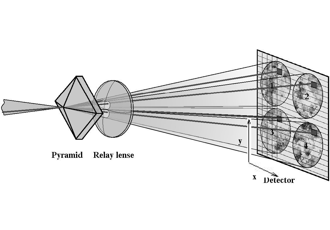
Figure 1: (Courtesy of S. Egner) The pyramid principle. An example of corresponding pixels is marked. The gradient in this position of the pupil is calculated from the intensity differences in between these pixels.

The optical setup of a pyramid sensor is shown in Figure 1. The transmissive, four-sided pyramid prism is placed in the focal plane. The focus is placed on the tip of the pyramid. After the pyramid, a relay lens images the pupils onto the detector.
The signal a four-sided AO PWFS system uses are the intensities inside four pupil images. The illumination of these images depends on the aberrations of the wavefront. The signal $S$ one extracts is the difference in intensities $I_{1,2,3,4}$ between corresponding pixels in the four pupils ,i.e., the pixels at the same optical position in the pupils as shown in Fig.1:

$$S_{x}(x,y)={{I_{1}(x,y)+I_{3}(x,y)-[I_{2}(x,y)+I_{4}(x,y)]}\over{I_{1}(x,y)+I_{2}(x,y)+I_{3}(x,y)+I_{4}(x,y)}}$$ (1)

$$S_{y}(x,y)={{I_{1}(x,y)+I_{2}(x,y)-[I_{3}(x,y)+I_{4}(x,y)]}\over{I_{1}(x,y)+I_{2}(x,y)+I_{3}(x,y)+I_{4}(x,y)}}$$ (2)

for the x- and y-direction, respectively. These signals $S$ are what we will refer to as gradients, even if they might not exactly represent wavefront gradients. In the limit of small perturbations and a telescope with infinite aperture the frequency spectrum of the signal $S_{x}$ of our sensor is given by

$$\widetilde{S_{x}}=i{\rm sgn}(u)\widetilde{\phi}(u,v).$$ (3)

Here $\widetilde{()}$ means Fourier transform, $\phi(u,v)$ the phase of the electromagnetic wave with $u$ and $v$ the coordinates in Fourier space, and sgn the sign-function (see [Costa(2003)]). Thus the sensor is working as a phase sensor in this regime.
The principle of the PWFS implies some limitations that either do not occur in other sensor types, or have a much more ”dramatic” impact on PWFSs than on other sensor types. In this class fall the structure of the pyramid edges that cause both diffraction and scattering, the read out noise of the system, the goodness of centering the beam on the pyramid tip, noncommon-path aberrations, and the homogeneity of the pupil illumination, the latter being important especially during calibration. It is these limitations, that may ultimately influence the choice of this or another sensor type, that will be examined in the course of this article.
The structure in the remaining part of the article is as follows: In the next section, the PYRAMIR system is described in detail. The optical path and the possible detector read out modes are explained. Section 3 accounts for the calibration procedure of the system. The peculiarities of tip-tilt calibration and flattening the wavefront are presented. Section 4 shows fundamental limitations to the performance of a pyramid system. “Fundamental” in this case is not meant to be based on natural laws and constants, but on always-present aberrations and nonideal conditions. Thus, the fundamental limitations discussed here can be eased by careful alignment and set up of the system, but they can never entirely be removed. In this context, we explore the effect of static aberrations, different calibration light sources, and diffraction and scattering on the pyramid edges to the response of the system. In the next section the implications of the modal cross talk of the system aliasing and measurement error to the number of modes to be calibrated, and the residual wavefront error are calculated. We end the section with a prediction of the on-sky performance under different seeing conditions. The last section concludes the results of our measurements and the implications for any pyramid wavefront sensor.
On-sky results will be presented in a following paper [Peter et al.(2008)].

2 The PYRAMIR System

PYRAMIR is a PWFS working in the effective wavelength regime between 1.26 and 2.4 $\mu$m (J,H,K-Bands). It is integrated into the ALFA-system at the 3.5m telescope of the Calar Alto observatory.

Table 1: Properties of the PYRAMIR system

length	1.1m
diameter	0.206 m
weight	35 kg
Detector temperature	78 K
Temp. stability	$\geq$ 24h
mount	xyz-stage moved by stepper motors
step size	10$\mu$m
beam splitter	P90O10, P20O80, K/J

The properties of the system are shown in Table 1. The beam splitter can be exchanged manually. Here, the choice is between 90% light on PYRAMIR and 10% on the science camera (P90O10), 20% on PYRAMIR and 80% on the science camera (P20O80), or K-band on PYRAMIR and J-band on the science camera.

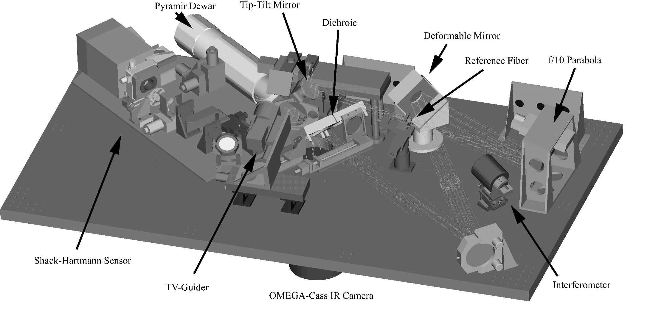
Figure 2: Setup of the adaptive optics bench ALFA.

The optical path in the ALFA-system is shown in Fig.2. Coming from the telescope the beam passes the mirror for tip-tilt (TT) correction. The position of the telescope focus is downstream from the TT-mirror. At the telescope’s F/10 focal plane a calibration fiber can be introduced into the beam. An off-axis parabola (F/10) is used to produce a collimated beam for the illumination of the deformable mirror (DM, Xinetics 97 actuator). The light is again focused by another off-axis parabola (F/25) and then divided into the science and WFS-paths by the beam splitter of choice (see table 1).

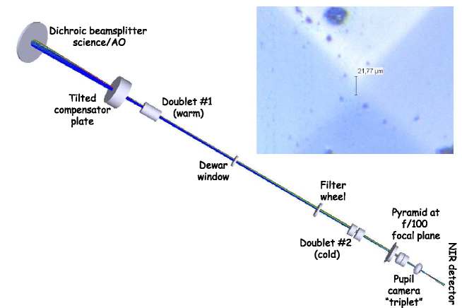
Figure 3: PYRAMIR arm of the system.

In the PYRAMIR arm (Fig.3) first a compensator plate compensates the static and chromatic aberrations introduced by the beam-splitter in the noncollimated beam. Then the light enters the PYRAMIR system. A warm lens doublet together with a corresponding cold doublet inside the dewar transforms the f/25 into a f/100 beam focused onto the tip of the pyramid. The tip size of the pyramid is about 20 $\mu$m and the diffraction-limited point-spread function (PSF) in the K-band has a full width at half-maximum (FWHM) of $\approx$ 220 $\mu$m. The wavelength of correction can be chosen according to Table 2. Additionally a spatial filter is introduced in front of the pyramid to reduce aliasing effects, to minimize the sky background, and to enable sensing on reasonably wide binaries.

Table 2: Properties of the PYRAMIR camera

Number of subapertures	224
Detector	Hawaii I
Pixel size	18 $\mu$m
maximum frame rate	$\approx$ 330 Hz
frame size	4 $\times$ 20x20 pixel
field stops	1”, 2”
Filters	J, H, K, H+K
system gain	3.8 $e^{-}$/ADU
RON	20 $e^{-}$

The possible sizes of the field stop are also given in Table 2. The final image is formed by a lens-triplet onto the IR detector. The pupil diameter on the detector is about 320 $\mu$m. In order to place the detector in the pupil plane while keeping the focus on the tip of the pyramid, one can move the detector in the direction of the optical axis by about 2 mm. The details of the PYRAMIR detector are shown in table 2.

2.1 Read out Modes

The detector, a Rockwell Hawaii I device, can be read out with three different read out modes. Only two of these three modes are used during operation: the line interlaced read (lir) and the multiple sampling read (msr).

Table 3: Read out modes of the PYRAMIR system

name	Pattern	Integration Time	Maximum speed	Comments
rrr	reset-read-read	50 %	165 Hz	lab use only
lir	read-reset-read	100 %	165 Hz	–
msr	reset-read-read-read-…	100 %	330 Hz	loose frame

For specifications see Table 3.

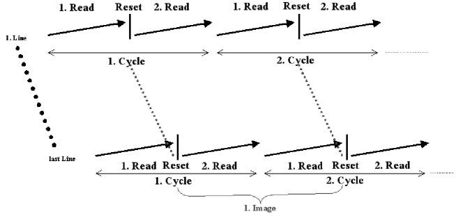
Figure 4: Read out pattern for the lir mode. Each line is read, reset, and read again before the next line is started. The image is built by the difference between the first frame of the second read and the second frame of the first read.

The lir mode is a line-oriented mode with the read out pattern read-reset-read, that is performed line by line. In this mode one line is read then reset and read again. This procedure is then continued for the next line until the whole array is read. The integration time for the image is the time between the second read of one pattern and the first read of the next (see Fig.4). With this scheme, almost 100$\%$ of the cycle time can be used as integration time (minus the reset time).
The msr mode is frame-oriented, i.e., one resets the whole array, reads the whole array, reads again the whole array etc. The pattern also differs from the lir mode.

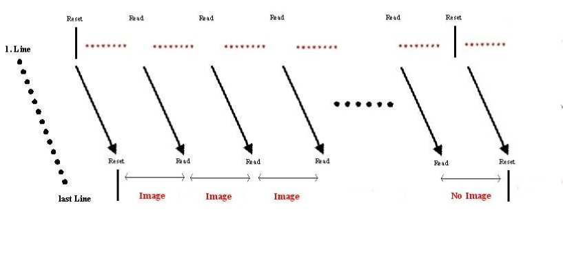
Figure 5: Read out pattern for the msr mode. The first image is constructed as the difference between the first read and a reset frame. The following images are built by the difference between two neighboring reads. The total signal on the detector is accumulated. The image between the second reset and the last read is lost.

First the detector is reset and then one only reads out: reset-read-read-read-… as shown in Fig.5. The signal is accumulated and the images used are difference images between two neighboring read out frames. Thus the images $I_{i}$ are produced by resets $Res_{i}$ and reads $R_{i}$ as follows:

$$I_{1}=R_{1}-Res_{1},\,I_{2}=R_{2}-R_{1},\,I_{3}=R_{3}-R_{2},/,I_{4}=R_{4}-R_{3}...$$ (4)

In order not to saturate the detector while accumulating signal one has to specify a maximum number of frames. For a star of fifth magnitude at 100 Hz this maximum number is of the order of 100 frames ($\approx$ 1s integration). The pattern runs up to the maximum frame and then starts again. With this pattern one will loose the frame at the end of every ramp : $Res_{2}-R_{n}$. Two features are obvious here: first one can read out twice as fast as with the lir mode because each image needs one read only, secondly already as mentioned one looses the image between the last read and the reset of the following pattern. This means one performs one step with half the applied loop frequency.

3 Calibration

3.1 Tip-Tilt Calibration

Because the TT-mirror is located upstream of the calibration light source, the TT-modes and the high-order (HO) modes are calibrated differently. For TT-calibration a ’star simulator’, that mimics the light coming from the telescope is used as light source. This ’star simulator’ is placed above the entrance of the ALFA-system. The ’star simulator’ was originally introduced for the visible wavefront sensor and is optimized for visible light. Unfortunately, in the IR we face some strong static aberrations. However, these aberrations do not effect the TT-calibration. The basic effect is that the pupils on the detector become smaller that introduces higher noise on the measurement. The ’star simulator’ cannot be used at the telescope. Therefore our TT-calibration is done in the lab only. It should be noted that care has to be taken to achieve a good tip-tilt performance, because tip-tilt errors in closed-loop (CL) will yield low light levels in at least one of the four aperture images, thus affecting the limiting magnitude of the system (see discussion in Sec. 4.2).

Figure 6: Theoretical Tilt signal. Shown is the length of the gradient vs. wavefront tilt in $\lambda/D$.

Vice versa, a bad high-order performance will clearly also affect tip-tilt correction, because the effectively enlarged spot size flattens the curve shown in Fig.6. Because the flattening occurs in only closed-loop when a diffraction-limited spot was used during calibration, tip-tilt signals will always be measured too small and correction will thus be slowed down, effectively lowering the tip-tilt bandwidth.

3.2 Phasing PYRAMIR

The HO calibration is basically done with the usual procedure. First we shape the DM with the desired offset (dmBias) to guarantee a flat wavefront on PYRAMIR in order to get the best possible calibration. To do so, the following procedure is implemented. First the wavefront is flattened as much as possible by applying aberrations to the DM and a check of the pupil images by “eye.” From this starting point a calibration of 20 modes is done. After the calibration the mode offset is put to zero (that resembles not exactly a flat wave but within an error of $\lambda/{200}$ root mean square (rms)). With this offset we close the loop and flatten the wavefront on PYRAMIR. This is the starting point for the true calibration with the desired number of modes.

4 Fundamental restrictions

There are fundamental properties of a PWFS system that can strongly influence the performance of the system. These properties are fundamental not so much in the sense of natural laws and/or constants, but they can be mitigated by appropriate design and alignment procedures. However, they can never entirely be removed! These are the diffraction and scattering effects on the pyramid edges, a not-well centered beam on the pyramid tip, read out noise (RON) of the camera, a nonhomogeneous illumination of the pupil during calibration, and noncommon-path aberrations. The impact of each of these possible sources of reduced performance is discussed below and measurements are presented that show the effects of these error sources and the best way to manage them. All these measurements are performed in open loop. However, they can be used to quantify the performance of the system during CL operation.

4.1 Impact of the Pyramid Edges

There are two effects of the pyramid edges that yield a loss of light in the pupil images. One is the diffraction at the edges even in the case of a perfect pyramid. The second cause of light loss is the finite size of the edges. Here, the light will be scattered anywhere, but it will not produce a useful signal in any of the pupil images.

Figure 7: Light ’lost’ due to the effect of the pyramid edges. The dashed curve is the simulated ’loss’ due to diffraction only. The solid curve includes the effect of light lost due to finite edge sizes. The crosses mark the measurements averaged over the first 5 eigen modes of the DM.

In Fig.7 we compare the average of the measurements of the light diffracted from the edges (crosses) versus the amplitude of the mirror eigen modes 0-4 applied to the DM with predictions of simulations (solid and dashed curves). The dashed curve shows the effect of diffraction only, whereas the solid curve includes the effect of finite pyramid edges also. We measured the total amount of light on the detector and the amount inside the pupils. For a (nearly) perfect wavefront the measurement matches the simulation. Of course it is not possible to deduce from this measurement the ultimate cause of the light ending up outside the pupil images. However, it is clear that apart from the regime of very good wavefronts, we suffer additional losses that cannot be explained by diffraction alone. From microscopic measurements we know that the finite edge of the prism is at least in one direction more than 20 $\mu$m across. A simple calculation assuming all light falling on an edge of this size to be scattered out of the pupils, in addition to diffraction, yields the solid curve in Fig.7. It appears that scattering on other optical elements is important for our system for moderately well to badly-corrected wavefronts.

4.2 Centering on the Pyramid Tip

Figure 8: Left: dependence of $tr(RR^{T})$ on the amplitude of static aberrations. The solid line shows the dependence averaged over different modes, and the dashed lines mark the value for our application. In the case of a displacement of the dewar 0.1 $rad$ aberration correspond to $\approx 14.2\mu$m displacement.
Right: effect of a displacement of PYRAMIR on the gradients. The figure shows the noise dependence of the gradients on the fraction of light in one of the pupils for a simplified model of a roof prism. The dashed line marks the momentary working point of PYRAMIR.

The centering of the beam on the pyramid tip is important in order to evenly distribute the light between the four pupil images. In the case of PYRAMIR, the beam is centered onto the pyramid tip during calibration via the motorized xyz-stages. Due to the finite step size of these stages, the beam is not perfectly centered on the tip of the pyramid during HO calibration. When the software ignores this fact, as was the case during our early runs, the beam will have the same decenter during CL operation. This decenter was measured to be small in one direction but about 40 $\mu$m in the other. This results in two effects reducing the performance:

1. The reconstruction is of reduced quality

2. The noise of the gradients is increased.

Both effects enter the measurement error

$$\sigma^{2}_{meas}=tr(RR^{T})\sigma^{2}_{grad},$$ (5)

where $R$ is the reconstruction matrix and $\sigma^{2}_{grad}$ is the error of the gradients. The effect on this matrix is shown in Fig.8, left panel. The effect on the noise of the gradients is shown in the right panel of Fig.8. Here we show the increase in noise per gradient versus the fraction of light in two neighboring pupils for TT-motion. This was calculated here by using a simplified model (a roof prism). In our case the increase in noise is 0.11. Both effects together reduce the limiting magnitude by 0.13 mag.

4.3 Pupil Illumination Flatness

In the case of a PWFS, the wavefront is measured in the focal plane (not pupil plane like the SHS). Due to this fact it is important that the illumination of the pupil is as uniform as possible. The problem that can arise here results from the fact that the output of a (single-mode) fiber, as it is frequently used in AO systems as a calibration light source, has a Gaussian intensity profile. If, for instance, the telescope has an F/10 output beam, the pupil image has a diameter of 0.1 m, the calibration fiber has a numerical aperture of 0.2, and the FWHM of the beam in the fiber has a diameter of 5 $\mu$m, then at the pupil plane the FWHM of the beam is 0.1 m.

Figure 9: Left: effect of different illuminations during calibration. The figure shows the linear regimes averaged over the first 40 modes after changing the fiber between calibration and measurement. During measurement the pupil was illuminated by fiber 3. The dashed line corresponds to the response with fiber 3, the solid line to fiber 2 and the dotted line to fiber 1. The sensitivity is reduced in the case of a calibration with fiber 1 and 2. Right: response of the system with an extended target as the light source (fiber 2). An average over the first 40 modes is taken. The response of the system is almost independent of the fiber used for calibration.

This means we have an intensity drop of 50% from center to edge. Simulations show that calibrating under these conditions and then changing to a star, that, disregarding scintillation, has a flat intensity distribution will reduce the linear regime of the sensor (that is already small) [Peter et al.(2006)]. For an illumination with a FWHM of $\sigma$ the signal S on the pyramid tip will be:

$$S\propto\int_{Pupil}exp\left(-{r^{2}\over{2\sigma^{2}}}\right)exp[i\psi(r,\phi)]exp[ikrcos(\phi)]r\,dr\,d\phi.$$ (6)

where $r$ and $\phi$ are polar coordinates, $\psi(r,\phi)$ is the phase of the electromagnetic wave and $k$ is the wave number. The effect is a smearing of the frequencies in the focal plane in the radial direction. For a flat wavefront the intensity distribution on the pyramid is calculated as

$$S\propto exp(-{\sigma^{2}k^{2}\over{2}}).$$ (7)

Thus the spot has the larger diameter of $\sigma$. It is easy to see the influence on the TT-mode, if the intensity distribution has a FWHM $\sigma$, then the spot in the focal plane (on the pyramid tip) will have the size ${1/{\sigma}}$. It is therefore wider than for an evenly illuminated flat wavefront. If it is for example twice as wide then the TT-signals from the star will be overestimated by a factor of 2.
To solve this issue one can try two things: use a fiber with a higher numerical aperture (NA) or with a larger core, i.e., a multimode (MM) fiber. A MM fiber that produces a much more uniform illumination has a much larger core diameter and might, therefore, be resolved by the sensor. This is the case for PYRAMIR, and the result should have a similar effect as modulation of the pyramid during calibration: The linear regime becomes larger but the sensitivity drops. A change in the fiber between calibration and measurement should reveal this fact.

Table 4: Properties of the fibers in use.

Fiber	core diameter	NA	cut off ($\lambda$)	FWHM in K
1	9.5 $\mu$m	0.13	1400	16 pixel
2	50 $\mu$m	0.22	-	$>>$ 18 pixel
3	4.0 $\mu$m	0.35	-	$>$ 18 pixel

In the case of PYRAMIR we have the choice of three different fibers with the characteristics shown in Table 4. The FWHM mentioned there is the width of the illumination in the pupil plane, not the focal plane. The MM fiber can be resolved by PYRAMIR: the entrance beam from the fiber has a F/10 optics, the PYRAMIR output a F/100. In K band the fiber must therefore be smaller than 22$\mu$m in order not to be resolved. Thus our MM fiber is resolved.
In the following we will address two important questions:

1. What is the effect of a resolved fiber or a Gaussian illumination on the on-sky performance of the system?

2. How does an extended light source during the measurement effect the performance of the system?

Fig.9, left panel, addresses question 1. There, the response of the system for different illuminations during calibration is shown. The fiber with high NA was used as the light source during measurement because between the three fibers it best resembles a point source. The sensitivity after a calibration with fiber 1 or 2 is reduced with respect to the calibration with fiber 3 the ’true’ point source. This shows that an extended calibration fiber as well as a Gaussian illumination, during calibration reduces the sensitivity of the system.
The effect of an extended object as the target during measurement is shown in Fig.9, right panel.

The response of the system is slightly better for a calibration with the MM fiber but the difference is much smaller than the one shown in Fig.9. Therefore a calibration with a perfect point source and a flat illumination of the pupil during calibration will be the best choice even for the use of an extended object as the target for the CL operation.

4.4 Read out Noise

Infrared detectors have large RON in comparison to CCDs. Therefore in the regime of faint stars the RON is quite important. The effect of the RON can be seen from the calculations of the photons needed for a given signal-to-noise ratio (S/N) per subaperture in the dependence of the RON per pixel:

$$N_{ph}={S/N}\left(0.5{S/N}+\sqrt{0.25\left({S/N}\right)^{2}+4RON^{2}}\right).$$ (8)

This influence will have severe consequences for the correction because the reconstruction error is inversely proportional to $(S/N)^{2}$.

Figure 10: Loss in limiting magnitude due to RON. The dotted lines mark the losses in 1, 2, 3, and 4 mag. At the position of PYRAMIR with 20 $e^{-}$ RON we lose 5 mag.

From the above equation one can easily derive the magnitudes we lost to RON as:

$$\Delta m=2.5\log\left(0.5+\sqrt{0.25+4RON^{2}/(S/N)^{2})}\right).$$ (9)

Therefore the higher the S/N of the photon flux alone, the less important the RON. On the sky we have shown PYRAMIR to operate well down to S/N ratios of 0.4 per subaperture [Peter et al.(2008)]. Taking this value as the limit, the loss in limiting magnitude for a fixed Strehl ratio is shown in Fig.10. So for 1 $e^{-}$ noise per pixel only we already lose about 1.5 mag. At our level of 20 $e^{-}$ the loss is 5 mag.
Infrared detectors also have the disadvantage of a slow read out compared to CCDs. Therefore they strongly limit the bandwidth of the correction loop. One possibility to increase the read out speed is to reduce the pixel-read times. In our case this increases the combined noise of detector and read out electronics.

Figure 11: Left: read out noise dependence on the pixel-read times on the detector. Right: limiting magnitude effected by loop speed and RON compared to the ’standard’ 100 Hz loop.

In Fig.11, left panel, we show the RON measured with the PYRAMIR detector in dependence of the pixel-read times. The limit for ’slow’ read out is 20$e^{-}$. With decreasing pixel-read time, it strongly rises. If we increase the loop bandwidth by decreasing the pixel-read times the limiting magnitude is reduced by the combination of faster loop speed and increase in noise. Fig.11, right panel, shows this combined effect.

4.5 Noncommon Path Aberrations

Noncommon-path aberrations are unavoidably present in every AO system. Due to the small linear regime of a PWFS it is of high importance to find a good way to deal with them. In the following we look into two of the three most important properties of a wavefront sensor: the regime of linear response and the modal cross talk in dependence of the static aberrations.
In the linear regime the sensor will work with the best performance. The orthogonality of the modes etc. are best in the linear regime. It should lie symmetrically around the zero point. The modal cross talk, i.e. the nonorthogonality of the modes should be as small as possible. Thus the mode set chosen should be well adapted to the geometry of the total system, including the telescope and the sky.
Before describing the series of measurements performed, we have to explain how a measurement is actually laid, out.
Before we can start to measure we have to calibrate the system i.e., apply modes to the DM and measure the gradient pattern on the sensor. These measurements give us the interaction matrix ,i.e., gradients for modes. Then the (pseudo)inverse of the interaction matrix is calculated resulting in the reconstruction matrix.
A ”measurement” is now done simply by multiplying the measured interaction matrix with a reconstruction matrix, where the latter is possibly taken under different circumstances, e.g., with different static aberrations applied.
Further on the measurements showed that there is only a marginal difference regarding the important properties of the sensor ,i.e., linear regime, etc., between the use of the gradients that are measured directly and the mode coefficients that are calculated using the reconstruction matrix of the system. Therefore, in the following, we will exclusively use the mode coefficients for characterization.

4.5.1 Different Mode Sets

In order to get a preselection of the most appropriate set of modes for the sensor, we performed an extensive series of measurements [Dorner(2006)]. Three different sets of modes were under examination in simulation: normalized Karhunen-Loeve (KL) modes, eigen modes of the DM, and eigen modes of the PYRAMIR system. The correction of atmospheric aberrations with these modes was examined in a simulation. This simulation showed that the PYRAMIR eigen modes are a bad choice for closed-loop operation. The reason is that one needs a high number of these modes to reconstruct even low-order atmospheric modes. The other two mode sets were similar in their performance. Due to the fact that the eigen modes of the DM yield lower condition numbers, we planned to use those for CL correction. Nevertheless the effect of static aberrations and the linear regime of the sensor was measured for both mode sets, the DM eigen modes and KL modes. The amplitude of calibration varied between -2 and +2 $rad$ (in exceptional cases from -4 to +4 $rad$) in steps of 0.1 $rad$ in K band. Several static aberrations were applied with amplitudes ranging from 0 to 2 $rad$ rms in steps of 0.2 $rad$. From this characterization we will find the best mode set to characterize the sensor’s dependence on static aberrations.
Here we compare the response of the system for the two different mode sets. Both sets are normalized to a rms of 1 $rad$ in K-band of the wavefront. The criteria for comparison are linear regime and modal cross talk. The linear regime is the regime in that we can perform a linear fit to the data with a $\chi^{2}$ of 0.1 or better. The modal cross talk is the residual rms of the wavefront after subtraction of the ideal response. Fig.12, left panel, shows the linear regime averaged over 40 modes for both sets.

Figure 12: Left: linear regime without static aberrations for DM eigen modes (solid curve) and KL modes (dotted curve). Shown is the linear regime averaged over 40 modes. The linear fit is done with a $\chi^{2}$ of 0.1. The linear regime of the KL modes is 15% larger than that of the eigen modes. Right: modal cross talk averaged over all modes and amplitudes for each applied mode from -2 to +2 $rad$. The dotted line belongs to the KL modes, while the solid line belongs to the eigen modes of the DM.

Surprisingly, the KL functions have a larger linear range than the eigen modes. Additionally averaged over the whole range of calibration amplitudes from -2 to +2 $rad$ both mode sets have the same modal cross talk (see Fig.12, right panel).
However, there are some modes in the set of KL functions that naturally yield a high modal cross talk with others.

The future task will be to optimize the mode set further in order to minimize the total modal cross talk of the entire set of basis functions and still have an acceptable performance on sky.
In the following, for laboratory purposes, we used the eigen modes unless stated otherwise. The reason is that the smaller linear regime helps to see the effects of static aberrations better.

4.5.2 The Linear Regime and Modal Cross Talk under the Influence of Static Aberrations

In this subsection we will discuss the measurements of the system’s behavior under static aberrations. In order to keep things simple and still see the general properties, static aberrations will be represented by one single mode with variable strength.
There are differences in the effect of the statics depending on if they are applied during calibration only, during measurement only, or both.
1. Static aberration during calibration only: this case is rather of academic interest.
In this case one would expect little effect on the modes without statics during the measurement as long as the static mode is within the linear regime. If it is beyond the linear range there will be enhanced modal cross talk. The exception will be the mode with a static part. If the total amplitude of this mode exceeds the linear range, then the response curve during measurement should become less steep because during calibration the applied modes will be underestimated.
2. Static aberration during measurement only: this will happen if one wants to have the best possible calibration and then a perfect science image moving the noncommon-path aberrations entirely into the sensor path during observation.
Here one would expect little effect on the modes without static pattern unless the mode is beyond the linear range. For the modes with static pattern the center of the response curve will be shifted. The amount of the shift should be just the amplitude of the static mode. Additionally one would expect the modal cross talk to increase.
3. Same static aberrations during calibration and measurement: this will be the case if we flatten the wavefront on the science detector and start calibration afterward.
Here we will expect little effect on the modes without static pattern as long as it stays inside the linear range. The modes with static parts will differ only slightly in the direction of the calibration amplitude. When the signal has amplitude either 0 or equal to the calibration amplitude, the response for the mode will be equal to the optimum response. In between the difference will not be high. In the other direction they will diverge from the optimum response curve. This divergence will depend on the strength of the static mode and the calibration amplitude. If those have, for instance, opposite signs then we will calibrate in the linear range and end up with the case of statics during measurement only. When they have the same sign, we will have a similar behavior as statics during calibration only and, thus, an underestimation of the amplitude in this direction.

Figure 13: Left: linear regime of PYRAMIR in K. The linear regime is averaged over all modes. The static aberration amplitude is 1 and 2 $rad$. Shown are the ideal case without aberration (solid curve), statics during calibration only (dotted curve), statics during measurement only (dashed curve) and statics during the whole process (dash-dotted curve). The divergence from the ideal case goes with the strength of the static aberration. Only the dashed and dotted curves in the case of 2 $rad$ static aberration differ significantly from the ideal case. Right: response of the mode with static aberration. The curve styles are the same as the left panel. The difference between the cases is clearly seen. Here again the strength of divergence from the ideal case goes with the strength of the statics. The case closest to the ideal one is that with static aberrations during the entire procedure.

After this short discussion of the expectations we will compare the theoretical considerations with the actual measurements. Fig.13, left panel, shows the averaged linear regime for the three cases in comparison with the ideal case. The calibration amplitude was 1 $rad$, and the static aberrations are applied with amplitude 0,1,or 2 $rad$. Only in the case of the strongest static aberration during measurement only the response differs significantly from the other curves. This finding matches the expectations quite well. The divergence arises from the mode with static part, as we will see in the following.

Figure 14: Modal cross talk coefficient averaged for all applied amplitudes from -2 to +2 $rad$ vs amplitude of static aberration. The higher the amplitude, the stronger the modal cross talk In the case of the same static aberration during calibration and measurement the modal cross talk is rising only very slightly. The line styles are as in Fig.13.

The response of the special mode with static part is shown in Fig.13, right panel. All curves differ from the ideal case exactly as expected. However, the response of the system with statics applied during both calibration and measurement is closest to the ideal case. This property should also have an effect on the modal cross talk between the modes, as we will show immediately.

In Fig.14 the averaged modal cross talk coefficient of the system in dependence of the amplitude of the static aberration is shown. It rises as expected for the cases with static aberration during measurement or calibration only. In the case of statics during both, the modal cross talk is nearly independent of the static mode. Therefore we can conclude that in the case of noncommon-path aberrations and the wish of a perfect science image, it is best to move the aberrations all into the sensor path before calibrating the system.
The real noncommon-path aberrations for the system were measured to be maximum 0.4 $rad$ rms for a single mode or added quadratically for all modes something like 0.6 $rad$ in K. Thus one is still in the linear regime (see Fig.12) of PYRAMIR and comparing these numbers with our result from above (see Fig.13, left panel, 14) we see that we can happily use this shape of the DM (dmBias) as starting point for calibration and measurement.
An even better way to treat the noncommon-path aberrations would be to use to different calibrations: one calibration with positive amplitude and one with negative. Then in CL the modes with positive and negative amplitudes will be corrected by the corresponding reconstruction. This should reduce the measurement errors on the modes with a static part significantly. however, up to now this did not run stably on the sky. Therefore in the following we will always use the same statics during calibration and measurement.

4.6 Dependence on the Calibration Amplitude

Here we investigate into the dependence of relative modal cross talk, aliasing and the measurement error on the amplitude of calibration.
For small calibration amplitudes the strength of the mode signal is comparable to the noise on the detector, and we, therefore, expect the errors to decrease with rising calibration amplitude at least within the linear regime. Outside the border of the linear range the errors will increase again because of a rising nonorthogonality of the modes.

Figure 15: Left: dependence of the average modal cross talk (solid line) and aliasing (dotted line) coefficient for 20 calibrated modes on the amplitude of calibration. Right: same as in the left panel but for the measurement error in the case of S/N=1.

Fig.15, left panel, shows the dependence of the modal cross talk and aliasing coefficients on the amplitude of calibration. The expectations are quite well matched. The modal cross talk is high for small calibration amplitudes and drops toward the border of the linear regime at about 1.2 $rad$. Then it rises again. The aliasing error rises almost parabolic with calibration amplitude but stays within 10% difference in the linear regime. The measurement error is almost constant within the regime of -0.6 to 0.6 $rad$ and then rising more steeply as shown in Fig.15, right panel. Therefore we conclude that a calibration amplitude of about 0.6 $rad$ will minimize the total reconstruction error.

Figure 16: Dependence of the aliasing error coefficient on the strength of the static aberration.

4.7 Dependence on the Strength of Static Aberrations

We have already seen in section 4.2 that the measurement error depends linearly on the strength of the static aberration. This dependence , however, is small. In section 4.5.2 and Fig.15, right panel, we showed that there is no dependence of the averaged modal cross talk on the statics. The same is true for the aliasing: Fig.16 shows the dependence of the aliasing coefficient on static aberrations up to a strength of 2 $rad$. The response is averaged over all numbers of calibrated modes. This dependence will be different when the static mode is only present during closed loop.

5 The Effect of the Errors in Closed Loop Operation

After we measured the modal cross talk of the system for different cases, one general question arises: how much modal cross talk can we tolerate? This question is tightly connected to the problem of how many modes are appropriate to calibration. We will see that from the dependence of the total residual wavefront error is dependent on the number of calibrated modes. There are several errors that depend on this number:

1. The modal cross talk between the calibrated modes $\sigma^{2}_{cr}$

2. Aliasing $\sigma^{2}_{alias}$

3. The measurement error $\sigma^{2}_{meas}$

4. The temporal error $\sigma^{2}_{temp}$

5. The fitting error $\sigma^{2}_{fit}$.

Before solving the total problem we have to investigate into the nature of the single errors. To derive these we have to take the strength of the atmospheric modes taken from [Hardy(1998)],

$$\sigma^{2}_{fit}\approx 0.3\left({D\over{r_{0}}}\right)^{5\over 3}(N_{m})^{-{{\sqrt{3}}\over{2}}}$$ (10)

$$r_{0} = \,Coherence\,length$$

$$D = Telescope\,diameter$$

$$N_{m} = Number\,of\,free\,parameters\,(modes)$$

into account. The equation describes the residual wavefront error after a perfect correction of the first $N_{m}$ modes. Thus the difference between the results for $N_{m}$+1 and $N_{m}$ modes describes the error connected with mode $N_{m}$ alone. Also we have to include the correction of the modes in CL operation. This is the point where the temporal error comes in during this investigation, because the band-width of the modes increases with mode number.
Modal cross talk and aliasing:
both have quite similar effects but not identical. Aliasing describes high-order modes we have not calibrated, but that show up as lower-order modes thus giving erroneous signals. Modal cross talk , however, arises between modes we know. Therefore we get erroneous signals between all the modes we calibrated. But due to the fact that we also measure the real mode signal we are able to reduce their amplitudes in CL and, therefore, the strength of the error with respect to the aliasing case.
The aliasing error strongly depends on the geometry of the system. For a PWFS it is proposed to be much smaller than for the SHS (see [Verinaud(2004)]). Here we have measured the aliasing for calibrations of 2 to 39 HO modes. Due to the fact that we originally measured 40 modes we can only use the residual 38 to 1 not calibrated modes respectively to derive the aliasing error.

Figure 17: Development of the average aliasing coefficient with the number of calibrated HO modes. First it drops steeply, then stays almost constant.

Fig.17 shows the average aliasing error coefficient $E^{2}$ dependence on the number of modes calibrated in the system. The coefficient decreases with the number of calibrated modes for up to 10 modes then it stays constant. Still for our purposes it is sufficient to assume it to be constant for all calibrations without making too large a mistake. To derive the total aliasing error on sky we still have to account for the modes not measured in the lab (No. 41 and so on). To include these we just assumed the aliasing coefficient to be constant for all modes. We then only had to weight every mode with its strength on sky. The total error due to aliasing for $N$ calibrated modes is then given as,

$$\sigma_{al}^{2}=\sum_{i=N+1}<a^{\perp T}_{i}R^{T}Ra^{\perp}_{i}>=NE^{2}\sum_{i=N+1}a^{\perp 2}_{i}\propto 0.3\left({D\over{r_{0}}}\right)^{5\over 3}E^{2}N^{{2-\sqrt{3}}\over{2}}$$ (11)

Here $a_{i}^{\perp}$ denotes the mode vector orthogonal to the set of calibrated modes and $R$ the reconstruction matrix. The error rising slowly with the number of calibrated modes. We used the formula (eq. 10) for the fitting error to account for the total strength of each mode.
The modal cross talk of the modes does not only depend on the systems geometry but also on the mode set chosen for calibration. Of course the set should be close to the KL modes. The reason is that the strength of these modes falls off quickly as $\approx N_{m}^{-(\sqrt{3}+2)/2}$ with mode number and one does not want to lose the advantage of a good correction with a relatively low number of modes. For the higher order modes this is not so crucial because the fall off becomes almost flat. But still we have a bit of freedom here to reduce the total amount of modal cross talk for a given system by the optimization of the mode set.

Figure 18: Left: dependence of the averaged modal cross talk coefficient on the number of modes (solid line). The dotted line is a $x^{-1}$ profile. Right: dependence of the measurement error on the number of calibrated modes for two values of S/N in the subapertures. The solid line denotes a S/N of 1 and the dotted line a S/N of 2.

Fig.18, left panel, shows that the averaged modal cross talk coefficient falls off with the number of calibrated modes. The best fit with a simple model yields a dependence for $N$ calibrated modes of $N^{-1}$ as can be seen in Fig.18, right panel. Thus the total measured error due to modal cross talk in open loop can be derived to be,

$$\sigma^{2}_{cr}=\sum_{i=1}^{N}<a_{i}^{T}R^{T}Ra_{i}>=NE^{\prime 2}\sum_{i=1}^{N}a_{i}^{2}\propto 0.3\left({D\over{r_{0}}}\right)^{5\over 3}E_{0}^{\prime 2}(1-N^{-{{\sqrt{3}}\over{2}}})$$ (12)

Here $E_{0}^{2}$ denotes the error for one calibrated mode only. Therefore the modal cross talk will become independent of the number of modes for a higher number of calibrated modes. The benefit here is also that the strength of the modal cross talk will be strongly reduced when we close the loop because only the residuals of the corrected modes will give rise to modal cross talk.
To find the best number of modes to calibrate, we have to include the measurement error as well. This error depends on the S/N in the subapertures like

$$\sigma_{meas}^{2}=tr[R^{T}R(S/N)^{-2}].$$ (13)

The dependence of the trace of $R^{T}R$ on the number of calibrated modes is shown in Fig.18, right panel. This trace is the sum over the squares of the entries of the reconstruction matrix. Therefore a perfect linear dependence will arise from a diagonal matrix $R^{T}R$. Modal cross talk is the reason for any departure from this behavior. The departure is , however, very small. Thus we can write the dependence as

$$\sigma_{meas}^{2}=tr[R^{T}R(S/N)^{-2}]\propto N$$ (14)

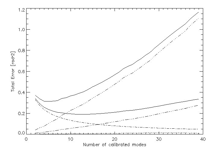
Figure 19: Different errors in dependence on the number of calibrated modes. The dotted line shows the aliasing error, the dashed line shows the error due to modal cross talk, the triple dot-dashed lines show the measurement error for S/N=1 and 2, the dash-dotted line shows the fitting error, and the solid lines show the total error for S/N of 1 and 2.

Fig.19 compares these errors. The aliasing and modal cross talk are of the same order and quite small. The measurement error is shown for S/N=1 and 2. The errors due to modal cross talk and aliasing are small compared to the others. The error , however, will decrease quadratically with rising S/N. For S/N=1 the measurement error matches the fitting error at 8 calibrated modes. The point of best correction (minimum of solid curve) is at 5 modes. For a S/N of 2 the largest contribution arises from the fitting error for up to 16 modes. The best correction is given for 13 calibrated modes. These curves are very helpful because we are able to change the number of modes we use for reconstruction on the fly, adapting to the actual situation.

5.1 Prediction of the On Sky Performance

The errors presented in the last subsections were of static nature. To derive the full error budged we need to include the temporal errors due to finite loop bandwidth $\sigma^{2}_{band}$ and time delay $\sigma^{2}_{delay}$. These errors are given as [Hardy(1998)]

$$\sigma^{2}_{band} = \left(f_{G}\over{f_{S}}\right)^{5\over{3}}$$ (15)

$$\sigma^{2}_{delay} = 28.4\left({f_{G}\tau_{S}}\right)^{5\over{3}}=28.4\left({{0.427v\tau_{S}}\over{r_{0}}}\right)^{5\over{3}}$$ (16)

with

$$r_{0} = \,Coherence\,length$$

$$f_{G} = \,Greenwood\,frequency$$

$$\tau_{S} = \,Time\,delay$$

$$v = \,Averaged\,wind\,speed$$

$$f_{S} = \,Loop\,bandwidth\,\approx 1/20\,loop\,speed.$$

In the following the sum of the two temporal errors will be referred to as $\sigma^{2}_{temp}$

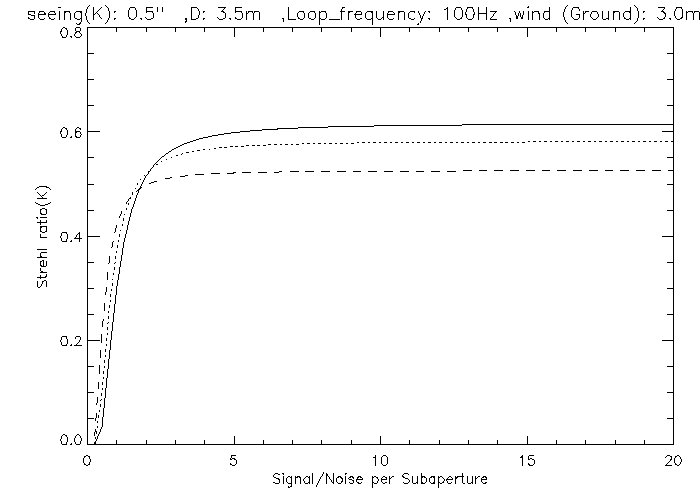
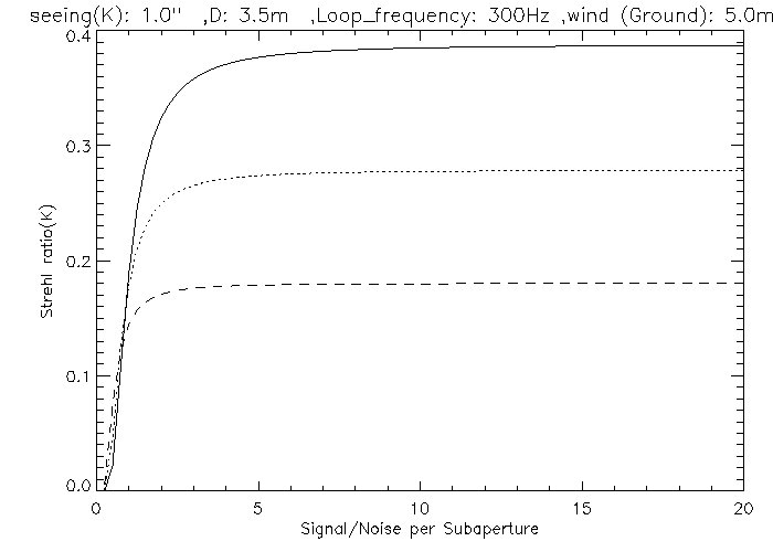
Figure 20: Left: predicted performance in K band for PYRAMIR on the sky for good seeing conditions. The three curves mark corrections with 12(dashed curve), 22(dotted curve) and 32(solid curve) modes.D denotes the telescope size, the wind speed is measured at ground level. Right: same as in the left panel, but for bad seeing conditions. Note that the bandwidth of the loop has been changed to 300 Hz. The curve styles are the same as in the left panel.

To derive the averaged wind speed from our measurements on ground level we used the 2/5 ratio between the wind speed at a height of 200m and the wind speed on ground level found on Paranal. This ratio numbers approximately 2. We adapted this factor into our model.
For the closed-loop application we also have to take into account that the cross talk amplitude is reduced with respect to the open loop case due to the correction by the system. Therefore the weighting of the cross talk is given by the residuals from aliasing, temporal error and measurement error only,

$$\sigma^{2}_{cr}\propto E_{0}^{2}(\sigma^{2}_{temp}+\sigma^{2}_{al}+\sigma^{2}_{meas})$$ (17)

The cross talk itself should occur on the right hand side also but has been omitted because in CL it is much smaller than the other errors.

Now we can derive the expected Strehl values on sky as,

$$SR=\exp[-(\sigma^{2}_{cross}+\sigma^{2}_{meas}+\sigma^{2}_{alias}+\sigma^{2}_{fit}+\sigma^{2}_{temp})]$$ (18)

Fig.20, left panel, shows the performance for a seeing of 0.5” in K-band and a wind speed on ground level of of 3 $ms^{-1}$ for a loop update rate of 100 Hz and 12, 22 and 32 modes corrected. A Strehl ratio up to about 60% is expected for bright stars. The limiting S/N is about 0.25 per subaperture. This corresponds to a stellar magnitude of 7.2 mag in K’ with 20% light on PYRAMIR.

Fig.20, right panel, shows the same for a seeing of 1” in K-band a wind speed of 5 m/s and a loop update rate of 300 Hz. Here we can still achieve about 39% Strehl ratio. The difference in performance between the number of modes in use is much more significant. The limiting signal to noise ratio is about 0.25 per subaperture. This corresponds to a magnitude of 6.0 mag in $K^{\prime}$ with 20% light on PYRAMIR. The reason the stars have to be so bright is the high sampling with 224 subapertures and the noise of 20$e^{-}$ rms per pixel.

6 Conclusions

In this article we presented laboratory measurements performed with the pyramid wavefront sensor PYRAMIR. After a short introduction into the history of PWFS and their working principles, we presented the PYRAMIR system as infrared PWFS and explained the details of the system especially the possible read out modes of the detector. This can reach a speed of about 300 Hz with a RON of 20 $e^{-}$ rms. The calibration procedure of the system was described in detail. The pitfalls of TT-calibration were discussed in detail leading to the conclusion that a static part in TT will reduce the limiting magnitude and enhance TT-jitter and cannot be tolerated. Therefore we included a static TT-part in the bias pattern of the deformable mirror (dmBias) to perfectly center the beam. Also it has to be guaranteed that the amplitudes of calibration are the same in both axis in order to gain similar performance in both directions.
Some of the fundamental sources of reduced performance were examined. We found that the amount of light diffracted out of the pupil images is 50% for a flat wavefront decreasing nonlinearly up to 2 $rad$ wavefront error where it becomes almost stable at 20%. A comparison with simulations shows that in our case this loss results from diffraction at the pyramid edges and imperfections in the optics. The latter outweighing for aberrations stronger than about 1.5 $rad$.
The effects of a Gaussian illumination of the pupils, as well as the effect of an extended calibration light source, were investigated. Both have strong influence on the sensitivity of the system and should be avoided. On the other hand an extended target during the measurement does only slightly effect the performance. Thus the calibration light source should be as point like as possible for all applications.
The effect of RON on the limiting magnitude of the guide star has been widely discussed. In the case of infrared detectors this noise is quite high. In our case 20 $e^{-}$ rms per pixel. This reduces the limiting magnitude by 5 mag. We investigated into the best possible mode set between the eigen modes of PYRAMIR, of the DM and the KL modes. The last two mode sets seem promising for the use on-sky. The latter has a larger linear regime than the eigen modes of the DM. The difference is small and, therefore, the correction error will not vary by much. Still the larger linear regime might help to close the loop under bad seeing conditions.
We tested the best treatment of noncommon-path aberrations by applying artificial modes to the DM. The best treatment turned out to direct these aberrations completely into the path of the sensor. A possible better way using two calibrations, one for modes with positive amplitude one for those with negative amplitude was proposed to reduce the error of the mode with static aberrations, but put aside due to the fact that it was not running stably during the testing on-sky.
The importance of a small calibration amplitude to minimize the resulting reconstruction error was shown.
After the measurement of these fundamental properties, the subject of the best number of modes to calibrate was addressed. To solve this we investigated into the behavior of modal cross talk, aliasing, and measurement error dependence on the number of modes calibrated. We found that the averaged aliasing coefficient varies only slightly with the number of modes whereas the average modal cross talk coefficient decreases inversely linear with this number and the measurement error rises linearly with this number. Including the (theoretical) contribution of the KL modes in the wavefront error on sky we could show that the contribution of aliasing rises like $N^{(2-\sqrt{3})\over 2}$; the contribution of cross talk becomes constant for larger $N$ and the measurement error rises linearly with $N$. In CL only the error due to modal cross talk changes with respect to the open loop measurement. It will decrease because the modes that are corrected will contribute less to the modal cross talk than in open loop. The error of the residual wavefront decreases like $N^{-{\sqrt{3}\over 2}}$. Altogether we could show that at the border of the limiting magnitude the fitting error surpasses all other errors for a low number of corrected modes but will be overpowered by the measurement error at about the place of the optimum number of modes to be corrected. For the PYRAMIR system this is 5 modes. The other errors will become important for even slightly brighter stars. Here cross talk and aliasing error are almost identical in strength. In the case of noncommon-path aberrations in the system the modal cross talk and aliasing errors will rise. Modal cross talk increases linearly, aliasing error stays constant until the static aberration reaches the border of the linear regime of the sensor, then it increases nonlinearly.
From the entire error-budged we could predict the performance on-sky for various seeing conditions. For a seeing of 1” and a wind speed on ground level of 5$ms^{-1}$ we can achieve a 39% Strehl ratio in $K^{\prime}$-band, but we have to run at about maximum frame rate (300 Hz). The limiting S/N per subaperture on the detector is about 0.25 or 6.0 mag in $K^{\prime}$. For good seeing conditions and a moderate loop band width, the predicted Strehl ratio will be about 60% for bright stars. Again the limiting S/No per subaperture on the detector is about 0.25 or 7.2 mag in $K^{\prime}$.

References

- [Campbell & Greenaway(2006)] Campbell, H.I. & Greenaway, A.H. 2006, EAS Publications series, 22, 165
- [Costa(2003)] Costa, J. 2003, PhD thesis, Ruprecht-Karls-Universiät, Heidelberg
- [Dorner(2006)] Dorner, B. 2006, Diploma thesis, Ruprecht-Karls-Universiät, Heidelberg
- [Hardy(1998)] Hardy, J. W. 1998, Oxford University Press, New York
- [Peter et al.(2006)] Peter, D. et al. 2006, SPIE, 6272, 67
- [Peter et al.(2008)] Peter, D. et al. 2008, in prep.
- [Ragazzoni & Farinato (1999)] Ragazzoni, R. & Farinato, J. 1999, A&A, 350, L23
- [Verinaud(2004)] Verinaud, C. 2004, Opt.Comm., 233, 27