Local temperature in quantum thermal states

Abstract

We consider blocks of quantum spins in a chain at thermal equilibrium, focusing on their properties from a thermodynamical perspective. In a classical system the temperature behaves as an intensive magnitude, above a certain block size, regardless the actual value of the temperature itself. However, a deviation from this behavior is expected in quantum systems. In particular, we see that under some conditions the description of the blocks as thermal states with the same global temperature as the whole chain fails. We analyze this issue by employing the quantum fidelity as a figure of merit, singling out in detail the departure from the classical behavior. As it may be expected, we see that quantum features are more prominent at low temperatures and are affected by the presence of zero-temperature quantum phase transitions. Interestingly, we show that the blocks can be considered indeed as thermal states with a high fidelity, provided an effective local temperature is properly identified. Such a result may originate from typical properties of reduced sub-systems of energy-constrained Hilbert spaces. Finally, the relation between local and global temperature is analyzed as a function of the size of the blocks and the system parameters.

I Introduction

Since the early days of quantum theory, there has been a considerable effort to formulate the principles of thermodynamics from a quantum perspective MahlerBook . Recently, this approach has allowed to discover novel features of the nature of many-body systems, see for instance Refs. tasaki ; malPRL ; malPRE ; psw ; lebo . In particular, careful analysis of the application of thermodynamics concepts to microscopic systems have shown the appearance of purely quantum features. In such systems, thermodynamic magnitudes may indeed loose their classical properties, giving rise to peculiar dependencies on some system parameters, such as size or total energy. A striking manifestation of this is given by the temperature, a magnitude considered to be intensive in classical thermodynamics. In a quantum scenario the temperature may not be well defined, resulting in the fact that subparts of thermal states may no longer be described as thermal states with the same global temperature as the whole system. More precisely, recent studies suggest that the intensive nature of the temperature may be lost not only in dependence of the size of the system subparts, as in a classical scenario, but also changing the temperature of the global system malPRL ; malPRE . It is then a relevant question to understand under which conditions the concept of temperature offers a correct description of sub-parts of quantum thermal states.

Although the main motivation of this work comes from a fundamental point of view, studying the limits of validity of thermodynamics concepts may be relevant from a practical perspective. In fact, recent experimental progress in nano-sciences allows to access thermodynamical quantities, like temperature, at scales in which deviations from classical thermodynamics may become relevant nanotherm . For example, in Refs. mahlEPL ; HartCP it has been pointed out that the breakdown of the concept of temperature might have consequences on thermometry and might be observed in experiments with spin chain compounds.

In Refs. malPRL ; malPRE a set of conditions were established in order to assure that a large thermal system can be approximated by a set of factorized blocks, each of them described in turn by a thermal state at the same temperature as the global system. Clearly, when such an approximation is valid, local measurements performed on a block provide results compatible with the global temperature. In other words, we do meet a situation in which temperature is intensive. However, local measurements on a single block do not provide any information about the correlations with the other blocks, which are simply disregarded (traced out) in the measuring process. Therefore, the approximation in Refs. malPRL ; malPRE may be further relaxed still retrieving situations compatible with the concept of intensive temperature. As a matter of fact, one may only require that the block actually measured should be in a thermal state at the same temperature as the global one, not necessarily factorized with the rest of the system. This is the approach adopted in this work.

The aim of the present work is to consider these issues exploiting ideas and tools recently emerged from quantum information science. This approach has the advantage of giving a thorough description of the quantum systems under consideration, allowing in turn to characterize in detail the departure from the classical behavior. We consider a chain composed by $n$ spins (where $n$ can be taken in the macroscopic limit) at temperature $T$ and focus on the thermodynamical properties of a block composed by $m$ spins ($m<n$) — i.e., the reduced state obtained after tracing out $n-m$ spins. In a standard thermodynamic setting $m$ and $n$ are taken large enough such that the interactions between the block and the rest of the system may be disregarded. As a consequence, the block can be well described by a thermal state at the same temperature as the global one. However, such a picture may brake down for blocks of small size and strong interactions. As said, whereas for classical systems this breakdown has no dependence on the temperature, in quantum systems a temperature dependence arises malPRL . This is the scenario that we will consider here. To face this problem we use the quantum fidelity as a figure of merit. The latter quantifies the amount of statistical distinguishability between two quantum states and its properties have been widely studied in quantum information science NC . Recently, the fidelity has been used both as an indicator of phase transitions in spins systems zan1 ; zan2 , and to study the emergence of thermal states in contiguous blocks of some spin-system ground states olav . As shown in these works, the fidelity has revealed to be a particularly sensitive figure of merit in this framework. Here, we use it to check whether the reduced states of the spin chain under consideration can be well approximated by an $m$-particle thermal state. The sensitivity of this approach will be assessed by investigating regions in the phase space near the zero-temperature critical points.

We also relate our investigations to recent findings in the foundation of statistical mechanics – again inspired by quantum information concepts. In Refs. psw ; lebo the authors address typical properties of the reduced states obtained by tracing out a huge amount of degrees of freedom from a constrained pure system. Building on previous results on properties of quantum states in large dimensional systems HLW06 , it was shown in Ref. psw that the reduced state of a big system (including environment) satisfying an operator constraint is basically the same for almost any pure state of the system. In the particular case in which (i) the operator constraint is related to the energy of the whole system and (ii) the interaction between system and environment is small, this typical state can be shown to correspond to a canonical thermal state psw ; lebo , as already pointed out in the early days of quantum mechanics schro .

Motivated by these results we study the reduced states of the chain from a thermodynamical perspective, describing it with only a few physical magnitudes, an effective temperature in our case. In other words, we check whether the reduced states of thermal systems maintain some sort of canonical typicality. Recall that the results in Refs. psw ; lebo show that a canonical thermal state for the reduced system is obtained when the interaction energy between the considered parts is negligible. As said, here we will consider settings in which such condition is not fulfilled, hence the validity of these typicality results is by no means guaranteed. Specifically, we proceed by identifying the thermal state of $m$ particles that, subject to the local interaction inherited by the whole Hamiltonian, is closer to the actual reduced state of the whole chain. We thus define an effective local temperature (the only free parameter to adjust) that can be compared with the global temperature of the whole system. Depending on the parameters of the Hamiltonian and the subsystem size we find situations where the local temperature is no longer equal to that of the global system, in accordance with the above mentioned analysis. However, the description of the reduced states as thermal states is an extremely good approximation, as shown by the corresponding fidelity. This is remarkable since, as said, we are not in the standard conditions considered in Refs. psw ; lebo . Our results then suggest that some form of canonical typicality may still be present, even if the interaction between system and environment is not negligible. In particular, we find that below some threshold temperature the local temperature may become higher than the global one, and that the reduced states can have some finite temperature even when the global system is in the ground state. Furthermore, as one may expect, the local and global temperatures tend to coincide increasing the size of the subsystem.

The structure of the paper is the following. After introducing the systems under consideration, we calculate in Section II the fidelity between two-particle blocks and the corresponding thermal state. This allows to study the conditions under which the temperature ceases to be an intensive magnitude. Then, in Section III, we derive the local effective temperature of the two-particle blocks, as well as the fidelity of this description. The dependence of the local temperature on the size of the blocks is studied in Section IV, where blocks consisting of more than two spins are studied with the help of the Matrix Product States formalism. Finally, we summarize our results in Section V and point out some conclusive remarks.

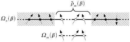
Figure 1: (Upper panel) Reduced $m$-particle state $\tilde{\rho}_{m}(\beta)$ of a chain composed by $n$ particles in the thermal state $\Omega_{n}(\beta)$ at temperature $T=1/\beta$. The state $\Omega_{n}(\beta)$ is built from an $n$-particle Hamiltonian $\hat{H}_{n}$. (Lower panel) Thermal state $\Omega_{m}(\beta)$ of $m$ particles for the same local interaction $\hat{H}_{m}$ but referred to $m$ particles.

II Intensive temperature analysis

We start by assessing the applicability of the concept of intensive temperature. As said, we consider a large spin system at temperature $T=1/\beta$ and focus on a sub-block of spins. We then check whether the latter can be well approximated by the thermal state at temperature $T$ given by the interaction inherited from the whole system Hamiltonian. By analyzing the relation between the reduced states of thermal systems and thermal states themselves, we assess the validity of such estimation.

Consider the setting depicted in Fig. 1. On the one hand, we construct the canonical state of $n$ particles $\Omega_{n}(\beta)=\exp{(-\beta\hat{H}_{n})}/Z_{n}$, where $\hat{H}_{n}$ is a local interacting Hamiltonian and $Z_{n}$ is the partition function. In order to check the thermal properties of the subparts of this state we trace out a part of it, obtaining the state of $m$ particles, $\tilde{\rho}_{m}(\beta)=Tr_{n-m}[\Omega_{n}(\beta)]$ (throughout this work we will focus on systems composed by a number of particles $n$ much larger than $m$). On the other hand, we directly construct the canonical state of $m$ particles $\Omega_{m}(\beta)=\exp{(-\beta\hat{H}_{m})}/Z_{m}$. We then compare these two density matrices using the fidelity measure notefid

$$F[\Omega_{m}(\beta),\tilde{\rho}_{m}(\beta)]=\mathrm{Tr}\left(\sqrt{\Omega}_{m}(\beta)\tilde{\rho}_{m}(\beta)\sqrt{\Omega}_{m}(\beta)\right)^{1/2}\;.$$ (1)

Throughout this Section both $\Omega_{n}(\beta)$ and $\Omega_{m}(\beta)$ are set to the same temperature, since we want to identify when the temperature is intensive.

We apply the above considerations to a 1-D spin chain characterized by the Ising Hamiltonian in a transverse field with open boundary conditions

$$\hat{H}_{n}=\frac{1}{2}\sum_{i=1}^{n-1}\sigma_{x}^{i}\otimes\sigma_{x}^{i+1}-\frac{h}{2}\sum_{i=1}^{n}\sigma_{z}^{i},$$ (2)

where $\sigma_{i}$ are the Pauli matrices, and $h$ gives the strength of an external magnetic field. The system experiences a quantum – i.e., zero temperature – phase transition when $h=h_{c}=1$ sachdev . The two-spin correlation functions are given by barouch ; nielsen

$$\langle\sigma_{x}^{i}\sigma_{x}^{i+r}\rangle =\begin{vmatrix}G_{-1}&G_{-2}&\cdots&G_{-r}&\\ G_{0}&G_{-1}&\cdots&G_{-r+1}&\\ \vdots&\vdots&\ddots&\vdots&\\ G_{r-2}&G_{r-3}&\cdots&G_{-1}&\end{vmatrix},$$ (3)

$$\langle\sigma_{y}^{i}\sigma_{y}^{i+r}\rangle =\begin{vmatrix}G_{1}&G_{0}&\cdots&G_{-r+2}&\\ G_{2}&G_{1}&\cdots&G_{-r+3}&\\ \vdots&\vdots&\ddots&\vdots&\\ G_{r}&G_{r-1}&\cdots&G_{1}&\end{vmatrix},$$ (4)

$$\langle\sigma_{z}^{i}\sigma_{z}^{i+r}\rangle =4\langle\sigma_{z}\rangle^{2}-G_{r}G_{-r},$$ (5)

where

$$G_{r}= -\frac{1}{\pi}\int_{0}^{\pi}d\phi\,\cos(\phi r)(\cos\phi-h)\frac{\tanh(\frac{1}{2}\beta\omega_{\phi})}{\omega_{\phi}}$$

$$+\frac{1}{\pi}\int_{0}^{\pi}d\phi\,\sin(\phi r)\sin(\phi)\frac{\tanh(\frac{1}{2}\beta\omega_{\phi})}{\omega_{\phi}},$$ (6)

$$\omega_{\phi}= \sqrt{(\sin\phi)^{2}+(h-\cos\phi)^{2}}.$$ (7)

The parameter $r$ sets the distance between the particles, e.g. $r=1$ means two neighbor particles. These correlators are calculated for chains in the thermodynamic limit (i.e., $n\rightarrow\infty$). Using these formulae, one can compute the reduced density matrix for the 2-spin system $\tilde{\rho}_{2}(\beta)$,

$$\tilde{\rho}_{2}(\beta)=\frac{1}{4}\left[\mathbb{I}+\sum_{i,j}\langle\sigma_{i}^{k}\sigma_{j}^{k+1}\rangle\sigma_{i}\otimes\sigma_{j}\right],$$ (8)

without the explicit construction of the global thermal state of $n$ particles nielsen .

The minimal size for which both the terms in the Hamiltonian (2) contribute to the construction of $\Omega_{m}(\beta)$ is for $m=2$. We then devote much attention to this first non-trivial case of two-spin blocks. Furthermore, it is reasonable to expect that, if for such small blocks the temperature is intensive, it will be intensive for larger blocks as well. This intuition will be confirmed in Section IV, where the size dependence of our considerations will be analyzed.

Before proceeding with the results, let us comment about our choice of the local Hamiltonian $\hat{H}_{2}$, from which the reference state $\Omega_{2}(\beta)$ is derived. With this choice we are at first sight disregarding the interaction between the $2$-spin block and the rest of the system. Whereas this may be easily justified in the case of large $m$ and $n$, it deserves to be clarified in our setting. In fact, we considered various strategies in order to take into account the interactions at the border of the block, in particular a mean-field approach, and the limit of high temperatures.

First, one may add to $\hat{H}_{2}$ a correction term which takes into account the surrounding spins of the block following a mean-field approach. The idea is to replace the operators at the boundaries by their mean value $\langle\sigma_{x}\rangle$, so the corresponding effective two-particle Hamiltonian reads

$$\hat{H}^{\prime}_{2} = \frac{1}{2}\sigma_{x}\otimes\sigma_{x}-\frac{h}{2}\sum_{i=1}^{2}\sigma_{z}^{i}+\frac{1}{2}\sum_{i=1}^{2}\langle\sigma_{x}\rangle\sigma_{x}^{i}$$ (9)

The boundary correction term however turns out be zero for any finite temperature, as $\langle\sigma_{x}\rangle=0$. This can be seen by considering that the canonical distribution $\Omega_{n}(\beta)$ inherits the symmetries of the Ising Hamiltonian, in particular the global spin-flip symmetry $U=\bigotimes_{i}\sigma_{z}^{i}$. As a consequence, one has that $[U,\Omega_{n}(\beta)]=0$, which implies that

$$[\sigma_{z},\tilde{\rho}_{1}(\beta)]=0$$ (10)

for any finite $\beta$. Considering now that $\tilde{\rho}_{1}(\beta)$ can be expanded in terms of the Pauli matrices, Eq. (10) imposes that $\langle\sigma_{x}\rangle=0$ for any $T>0$ (see also Ref. nielsen ). However, recall that a symmetry breaking can occur at $T=0$, resulting in $\langle\sigma_{x}\rangle\neq 0$.

Second, one could consider a correction valid for high temperatures. A first order expansion for $\beta\rightarrow 0$ immediately reveals that in this limit $\tilde{\rho}_{2}(\beta)$ is given by

$$\tilde{\rho}_{2}(\beta) \simeq \mathrm{Tr}_{n-2}\left(\frac{\mathbb{I}^{\otimes n}}{2^{n}}-\beta\hat{H}_{n}\right)$$ (11)

$$= \frac{\mathbb{I}^{\otimes 2}}{2^{2}}-\beta\hat{H}_{2}$$

since the Pauli matrices appearing in the interacting terms of $\hat{H}_{n}$ are traceless. The expression above for $\tilde{\rho}_{2}(\beta)$ coincides with the high-T expansion of $\Omega_{2}(\beta)$. In other words, for high temperatures the standard situation is retrieved, and no correction has to be taken into account.

In order to further clarify our choice of the local Hamiltonian, let us consider the classical antiferromagnetic one-dimensional Ising model, given by:

$$H_{n}^{\rm cl}=\sum_{i=1}^{n-1}s^{i}s^{i+1}\;,$$ (12)

where $s^{i}=\pm 1$. Notice that the model above gives the classical limit of $\hat{H}_{n}$ for the case $h=0$ note0 . It is worthwhile to briefly consider this example since it gives a relevant classical model whose local Hamiltonian contains no correction due to the boundary terms. To show this, let us consider the thermal state associated to Hamiltonian (12), described by a thermal probability distribution:

$$P(s^{1},...,s^{n})=\frac{1}{Z_{n}}\exp\left[-\beta H_{n}^{\rm cl}\right]\;,$$ (13)

where $Z_{n}$ is the partition function. A straightforward calculation shows that, by summing over all the possible configuration of the $n-2$ spins surrounding an arbitrary $2$ spin block, one obtains the following distribution function:

$$P(s^{k},s^{k+1})=\frac{1}{Z_{2}}\exp\left[-\beta H_{2}^{\rm cl}\right]\;,$$ (14)

where $k$ is arbitrary ($1<k<n$), $H_{2}^{\rm cl}=s^{k}s^{k+1}$ is the local Hamiltonian and $Z_{2}$ its respective partition function. As said, we see that for this kind of classical system no correction due to the boundary terms is expected. Furthermore, notice that Eq. (14) implies that the temperature is intensive. However we should stress here that this result is not true for a generic classical system. In conclusion, given the considerations above, it seems reasonable to consider the Hamiltonian $\hat{H}_{2}$ – without any additional correction – to build the reference state $\Omega_{2}(\beta)$. We will adopt this choice throughout the paper. Finally, let us notice that the same considerations apply for any size $m$ of the block (see Sec. IV).

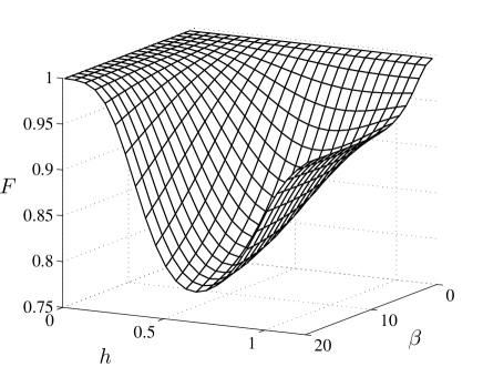
Figure 2: Fidelity $F[\Omega_{2}(\beta),\tilde{\rho}_{2}(\beta)]$ between the states $\Omega_{2}(\beta)$ (the thermal state of two spins at temperature $T=1/\beta$) and $\tilde{\rho}_{2}(\beta)$ (the two-spin reduced state of a global thermal system at temperature $T$) as a function of $\beta$ and the local magnetic field $h$ of the Ising Hamiltonian (2). The temperature ceases to be an intensive magnitude when the fidelity is significantly different from one.

The results for the fidelity $F[\Omega_{2}(\beta),\tilde{\rho}_{2}(\beta)]$ are plotted in Fig. 2. We can see that it turns to be a non-trivial function of the external magnetic field $h$ and the system global temperature $T$. In particular we observe a high fidelity above a certain temperature, for any value of $h$. This confirms the intuition that for high temperatures the classical behavior should be recovered. Namely, the reduced states are well approximated by thermal states at temperature $T$. On the other hand, as we lower the temperature, the fidelity can drop to values sensibly lower than one, thus indicating that the standard thermodynamic description of the reduced state is no longer accurate. We then recover the main feature of the results given in malPRL : the validity of the concept of intensive temperature depends on the temperature itself, a behavior with no classical analogue. Thanks to the sensitivity of the fidelity measure, we can also analyze in details such a behavior, as can be seen for low temperatures. In this case, the fidelity turns to be equal to one for $h\gg 1$ and $h\ll 1$, as can be expected recalling that in both cases the ground state is factorized (all the spins are aligned along the same direction) sachdev . On the other hand, for intermediate magnetic fields, the fidelity drops to values sensibly lower than one, showing a minimum which depends on the temperature. We recall that the model in Eq. (2) has a critical point when $h_{c}=1$.

Before proceeding further, we now explicitly assess the sensitivity of the fidelity in this scenario. For this purpose we numerically evaluated the first derivative of the fidelity with respect to $h$ at fixed $\beta$. We see in Fig. 3 that, as $\beta$ increases, the maximum of the derivative gets more pronounced. This behavior reflects the fact that the changes in the ground state become sharper and sharper as the system approaches criticality. As a consequence, subparts of the system change sharply as well and the approximation of them with a thermal state becomes more sensitive to small changes of $h$. In turn, the actual value of the maximum in Fig. 3 also increases as the temperature decreases. This behavior proceeds until we reach some $\beta$, which corresponds to some effective ground state, and below which additional changes are hardly observed. This can be understood by looking at the temperature dependence in the correlators in Eq. (6). For large $\beta$, one can well approximate $\tanh(\frac{1}{2}\beta\omega_{\phi})\approx 1$, so the reduced states become almost independent of the temperature. The derived magnitudes computed from the reduced states exhibit for this reason minor changes below some temperature.

The above considerations can be extended as well to two spins separated by $r$ particles in the chain. In particular, we considered a non-contiguous block of two distant spins which we denoted by $\tilde{\rho}_{2,r}(\beta)$. We reconstruct the density matrix of such a block using again Eq. (8) and considering the explicit dependence on $r$ of the correlators [see Eq. (6)]. Clearly, it is no longer interesting now to compare $\tilde{\rho}_{2,r}(\beta)$ with $\Omega_{2}(\beta)$. A much reasonable strategy is instead to construct a thermal state $\Omega_{r+1}(\beta)$ composed by $r+1$ spins and trace out all the particles but the two extremal ones. We denoted the two-spin state so obtained as $\Omega_{2,r}(\beta)$. Then, we can compare $\Omega_{2,r}(\beta)$ and $\tilde{\rho}_{2,r}(\beta)$ by calculating the fidelity $F[\Omega_{2,r}(\beta),\tilde{\rho}_{2,r}(\beta)]$. The results for different values of $r$ are shown in Fig. 4. Clearly the fidelity is higher with respect to $r=1$. However, some qualitative features already observed in the case $r=1$ are still present for larger $r$. In particular, the fidelity turns equal to one for $h\gg 1$ and $h\ll 1$, whereas for intermediate magnetic fields it shows a minimum.

It is worth summarizing at this point the two main features disclosed by the above analysis. Namely, i) the intensive nature of the temperature depends on the global temperature of the system itself, and ii) the temperature ceases to be intensive in a limited region of the phase space, namely for intermadiate magnetic fields around the zero-$T$ critical point. As we will mention later on, we obtained similar results also in systems different from the one given by Eq. (2).

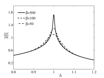
Figure 3: First derivative of the fidelity $F[\Omega_{2}(\beta),\tilde{\rho}_{2}(\beta)]$ with respect to $h$ and for fixed values of $\beta$ ($\beta=50,100,500$). The behavior turns singular at the critical point $h_{c}$ for values of $\beta$ closer to the ground state.

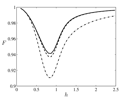
Figure 4: For fixed $\beta=10$ we plot the fidelity $F[\Omega_{2,r}(\beta),\tilde{\rho}_{2,r}(\beta)]$ between the states $\Omega_{2,r}(\beta)$ [the reduced state of two particles distant $r$ obtained from a thermal state $\Omega_{r+1}(\beta)$] and $\tilde{\rho}_{2,r}(\beta)$ [the reduced state reduced state of two particles distant $r$ obtained from a thermal state $\Omega_{n}(\beta)$ with $n\rightarrow\infty$] for $r=3,5,7$ (bottom to top). Recall that $r$ denotes the distance between two spins.

III Effective local temperature

We have seen in the preceding section that, for some values of the Hamiltonian parameters and the temperature, a two-particle block of a thermal state may be different from a two-particle thermal state under the same Hamiltonian at the same temperature. Now, we focus on the reduced state $\tilde{\rho}_{m}$ and look for a valid description of it in terms of only a few thermodynamic magnitudes. A key point in the attempt to describe the reduced states is the fact that, under some natural circumstances, they will become with high probability close to a thermal state psw ; lebo . This follows from the general structure of the Hilbert space of the global system, and the restriction over the total energy note1 . In this direction, the results in Refs. psw ; lebo are quite general but their application to a specific system has to be taken cautiously. In particular, a thermal state is recovered when the interaction between the parts of the system under consideration is negligible with respect to the interactions inside the parts themselves. This condition, however, may not always be satisfied. When the parts taken into account are composed of two spins only, as analyzed in the previous section, it is then non trivial that the reduced states are actually in a thermal state of their respective Hamiltonian. Nonetheless, we will see that this is indeed the case in the majority of the circumstances.

Following these considerations we check whether the reduced state is a thermal state as well, but at an effective local temperature different from the one of the global system. That is, even if the temperature may not be intensive, the reduced states may still have a simple thermodynamical description. To this end, we consider a generic $m$-particle thermal state $\Omega_{m}(\beta^{\prime})$ and look for the effective optimal temperature $\tilde{\beta}$ for which such a state better describes the actual $m$-particle reduced state $\tilde{\rho}_{m}(\beta)$. As outlined in the previous Section, we assume that the local interaction $\hat{H}_{m}$ is the same as in the global system $\hat{H}_{n}$ (actually $\hat{H}_{m}$ is obtained from $\hat{H}_{n}$ by tracing out the $n-m$ disregarded spins), we only have to adjust the temperature. In order to check the quality of this description, we compute the fidelity between the reduced state and the reference thermal state, and then optimize the temperature of the latter. That is, once we compute the traced state $\tilde{\rho}_{m}(\beta)$ for any given $\beta$, we optimize over the parameter $\beta^{\prime}$ the fidelity function $F[\Omega_{m}(\beta^{\prime}),\tilde{\rho}_{m}(\beta)]$. In this way, as said, we identify an effective local temperature $\beta^{\prime}=\tilde{\beta}$ for the reduced state of the system.

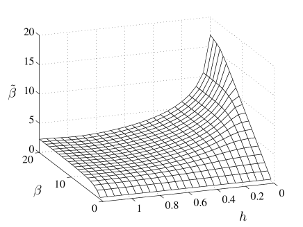
Figure 5: The optimized inverse temperature $\tilde{\beta}$ (local temperature) of a reduced subsystem of two spins as a function of $\beta$ ($\beta=1/T$, where $T$ is the global temperature of the system), for different values of $h$.

Operating similarly as in the preceding section, we study for $m=2$ the relation between $\beta$ and $\tilde{\beta}$. As shown in Fig. 5, we have that $\tilde{\beta}\approx\beta$ for low values of $\beta$ (i.e., the local temperature is the same as the global one). Thus, this range of temperatures can be identified as a classical regime, where both the local and the global temperature coincide, and the temperature behaves as an intensive magnitude. By lowering the temperature this equality stops to hold, and the value of $\tilde{\beta}$ saturates. For even lower temperatures of the global system, the reduced state keeps the same effective temperature, even in conditions of zero-$T$ where the whole chain is in its ground state. As above, this is due to the fact that for sufficiently small $T$, the reduced states hardly change with temperature. Notice also that the relation $\tilde{\beta}\approx\beta$ holds even for small temperature when the magnetic field vanishes (i.e., $h\ll 1$). This is true also for $h\gg 1$ (not shown in the picture) and can be understood in view of the considerations made in the previous Section.

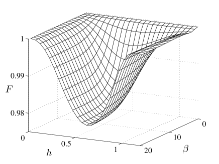
Figure 6: Optimized fidelity $F_{\rm opt}=F[\Omega_{2}(\tilde{\beta}),\tilde{\rho}_{2}(\beta)]$ between the thermal state $\Omega_{2}(\tilde{\beta})$ at an optimized inverse temperature $\tilde{\beta}$ (local temperature) and the reduced state $\tilde{\rho}_{2}(\beta)$ of two spins at inverse temperature $\beta$ (global temperature). Compared with Fig. 2 the values of the fidelity are sensibly higher.

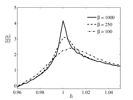
Figure 7: Value of $\frac{\partial\tilde{\beta}(\beta)}{\partial h}$ as a function of the local field $h$ ($\beta=100,250,1000$).

Performing the optimization over the local temperature we improved dramatically the previous values of the fidelity, as can be seen comparing Figs. 2 and 6 notefid2 . As a matter of fact, after the local optimization the fidelity is everywhere almost one, attaining the minimum of $F[\Omega_{2}(\tilde{\beta}),\tilde{\rho}_{2}(\beta)]\approx 0.975$ for $h\approx 0.6$. Such result implies that a local temperature $\tilde{\beta}$ may be defined for almost every $\beta$ and $h$, even if such local temperature is no longer intensive. In other words, the findings in Refs. psw ; lebo can be applied, at least approximately, also in cases like the one studied here. This is in a sense surprising, since here the assumptions used to derived the results of Refs. psw ; lebo are no longer satisfied. In particular, the block we are considering is composed by only two particles, implying that the interaction between it and the rest of the system cannot be disregarded a priori. Let us notice moreover that the definition of a local temperature is not completely satisfactory for intermediate magnetic field $h$ at low temperature. This resembles the results obtained in the previous Section even if, as said, the fidelity here obtained is much higher. We will commment on this in Sec. V.

In order to check the sensitivity of the local temperature $\tilde{\beta}$ to small changes of the parameters we studied the derivative $\frac{\partial\tilde{\beta}(\beta)}{\partial h}$ as a function of the local field $h$ which drives the quantum phase transition. We plot the results in Fig. 7, where a singular value around the critical point appears. This shows that minor changes in the global temperature will strongly change the local thermal properties of the reduced subsystem. The comparison of Fig. 3 and 7 shows that the influence at finite $T$ of the quantum phase transition is more pronounced for local effective temperatures.

We complete the study of two-particle reduced states comparing two of them at slightly different temperatures. In particular, we compute the fidelity $F[\tilde{\rho}_{2}(\beta),\tilde{\rho}_{2}(\beta+\Delta\beta)]$ between two reduced states at temperatures $\beta$ and $\beta+\Delta\beta$, as a function of the global system temperature $\beta$. Here $\tilde{\rho}_{2}(\beta)$ is again a two-particle reduced state of a chain at global temperature $\beta$. In Fig. 8 we show the fidelity as a function of $\beta$ for different values of $\Delta\beta$. The value of $\beta$ for which $F[\tilde{\rho}_{2}(\beta),\tilde{\rho}_{2}(\beta+\Delta\beta)]=1$, combined with the preceding results, suggest that above a given $\beta$ the states are equal and independent of the temperature. This is a direct indication of the asymptotic character of the reduced states $\tilde{\rho}_{2}(\beta)$ for low temperatures, as already expected from Eq. (6). In addition, the values of the fidelity for different $\Delta\beta$ appear converging to one at a value $\beta$ consistent with the saturation of the local temperature found in this Section.

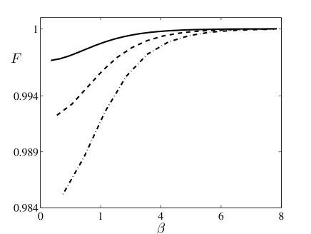
Figure 8: Fidelity $F[\tilde{\rho}_{2}(\beta),\tilde{\rho}_{2}(\beta+\Delta\beta)]$ between the two reduced states of a system at inverse temperature $\beta$ and $\beta+\Delta\beta$ respectively ($\Delta\beta=0.3,0.5,0.7$ from top to bottom). The magnetic field is set to $h=0.1$.

IV Analysis for increasing block size

In the previous Sections we mainly discussed reduced blocks consisting of two spins, not necessarily contiguous. Now, we extend our considerations to larger blocks. Recall that in the case of two-particle blocks we considered the whole system in the thermodynamic limit ($n\rightarrow\infty$) and were able to construct the density matrix of the block via the two-body correlators in Eqs. (3)-(5). Even if such a procedure can be in principle extended to higher order correlators (for the 3-spin correlators see for instance patane ), it is more convenient to use a different strategy when blocks of arbitrary length are considered. Specifically, we use the formalism of Matrix Product States (MPS), a numerical tool which has been shown to describe with high precision ground and thermal states of 1D local Hamiltonians. Using the MPS formalism for mixed states mpdo ; vidal we construct thermal states and compute correlation functions in an efficient way. Within the adopted numerical approach, we cannot work directly in the thermodynamical limit. However, the MPS formalism allows to simulate systems large enough to accurately reproduce the thermodynamical limit. We checked that systems composed by around $50$ spins already suffice to obtain results indistinguishable to the corresponding ones in the thermodynamical limit. We will explicitly show in the following such a comparison.

The interest in considering blocks of increasing size is motivated by the following observations. On the one hand, when the block increases in size the interaction between the latter and the rest of the system becomes less relevant when compared with the interactions inside the block itself. This may intuitively lead to guess that the rest of the system plays a negligible role in the thermalization process. In other words, each block in which the global system may be divided could be considered as a system on its own, thus thermalizing with the global environment independently from the rest. In such a scenario the temperature would clearly be intensive, for large enough block size. On the other hand, there are situations in which it is not possible to disregard any part of the whole system, in particular when the latter is in a highly correlated state (e.g., near a phase transition). Thus, an analysis of the intensive nature of temperature as a function of the system size can identify which of these two tendencies prevails and in which setting.

Before proceeding, let us briefly recall the MPS formalism (see mpdo for more details). This representation is based on a set of matrices $A_{k}^{s}$ of size $D\times D$ used to write a quantum state as

$$|\Psi_{MPS}\rangle=\sum_{s_{1}\ldots s_{n}=1}^{d}Tr(A_{1}^{s_{1}}\ldots A_{n}^{s_{n}})|s_{1}\ldots s_{n}\rangle.$$ (15)

We can write mixed states in the MPS formalism introducing at each position an ancillary system $a_{k}$ of dimension $d$. Thus, the thermal state $\rho$ is written as a pure state in a Hilbert space of larger dimension as

$$|\rho\rangle=\sum_{s_{1}\ldots s_{n}}^{d}\sum_{a_{1}\ldots a_{n}}^{d}Tr(\prod_{k=1}^{n}A_{k}^{s_{k},a_{k}})|s_{1}\ldots s_{n}\rangle|a_{1}\ldots a_{n}\rangle.$$ (16)

Using this purification one can recover the thermal state tracing out the ancillary systems $a_{k}$, $\rho=\mathrm{Tr}_{a}(|\rho\rangle\langle\rho|)$.

With this representation we can compute expectation values efficiently using the relation

$$\langle O_{1}\ldots O_{n}\rangle_{\rho}=Tr(E_{1,O_{1}}\ldots E_{n,O_{n}})\,,$$ (17)

where $E_{k,O}=\sum_{s,s^{\prime}}\langle s^{\prime}|O|s\rangle M_{k}^{s,s^{\prime}}$, and the set of matrices $M_{k}$ are the result of tracing the ancilla states

$$M_{k}^{s,s^{\prime}}=\sum_{a=1}^{d}A_{k}^{s,a}\otimes(A_{k}^{s^{\prime},a})^{*}\,.$$ (18)

With an initial MPS representation of a state at $\beta=0$, which corresponds to the completely mixed state 11, we obtain the state $\rho\propto\exp(-\beta H)$ using

$$e^{-\beta H}=(e^{-\Delta tH})^{M}\leavevmode\hbox{\small 1\normalsize\kern-3.30002pt1}(e^{-\Delta tH})^{M},$$ (19)

where $\Delta t=\beta/2M$. In this way the thermal state at temperature $\beta$ is the result of the evolution in imaginary time of the completely mixed state, an evolution that can also be performed in an efficient way by means of a Trotter decomposition of the time evolution operator. Using this numerical technique we can extend the calculation of the correlation functions up to $m=6$, the computational limit being the construction of the state $\rho$ from the corresponding correlators as in Eq. (8).

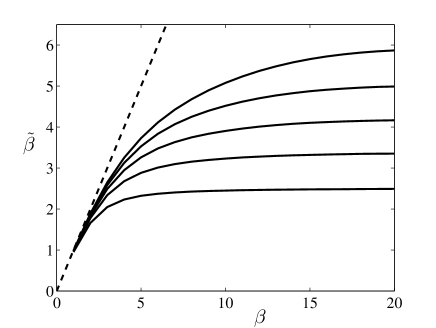
Figure 9: The local inverse temperature $\tilde{\beta}$ of a reduced subsystem of $m$ spins as a function of the global inverse temperature $\beta$ of the system (the magnetic field is set to $h=0.8$; the matrices size for the MPS algorithm is set to $D=15$). From bottom to top we set $m=2,3,4,5,6$. The dashed-dotted line shows $\beta=\tilde{\beta}$ for reference. We see that for larger blocks the local temperature gets closer to the global one. The actual region in which the temperature is intensive does not seem to be affected by the size of the block ($m>2$).

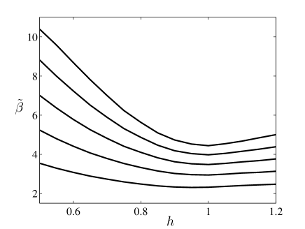
Figure 10: We plot the local inverse temperature $\tilde{\beta}$ reached by the reduced subsystem of $m$ spins as a function of the magnetic field $h$ (the global inverse temperature is set to $\beta=15$). From bottom to top the size of the block increases ($m=2,3,4,5,6$).

We plot in Fig. 9 the effective local temperature, $\tilde{\beta}$, as a function of global one, $\beta$, for reduced systems of size $m=2-6$. The first feature that one may note is that the local optimized temperature tends to get closer to the global one as the block size increases. This is in agreement with the trivial fact that for large block size the local and global temperature coincide, as the block itself coincides with the whole system. Furthermore, as mentioned above, as the block size increases the interaction between the latter and the rest of the system becomes less relevant. Thus, the block will be in a thermal state with high probability, as a consequence of the results exposed in Refs. psw ; lebo . For each curve depicted in Fig. 9, we checked explicitly the fidelity between a thermal state at temperature $\tilde{\beta}$ and the actual reduced state. We obtained that, all along these curves, the fidelity is very close to one, confirming that the results in Refs. psw ; lebo can be applied to the finite systems considered here. In turn, this points to the fact that the systems are already near to the thermodynamic limit, at least for what concerns the properties of their reduced states. However, the fact that the blocks are thermal does not mean that the temperature is intensive. As said, Fig. 9 shows that the local temperature get closer to the global one for larger blocks, nevertheless the actual region in which the temperature is intensive does not seem to be much affected by the size of the blocks. This suggests that the quantum fidelity analysis reveals fine features of the systems that cannot be understood by considerations regarding only the energy balance between the various parts of the system. In particular, as mentioned above, correlations should be considered in order to clarify such a behavior.

We also notice that for each value of $m$ a different saturation value of $\tilde{\beta}$ is obtained. The latter corresponds to the effective temperature of the reduced states when the whole system is at zero $T$. Thus for the ground states of the considered systems, the temperature is clearly not intensive, as expected. On the other hand, for high enough temperature, we can identify again a classical regime — i.e., a regime in which the temperature is intensive. In general, outside this classical region we observe that the local temperature is sensibly higher than the global one.

Before concluding this Section let us consider the influence of the zero-$T$ properties of the system at small temperatures. As seen in the previous Section (see Fig. 7), we expect that at small temperatures the features of the system ground state can be revealed by an analysis of the local temperature as a function of the local field $h$. The results for $\beta=15$ are plotted in Fig. 10. In accordance with the results reported in Fig. 9, as the block size increases the local temperature gets closer to the global ones for any value of $h$. Furthermore, notice that, as the block size increases, the minimum of $\tilde{\beta}$ (that identifies when the temperature deviates mostly from an intensive behavior) get closer to $h_{c}$. This behavior around the critical value of the field $h=1$ suggests that zero-$T$ properties of the system ground state have an important influence on the thermal state of the block.

V Conclusions

With the study of many-body systems using thermodynamic quantities, one may obtain global properties of a system by measurements performed only on a local (reduced) part of it. However, depending on the conditions of the physical system under consideration, some of the fundamental assumptions of statistical equilibrium may fail and a valid thermodynamical description cannot be possible. We have identified this situation in spin chains at low temperatures, where the reduced states are not thermal states at the same temperature as the global system. In particular, we have seen that the temperature ceases to be an intensive magnitude in dependence of the global temperature itself, a feature without classical analogue. This result is in accordance with the findings reported in Ref. malPRL . Notice, however, that here we made no assumption on the correlations between the blocks in which the global system may be decomposed. In fact, we focused only on the reduced local state of the system. Our approach is motivated by an operational viewpoint, since an actual measure performed on a local part of a system gives no information about correlations with other parts of it.

Remarkably, we have seen that an effective thermodynamical description of the reduced states is often still possible, despite the temperature may not be an intensive magnitude. In particular, the resulting reduced states can be described with high accuracy as thermal states at an optimized temperature. Interestingly, this is valid i) without any additional assumption on the interactions, and ii) even if we considered blocks of particularly small size (i.e., composed of $2$ to $6$ spins). This local temperature becomes of course equal to the global one in the regime of high temperatures, where we recover the classical behavior. However, by lowering the temperature of the global system, the local temperature saturates at some point. In other words, depending on the system parameters, the local temperature may be different from zero even when the global system is in the ground state. The dependence of the local temperature on the size of the blocks has been studied too. As one may expect, the local temperature get closer to the global one for larger blocks.

We pointed out that the departure from the classical behavior is more pronounced at low temperatures and for intermediate values of the local magnetic field, around the zero-$T$ critical point (this is true concerning both the intensive behavior of temperature and the definition of a local temperature, as can be seen in Figs. 2, 4, and 6). Notice that this is the region of parameters where quantum correlations are expected to be stronger. For example, at zero temperature the pair-wise entanglement between two spins shows its higher values in this region qpt ; nielsen , as well as the entanglement between a block of spins and the rest latorre . Though the existence of a finite block entropy may suggest that entanglement plays a crucial role in all these results, preliminary studies indicate that the relation between quantum correlations and the definition of a local temperature is nontrivial. Thus it will be a subject of further studies the way in which quantum and classical correlations lead to the bahaviours identified here.

Let us mention here that we have analyzed also other Hamiltonian systems. In this paper we have shown a study of the transverse Ising model, but the extension to a generic XY interaction leads to similar results and conclusions. Applying the MPS techniques we can extend the analysis to spin models with arbitrary interaction, such as spin chains with Heisenberg interaction. Furthermore, we analyzed chains consisting of harmonic oscillators with quadratic interaction (harmonic chains). In all these cases, the obtained results were qualitatively very similar to those shown here.

In order to assess the canonical character of the reduced states we employed the quantum fidelity, a quantity extensively used in quantum information science. We have seen that the fidelity is particularly suitable when studying the limits of applicability of the concept of intensive temperature. In particular, harnessing the sensitivity of quantum fidelity, we have observed how the low temperature features of the systems influence our results. This suggests that the quantum fidelity analysis reveals fine features of the systems that cannot be understood by considerations regarding only the energy balance between the various parts of the system. In particular, as said, future investigations should consider the role of correlations in order to clarify such a behavior.

- (1) For an historical introduction see J. Gemmer, M. Michel, and G. Mahler, Quantum Thermodynamics (Spinger, New York, 2004), and references therein.
- (2) H. Tasaki, Phys. Rev. Lett. 80, 1373 (1998).
- (3) M. Hartmann, G. Mahler and O. Hess, Phys. Rev. Lett. 93, 080402 (2004).
- (4) M. Hartmann, G. Mahler and O. Hess, Phys. Rev. E 70, 066148 (2004).
- (5) S. Popescu, A. J. Short and A. Winter, Nature Physics 2, 754 (2006).
- (6) S. Goldstein, J. L. Lebowitz, R. Tumulka and N. Zanghì, Phys. Rev. Lett. 96, 050403 (2006).
- (7) Y. Gao and Y. Bandao, Nature (London) 415, 599 (2002).
- (8) M. Hartmann and G. Mahler, Europhys. Lett. 70, 579 (2005).
- (9) M. Hartmann, Contemporary Physics 47, 89 (2006).
- (10) M. A. Nielsen and I. L. Chuang, Quantum Computation and Quantum Information (Cambridge University Press, Cambridge, UK, 2000).
- (11) P. Zanardi, H. T. Quan, X. Wang and C. P. Sun, Phys. Rev. A 75, 032109 (2007).
- (12) P. Zanardi and N. Paunkovic, Phys. Rev. E 74, 031123 (2006).
- (13) S. O. Skrøvseth, Europhys. Lett. 76, 1179 (2006).
- (14) P. Hayden, D.W. Leung, and A. Winter, Commun. Math. Phys. 265, 95 (2006).
- (15) E. Schrödinger, Statistichal Thermodynamics, Dover Publications (1989).
- (16) In this work, we take as measure of distance between two quantum states the Uhlmann fidelity, defined as . We stress that other measurements of proximity between states, such as the fidelity functions derived from the trace distance, , or the Hilbert-Shmidt distance , or the relative entropy , lead to the same main results.
- (17) S. Sachdev, Quantum Phase Transitions (Cambridge University Press, Cambridge, 1999).
- (18) E. Barouch, B. McCoy and M. Dresden, Phys. Rev. A 2, 1075 (1970); E. Barouch and B. McCoy, Phys. Rev. A 3, 786 (1971).
- (19) T.J. Osborne and M.A. Nielsen, Phys. Rev. A 66, 032110 (2002).
- (20) We are omitting the local terms since we focus on possible corrections due to interactions at the boundary of the considered block. In this case (i.e., ) the model presented in Eq. (12) gives the classical limit of the quantum model. The classical limit of the full quantum Hamiltonian can be found in A. Cuccoli, A. Taiti, R. Vaia, and P. Verrucchi, Phys. Rev. B 76, 064405 (2007). However, the analysis of the latter goes beyond the scope of the present contribution.
- (21) Here we are not considering systems for which an exchange of particles is possible between subparts of them or between the system and its environment.
- (22) Clearly, such an improvement is of relevance only in those cases where the fidelity is significantly smaller than one. In particular, our calculations show an improvement in the fidelity also for . However, in these cases, is already almost indistinguishable from one. The improvement obtained optimizing the local temperature is then insignificant.
- (23) D. Patané , R. Fazio and L. Amico, New J. Phys. 9, 322 (2007).
- (24) F. Verstraete, J. J. García-Ripoll and J. I. Cirac, Phys. Rev. Lett 93, 207204 (2004).
- (25) M. Zwolak and G. Vidal, Phys. Rev. Lett 93, 207205 (2004).
- (26) A. Osterloh, L. Amico, G. Falci and R. Fazio, Nature 416, 608 (2002).
- (27) J. I. Latorre, E. Rico, and G. Vidal, Quant. Inf. Comput. 4, 48 (2004).