On vector analogs of the modified Volterra lattice

Abstract

Modified Volterra lattice admits two vector generalizations. One of them is studied for the first time. The zero curvature representations, Bäcklund transformations, nonlinear superposition principle and the simplest explicit solutions of soliton and breather type are presented for both vector lattices. The relations with some other integrable equations are established.

Key words: Volterra lattice, Darboux transformation, nonlinear superposition principle, zero curvature representation, symmetry.

1 Introduction

Vector equations are an important and rather well studied class of integrable system. Among others, we mention but a few works in this area [1, 2, 3] containing the examples and classification results for the vectorial systems of derivative nonlinear Schrödinger type which are in some relation to the theme of our paper. There are also several interesting results for the vector differential-difference equations, or lattices, see e.g. [4, 5], but this field seems less investigated. The aim of our work is the study of the vector lattices

$$V_{n,x}=2\langle V_{n},V_{n+1}-V_{n-1}\rangle V_{n}-\langle V_{n},V_{n}\rangle(V_{n+1}-V_{n-1}),$$ (1)

$$V_{n,x}=\langle V_{n},V_{n}\rangle(V_{n+1}-V_{n-1}),$$ (2)

which define two integrable generalizations of the very well known modified Volterra lattice. Equation (1) was introduced in [6] among the other examples of the multi-component lattices related to Jordan algebraic structures. Second lattice is considered here for the first time, up to our knowledge, despite of its more simple form.

The main tool in the study of a nonlinear integrable equation is its representation as the compatibility condition for auxiliary linear systems. In the differential-difference setting this method was developed in the classical papers [7, 8]. In our paper we restrict ourselves by the version of dressing method based on Darboux-Bäcklund transformations and their nonlinear superposition principle. The main results for the scalar lattice are given in Section 2. The main body of the paper, Sections 3, 4, contains generalizations of this method for both vector lattices (1), (2), as well as the simplest explicit solutions of soliton and breather type.

A characteristic feature of integrability is the consistency of the equation with an infinite hierarchy of other equations. In particular, Bäcklund transformations define the discrete part of this hierarchy and lead to the discrete equations on the square grid. Usually, one starts this way from the continuous equations of KdV type, however an understanding appeared recently that the lattice equations of Volterra type lead to the same result as well [9, 10, 11]. This relation has not been observed in the vector case yet, although the discrete equation related to the lattice (1) has been introduced in the paper [12], see also [13, 14, 15].

The continuous part of the picture (Section 5) is more traditional. It was observed in works of Levi [16] and Shabat, Yamilov [17] that integrable Volterra type lattices define a special kind of Bäcklund transformations for equations of nonlinear Schrödinger type. This remains valid for the vector analogs as well. The connection with a two-dimensional lattice relative to the Volterra lattice introduced by Mikhailov [18] is of interest, too. Finally, it should be noted that the approach based on the continuous symmetries is the most effective one in the classification problem of integrable equations, both continuous and discrete [19]. The complete classification of scalar Volterra type lattices was obtained by Yamilov [20] by use of the symmetry approach, see also [21, 22]. Some progress in classification of vector equations and lattices has been achieved recently [3, 23, 24, 25]. We discuss some open problems in this field in the concluding Section 6.

2 Scalar case

2.1 Zero curvature representations

The following notations for the auxiliary linear equations are used throughout the paper:

$$\Psi_{n+1}=L_{n}\Psi_{n},\quad\Psi_{n,x}=A_{n}\Psi_{n},\quad\tilde{\Psi}_{n}=M_{n}\Psi_{n}.$$ (3)

Modified Volterra lattice

$$v_{n,x}=(v^{2}_{n}+a)(v_{n+1}-v_{n-1})$$ (4)

is equivalent to the compatibility condition $L_{n,x}=A_{n+1}L_{n}-L_{n}A_{n}$ with the matrices

$$L_{n}=\begin{pmatrix}\dfrac{a}{\lambda}&v_{n}\\[10.00002pt] -v_{n}&\lambda\end{pmatrix},\quad A_{n}=\begin{pmatrix}\dfrac{a^{2}}{\lambda^{2}}+v_{n-1}v_{n}&\dfrac{a}{\lambda}v_{n}+\lambda v_{n-1}\\[10.00002pt] -\dfrac{a}{\lambda}v_{n-1}-\lambda v_{n}&\lambda^{2}+v_{n-1}v_{n}\end{pmatrix}.$$ (5)

The Darboux-Bäcklund transformation is defined by the matrix

$$M_{n}=\frac{1}{a+\mu^{2}f^{2}_{n}}\begin{pmatrix}\mu(a^{2}-\mu^{2}\lambda^{2})-a\mu(\lambda^{2}-\mu^{2})f^{2}_{n}&-(a^{2}-\mu^{4})\lambda f_{n}\\[5.0pt] (a^{2}-\mu^{4})\lambda f_{n}&a\mu(\lambda^{2}-\mu^{2})-\mu(a^{2}-\mu^{2}\lambda^{2})f^{2}_{n}\end{pmatrix}.$$ (6)

Moreover, the compatibility condition $\tilde{L}_{n}M_{n}=M_{n+1}L_{n}$ is equivalent to the pair of discrete Riccati equation for the variable $f_{n}$:

$$v_{n}=\frac{\mu f_{n+1}-af_{n}/\mu}{1+f_{n}f_{n+1}},\qquad\tilde{v}_{n}=\frac{\mu f_{n}-af_{n+1}/\mu}{1+f_{n}f_{n+1}}$$ (7)

and the condition $M_{n,x}=\tilde{A}_{n}M_{n}-M_{n}A_{n}$ completes this system with the continuous Riccati equation

$$f_{n,x}=\Bigl{(}\frac{a}{\mu}v_{n-1}+\mu v_{n}\Bigr{)}f^{2}_{n}+\Bigl{(}\frac{a^{2}}{\mu^{2}}-\mu^{2}\Bigr{)}f_{n}+\mu v_{n-1}+\frac{a}{\mu}v_{n}.$$ (8)

Notice also that the variable $f_{n}$ satisfies, in virtue of equations (7), (8), the lattice

$$f_{n,x}=\frac{(\mu^{2}+af^{2}_{n})(a+\mu^{2}f^{2}_{n})(f_{n+1}-f_{n-1})}{\mu^{2}(1+f_{n+1}f_{n})(1+f_{n}f_{n-1})}.$$ (9)

Starting from a known solution $v_{n}$ of the lattice (4) the common solution of the first equation (7) and equation (8) is constructed by the formula $f_{n}=\phi_{n}/\varphi_{n}$ where $\Psi=(\phi,\varphi)$ is a particular solution of two first equations (3) at $\lambda=\mu$. Then the second equation (7) defines the new solution $\tilde{v}_{n}$.

  

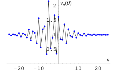
Figure 1: Breather of the lattice (4); $a=1$, $\gamma^{(1)}_{1}=\bar{\gamma}^{(2)}_{1}=0.5+1.5i$, $k^{(1)}=k^{(2)}=1$.

For example, in order to construct solutions of soliton type one takes $v_{n}=1$ as the seed solution (obviously, the choice of another constant is equivalent to scaling of parameter $a$; some generalization can be achieved via dressing of blinking solution $v_{2n}=\alpha$, $v_{2n+1}=\beta$). The eigenvalues of the matrix $L_{n}|_{v_{n}=1,\lambda=\mu}$ are defined from the equations

$$\gamma_{1}+\gamma_{2}=\mu+a/\mu,\quad\gamma_{1}\gamma_{2}=1+a$$

and the corresponding solution of the linear equations is

$$\varphi_{n}=\gamma^{n}_{1}e^{(\gamma^{2}_{1}+2)x}+k\gamma^{n}_{2}e^{(\gamma^{2}_{2}+2)x},\quad\phi_{n}=\mu\varphi_{n}-\varphi_{n+1}$$

(we do not consider the case of multiple roots $\gamma_{1}=\gamma_{2}$ which leads to rational in $n,x$ solutions). The ratio $f_{n}=\phi_{n}/\varphi_{n}$ defines the solution of the lattice (9) of kink type (provided $\gamma_{1}/\gamma_{2}>0$, $k>0$) and the substitution into the second equation (7) gives the soliton of the lattice (4). The construction of $N$-soliton solution uses the set of particular solutions $(\phi^{(j)}_{n},\varphi^{(j)}_{n})$ corresponding to the values of parameters $\mu^{(j)}$, $k^{(j)}$, $j=1,\dots,N$. If $a>0$ then the lattice (4) admits the breather solutions corresponding to the pairs of complex conjugated points in the discrete spectrum ($\mu^{(1)}=\bar{\mu}^{(2)}$, $k^{(1)}=\bar{k}^{(2)}$).

2.2 Nonlinear superposition principle

The direct recomputing of the variables $f$ is a more convenient way to iterate the Darboux transformation than applying the matrices $M$ and recomputing the wave functions. This leads to the nonlinear superposition principle of Darboux transformations in the form of some Yang-Baxter mapping [26]. Let the variables $f^{(j)}_{n}$ be constructed from the particular solutions of the linear systems at $\mu=\mu^{(j)}$, and let $f^{(j,j_{1},\dots,j_{s})}_{n}$ denote the variables obtained from $f^{(j)}_{n}$ by consequent application of Darboux transforms with parameters $\mu^{(j_{1})},\dots,\mu^{(j_{s})}$. Then the permutability of Darboux transformations is equivalent to the following equality for the matrices of the form (6):

$$M(f^{(j,k,\sigma)}_{n},\mu^{(j)})M(f^{(k,\sigma)}_{n},\mu^{(k)})=M(f^{(k,j,\sigma)}_{n},\mu^{(k)})M(f^{(j,\sigma)}_{n},\mu^{(j)})$$

where $\sigma$ stands for a tail sequence of distinct indices. This equation is uniquely solvable with respect to $f^{(j,k,\sigma)}_{n},f^{(k,j,\sigma)}_{n}$ and thus the mapping is defined

$$\binom{f^{(j,\sigma)}_{n}}{f^{(k,\sigma)}_{n}}\mapsto\binom{f^{(j,k,\sigma)}_{n}}{f^{(k,j,\sigma)}_{n}}=\binom{R(f^{(j,\sigma)}_{n},f^{(k,\sigma)}_{n};\mu^{(j)},\mu^{(k)})}{R(f^{(k,\sigma)}_{n},f^{(j,\sigma)}_{n};\mu^{(k)},\mu^{(j)})},$$

$$R(f,g;\mu,\nu)=\frac{\mu\nu^{3}(\nu g-\mu f)-a\nu(\mu^{2}-\nu^{2})fg^{2}-a^{2}(\mu g-\nu f)}{\mu\nu^{3}(\mu g-\nu f)g+a\nu(\mu^{2}-\nu^{2})-a^{2}(\nu g-\mu f)g}.$$ (10)

Another formulation of nonlinear superposition principle brings to a discrete 4-point equation on the square grid for some new variable $z^{(j,k)}_{n}$ (the subscript corresponds to the shift in the Volterra lattice and is dummy, superscripts enumerate the Darboux transformations). This equation is not too convenient for the purpose of the vector generalizations which we have in mind, however it is of interest by itself and we spend some space to describe it. The form of the equation depends on the sign of $a$.

In the simplest case $a=0$ equations (7) imply the relation

$$\frac{\mu}{\tilde{v}_{n}}-\frac{\mu}{v_{n-1}}=f_{n+1}-f_{n-1}$$

which allows to introduce the variable $z_{n}$ accordingly to the equations

$$f_{n}=\mu(\tilde{z}_{n}-z_{n-1}),\qquad 1/v_{n}=z_{n+1}-z_{n-1}.$$

This change turns the relations (7) into a single equation

$$(\tilde{z}_{n+1}-z_{n})(z_{n+1}-\tilde{z}_{n})=\mu^{-2}$$

which define Darboux transformation in terms of the variable $z$. Now, consider another Darboux transformation corresponding to the value $\lambda=\nu$:

$$(\hat{z}_{n+1}-z_{n})(z_{n+1}-\hat{z}_{n})=\nu^{-2}.$$

The easy calculation proves that the double Darboux transformations coincide: $\hat{\tilde{z}}_{n}=\tilde{\hat{z}}_{n}$ and moreover, the common value is given by the superposition formula:

$$(\hat{\tilde{z}}_{n}-z_{n})(\hat{z}_{n}-\tilde{z}_{n})=\mu^{-2}-\nu^{-2}.$$

In other words, the Darboux transformations and superposition formula form the triple which is 3D-consistent, or consistent around a cube [27]. The iterations of Darboux transformation bring to the discrete equation on the square grid (with fixed subscript)

$$(z^{(j+1,k+1)}_{n}-z^{(j,k)}_{n})(z^{(j,k+1)}_{n}-z^{(j+1,k)}_{n})=(\mu^{(j)})^{-2}-(\nu^{(k)})^{-2}.$$ (11)

This is a very well-known 3D-consistent equation which defines as well the nonlinear superposition principle of the classical Darboux transformation for Schrödinger operator. This coincidence is not too surprising since it is known for long that Volterra type lattices are symmetries of the dressing chains which define Bäcklund transformations for KdV type equations (this relation was discussed, from the different points of view, e.g. in [17, 9, 10, 11]).

Analogously, in the case $a=-c^{2}$ the variable $z_{n}$ is introduced accordingly to the formulae

$$f_{n}=\frac{\mu(\tilde{z}_{n}+z_{n-1})}{c(\tilde{z}_{n}-z_{n-1})},\qquad v_{n}=c\frac{z_{n+1}+z_{n-1}}{z_{n+1}-z_{n-1}}.$$

After this the relations (7) turn into equation

$$a(\tilde{z}_{n+1}-z_{n})(z_{n+1}-\tilde{z}_{n})=-\mu^{2}(\tilde{z}_{n+1}+z_{n})(z_{n+1}+\tilde{z}_{n}),$$

and (11) is replaced by equation

$$r(\mu^{(j)})\bigl{(}z^{(j,k)}_{n}z^{(j,k+1)}_{n}+z^{(j+1,k)}_{n}z^{(j+1,k+1)}_{n}\bigr{)}=r(\nu^{(k)})\bigl{(}z^{(j,k)}_{n}z^{(j+1,k)}_{n}+z^{(j,k+1)}_{n}z^{(j+1,k+1)}_{n}\bigr{)}$$ (12)

where $r(\lambda)=(\lambda^{2}-a)/(\lambda^{2}+a)$, which is equivalent to nonlinear superposition principle for $\sinh$-Gordon equation.

Finally, if $a=c^{2}$ then the change

$$f_{n}=\frac{\mu(1+z_{n-1}\tilde{z}_{n})}{c(z_{n-1}-\tilde{z}_{n})},\qquad v_{n}=c\frac{1+z_{n+1}z_{n-1}}{z_{n+1}-z_{n-1}}$$

is used which brings equations (7) to the form

$$a(\tilde{z}_{n+1}-z_{n})(z_{n+1}-\tilde{z}_{n})=\mu^{2}(1+\tilde{z}_{n+1}z_{n})(1+z_{n+1}\tilde{z}_{n})$$

and leads to equation

$$\begin{gathered}\bigl{(}r(\mu^{(j)})+r(\nu^{(j)})\bigr{)}\bigl{(}z^{(j,k+1)}_{n}-z^{(j+1,k)}_{n}\bigr{)}\bigl{(}z^{(j,k)}_{n}-z^{(j+1,k+1)}_{n}\bigr{)}\qquad\qquad\qquad\\ \qquad\qquad\qquad=\bigl{(}r(\mu^{(j)})-r(\nu^{(j)})\bigr{)}\bigl{(}1+z^{(j,k+1)}_{n}z^{(j+1,k)}_{n}\bigr{)}\bigl{(}1+z^{(j,k)}_{n}z^{(j+1,k+1)}_{n}\bigr{)}\end{gathered}$$ (13)

equivalent to nonlinear superposition principle for $\sin$-Gordon equation. Equation (12) turns into (13) under the complex change $z\to(i-z)/(i+z)$, so that these equations are two different real forms of one and the same equation.

Concluding this Section, we notice that an analogous construction scheme exists also for solutions of the Volterra lattice

$$u_{n,x}=u_{n}(u_{n+1}-u_{n-1}).$$

The corresponding formulae are even much simpler, for example the equations

$$u_{n}=(v_{n}-\mu)(v_{n+1}+\mu),\quad\tilde{u}_{n}=(v_{n+1}-\mu)(v_{n}+\mu)$$

replaces (7) while the role of the lattice (9) is played by the lattice (4) at $a=-\mu^{2}$. Therefore, the lattice (9) is actually the second modification of Volterra lattice. This sequence is analogous to the sequence of equations KdV $\to$ mKdV $\to$ $\exp$-CD which can be obtained by continuous limit from the lattices under consideration. Unfortunately, although the Volterra lattice admits some multi-component generalizations [28, 29], the vector ones are absent, this is why we have started from the more complicated object.

3 First vector generalization

Sometimes the zero curvature representation for a vector generalization can be obtained just by passing to the block matrices. Unfortunately, this is not the case for the matrices (5), (6). It turns out, however, that such block generalization is easy if one consider the linear equations for the length 3 vector with the components consisting of the products of the components of $\Psi$. Additionally, it is convenient to apply a gauge transformation in order to make the determinants of the matrices $L,M$ constant and the matrix $A$ traceless. In this way we come to the following matrices which define, as can be easily verified, the zero curvature representation for the lattice (4) at $a=0$ and its Bäcklund transformation:

$$L_{n}=\begin{pmatrix}0&0&1\\[6.99997pt] 0&-1&\dfrac{\lambda}{v_{n}}\\[10.00002pt] 1&-\dfrac{2\lambda}{v_{n}}&\dfrac{\lambda^{2}}{v^{2}_{n}}\end{pmatrix},\qquad M_{n}=\begin{pmatrix}\dfrac{\lambda^{2}}{\mu^{2}f^{2}_{n}}&-\dfrac{2\lambda}{\mu f_{n}}&1\\[10.00002pt] \dfrac{\lambda}{\mu f_{n}}&-1-\dfrac{\lambda^{2}}{\mu^{2}}&\dfrac{\lambda f_{n}}{\mu}\\[10.00002pt] 1&-\dfrac{2\lambda f_{n}}{\mu}&\dfrac{\lambda^{2}f^{2}_{n}}{\mu^{2}}\end{pmatrix},$$

$$A_{n}=\lambda\begin{pmatrix}-\lambda&2v_{n-1}&0\\[5.0pt] -v_{n}&0&v_{n-1}\\[5.0pt] 0&-2v_{n}&\lambda\end{pmatrix}.$$

It is not a problem to find the matrices for the general case $a\neq 0$, but they are more cumbersome. Fortunately, we will not need them, since one of the vector lattices exists only in the case $a=0$ anyway, and for the second one this assumption does not lead to the loss of generality (see Section 4).

The block matrices for the vector lattices are derived from here under the “proper” interpretation of $v_{n}$ as a vector-valued quantity. To make notation more clear we toggle to the upper case for the vectors. We assume that the vector space is equipped with a symmetric scalar product $\langle U,V\rangle=\langle V,U\rangle$. The identity operator is denoted $I$ and the linear form $V^{\top}$, inverse vector $V^{-1}$ and operator $UV^{\top}$ are defined as follows:

$$V^{\top}(U)=\langle V,U\rangle,\qquad V^{-1}=\frac{V}{\langle V,V\rangle}\qquad UV^{\top}(W)=U\langle V,W\rangle.$$

In the case of finite-dimensional Euclidean space one can think of $V$ as of the column vector and of $V^{\top}$ as of the row vector.

The first vector analog of the lattice (4) exists only at $a=0$. It is of the form [6]

$$V_{n,x}=2\langle V_{n},V_{n+1}-V_{n-1}\rangle V_{n}-\langle V_{n},V_{n}\rangle(V_{n+1}-V_{n-1}).$$ (14)

This lattice appears as the compatibility condition for the linear systems

$$T\begin{pmatrix}\psi_{n-1}\\ \Psi_{n}\\ \psi_{n}\end{pmatrix} =\begin{pmatrix}0&0&1\\ 0&-I&\lambda V^{-1}_{n}\\ 1&-2\lambda(V^{-1}_{n})^{\top}&\lambda^{2}/\langle V_{n},V_{n}\rangle\end{pmatrix}\begin{pmatrix}\psi_{n-1}\\ \Psi_{n}\\ \psi_{n}\end{pmatrix},$$ (15)

$$D_{x}\begin{pmatrix}\psi_{n-1}\\ \Psi_{n}\\ \psi_{n}\end{pmatrix} =\lambda\begin{pmatrix}-\lambda&2V^{\top}_{n-1}&0\\ -V_{n}&0&V_{n-1}\\ 0&-2V^{\top}_{n}&\lambda\end{pmatrix}\begin{pmatrix}\psi_{n-1}\\ \Psi_{n}\\ \psi_{n}\end{pmatrix}.$$ (16)

Notice that the systems (15), (16) possess the first integral in common

$$J=\langle\Psi_{n},\Psi_{n}\rangle-\psi_{n}\psi_{n-1},\qquad(T-1)(J)=D_{x}(J)=0.$$ (17)

The Darboux transformation is defined by a particular solution at the zero level of this first integral.

Statement 1.

Let $F_{n}=\Phi_{n}/\phi_{n}$ where $\psi=\phi$, $\Psi=\Phi$ is a particular solution of the linear systems (15), (16) at $\lambda=\mu$ and at $J=0$. Then the transformation

$$\begin{pmatrix}\tilde{\psi}_{n-1}\\[2.84526pt] \tilde{\Psi}_{n}\\[2.84526pt] \tilde{\psi}_{n}\end{pmatrix}=\begin{pmatrix}\dfrac{\lambda^{2}}{\mu^{2}\langle F_{n},F_{n}\rangle}&-\dfrac{2\lambda}{\mu}(F^{-1}_{n})^{\top}&1\\ \dfrac{\lambda}{\mu}F^{-1}_{n}&\Bigl{(}\dfrac{\lambda^{2}}{\mu^{2}}-1\Bigr{)}I-\dfrac{2\lambda^{2}}{\mu^{2}}F^{-1}_{n}F^{\top}_{n}&\dfrac{\lambda}{\mu}F_{n}\\ 1&-\dfrac{2\lambda}{\mu}F^{\top}_{n}&\dfrac{\lambda^{2}}{\mu^{2}}\langle F_{n},F_{n}\rangle\end{pmatrix}\begin{pmatrix}\psi_{n-1}\\[2.84526pt] \Psi_{n}\\[2.84526pt] \psi_{n}\end{pmatrix}$$ (18)

maps the general solution of these systems into the solution of the systems of the same form, with the original and transformed potentials related by equations

$$\mu V_{n}^{-1}=F_{n}+F^{-1}_{n+1},\qquad\mu\tilde{V}^{-1}_{n}=F_{n+1}+F^{-1}_{n}.$$ (19)

The expanded form of relations (19) is

$$V_{n} =\mu\frac{F_{n+1}+\langle F_{n+1},F_{n+1}\rangle F_{n}}{1+2\langle F_{n},F_{n+1}\rangle+\langle F_{n},F_{n}\rangle\langle F_{n+1},F_{n+1}\rangle},$$ (20)

$$\tilde{V}_{n} =\mu\frac{F_{n}+\langle F_{n},F_{n}\rangle F_{n+1}}{1+2\langle F_{n},F_{n+1}\rangle+\langle F_{n},F_{n}\rangle\langle F_{n+1},F_{n+1}\rangle}.$$

Each of these transformations is the substitution to the lattice (14) from the lattice

$$F_{n,x}=\mu^{2}(F_{n-1}+F^{-1}_{n})^{-1}-\mu^{2}(F_{n+1}+F^{-1}_{n})^{-1}.$$

It is easy to see that these formulae turn into (7) and (9) in the scalar case at $a=0$.

  

  

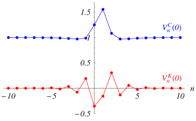
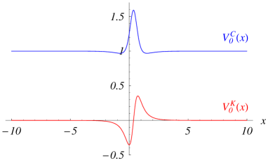
Figure 2: A soliton of the lattice (14); $C=(1,0)$, $K=(0,1)$, $\gamma=2$, $c_{1}=1$, $c_{3}=-1$.

The derivation of the nonlinear superposition principle is not more difficult than in the scalar case. One comes by multiplying the matrices $M$ of the form (18) to the following Yang-Baxter mapping (cf eq. (10) at $a=0$)

$$F^{(j,k,\sigma)}_{n}=R(F^{(j,\sigma)}_{n},F^{(k,\sigma)}_{n};\mu^{(j)},\mu^{(k)}),\qquad F^{(k,j,\sigma)}_{n}=R(F^{(k,\sigma)}_{n},F^{(j,\sigma)}_{n};\mu^{(k)},\mu^{(j)}),$$

$$R(F,G;\mu,\nu)=\frac{(\mu^{2}-\nu^{2})\langle G,G\rangle F+\mu(\nu\langle F,F\rangle-2\mu\langle F,G\rangle+\nu\langle G,G\rangle)G}{\langle G,G\rangle\langle\nu F-\mu G,\nu F-\mu G\rangle}.$$ (21)

It is possible to obtain the analog of equation (11), too. Let us introduce the new vector variable $Z_{n}$ accordingly to the formulae

$$F_{n}=\mu(\tilde{Z}_{n}-Z_{n-1}),\qquad V^{-1}_{n}=Z_{n+1}-Z_{n-1}.$$

Equations (19) become equivalent to the single equation

$$\tilde{Z}_{n+1}-Z_{n}=\mu^{-2}(Z_{n+1}-\tilde{Z}_{n})^{-1}$$

under this change. Next, consider Darboux transformation corresponding to the spectral value $\lambda=\nu$:

$$\hat{Z}_{n+1}-Z_{n}=\nu^{-2}(Z_{n+1}-\hat{Z}_{n})^{-1}.$$

The direct calculation shows that the repeated Darboux transformations coincide: $\hat{\tilde{Z}}_{n}=\tilde{\hat{Z}}_{n}$ and moreover, the result is given by the equation

$$\hat{\tilde{Z}}_{n}-Z_{n}=(\mu^{-2}-\nu^{-2})(\hat{Z}_{n}-\tilde{Z}_{n})^{-1}.$$

Iterations of the Darboux transformation are governed by the 3D-consistent discrete equation on the square grid (the subscript $n$ is dummy):

$$Z^{(j+1,k+1)}_{n}-Z^{(j,k)}_{n}=\bigl{(}(\mu^{(j)})^{-2}-(\nu^{(k)}\bigr{)}^{-2})\bigl{(}Z^{(j,k+1)}_{n}-Z^{(j+1,k)}_{n}\bigr{)}^{-1}.$$

This equation with important applications in the discrete geometry was introduced in [12] (a special reduction was considered in [15]), see also [13, 14].

  

Figure 3: A breather of the lattice (14); $C=(1,0)$, $K=(0,1)$, $\gamma^{(1)}=\bar{\gamma}^{(2)}=0.5+i$, $c^{(1)}_{1}=c^{(2)}_{1}=0.5$, $c^{(1)}_{3}=c^{(2)}_{3}=1$.

Let us make use of Darboux transformation for construction of the soliton solution. The solution of the linear equations (15), (16) with constant coefficients $V_{n}=C=\mathop{\rm const}$, $\langle C,C\rangle=1$, at $\lambda=\mu$ reads

$$\begin{gathered}\phi_{n}=c_{1}\gamma^{n}e^{(\gamma-\gamma^{-1})x}+c_{2}\gamma^{-n}e^{(\gamma^{-1}-\gamma)x}+2c_{3},\\ \Phi_{n}=(-1)^{n}K+\mu\left(\frac{c_{1}\gamma^{n}}{1+\gamma}\,e^{(\gamma-\gamma^{-1})x}+\frac{c_{2}\gamma^{-n}}{1+\gamma^{-1}}\,e^{(\gamma^{-1}-\gamma)x}+c_{3}\right)C,\\ \mu^{2}=\gamma+2+\gamma^{-1},\qquad\langle C,K\rangle=0,\qquad\gamma\langle K,K\rangle=(1-\gamma)^{2}(c_{1}c_{2}-c^{2}_{3})\end{gathered}$$ (22)

(the latter relation is equivalent to the constraint $J=0$; and we do not consider the cases of multiple eigenvalues $\mu=0$, $\mu=\pm 2$). The equations (19) bring, after elementary transformations, to the one-soliton solution of the lattice (fig. 2)

$$\tilde{V}_{n}=\frac{\phi_{n+1}\Phi_{n}+\phi_{n-1}\Phi_{n+1}}{\mu\phi^{2}_{n}}.$$

Clearly, this solution always lies in the plane of the vectors $C,K$, that is it is actually 2-component, independently on the dimension of the vector space under consideration. The $C$-component is a soliton on the unit background. Its shape is slightly different for positive and negative values of $c_{3}$. The $K$-component has localized oscillations on the zero background. They originate from the powers of $-1$ in the solution (22) rather than a pair of complex conjugated points of the discrete spectrum, that is this solution is not a genuine breather. However, the additional dimension makes the breathers possible as well, in spite of the absence of the parameter $a$ (fig. 3). The $N$-soliton solution is constructed starting from a set of solutions of the form (22) and evolves in the space spanned over the vectors $C,K^{(1)},\dots,K^{(N)}$.

4 Second vector generalization

The lattice

$$U_{n,x}=(\langle U_{n},U_{n}\rangle+a)(U_{n+1}-U_{n-1})$$ (23)

looks more natural and simple generalization of the lattice (4). In contrast with (14) it is integrable at arbitrary value of parameter $a$, though it turns out to be not so important as in the scalar case. Indeed, it can be easily eliminated or, more precisely, “confined inside the lattice” at the expense of increasing by 1 the dimension of the vector space under consideration. This is done by means of the orthogonal complement: let $U_{n}$ be a solution of the lattice (23) then the vector

$$V_{n}=U_{n}+E,\quad E=\mathop{\rm const},\quad\langle U_{n},E\rangle=0,\quad\langle E,E\rangle=a$$ (24)

(if $a<0$ then a pseudoeuclidean scalar product is used) satisfies the lattice

$$V_{n,x}=\langle V_{n},V_{n}\rangle(V_{n+1}-V_{n-1}).$$ (25)

This transformation does not lead to any problem when constructing solutions since the reduction (24) is consistent with higher symmetries and Bäcklund transformation. On the other hand, all formulae simplify essentially (cf e.g. equations (29) and (33) below). The matrices of the zero curvature representation become simpler as well.

The lattice (25) is the compatibility condition of the linear systems

$$T\begin{pmatrix}\psi_{n-1}\\ \Psi_{n}\\ \psi_{n}\end{pmatrix}=\begin{pmatrix}0&0&1\\[10.00002pt] 0&I-2V^{-1}_{n}V^{\top}_{n}&\lambda V^{-1}_{n}\\[10.00002pt] 1&-2\lambda(V^{-1}_{n})^{\top}&\lambda^{2}/\langle V_{n},V_{n}\rangle\end{pmatrix}\begin{pmatrix}\psi_{n-1}\\ \Psi_{n}\\ \psi_{n}\end{pmatrix},$$ (26)

$$D_{x}\begin{pmatrix}\psi_{n-1}\\ \Psi_{n}\\ \psi_{n}\end{pmatrix}=\begin{pmatrix}-\lambda^{2}&2\lambda V^{\top}_{n-1}&0\\[10.00002pt] -\lambda V_{n}&2V_{n}V^{\top}_{n-1}-2V_{n-1}V^{\top}_{n}&\lambda V_{n-1}\\[10.00002pt] 0&-2\lambda V^{\top}_{n}&\lambda^{2}\end{pmatrix}\begin{pmatrix}\psi_{n-1}\\ \Psi_{n}\\ \psi_{n}\end{pmatrix}.$$ (27)

These systems possess the first integral (17) in common, like in the previous case.

Statement 2.

Let $F_{n}=\Phi_{n}/\phi_{n}$ where $\psi=\phi$, $\Psi=\Phi$ is a particular solution of the linear systems (26), (27) at $\lambda=\mu$ and such that $J=\langle\Phi_{n},\Phi_{n}\rangle-\phi_{n}\phi_{n-1}=0$. Then the transform

$$\begin{pmatrix}\tilde{\psi}_{n-1}\\[2.84526pt] \tilde{\Psi}_{n}\\[2.84526pt] \tilde{\psi}_{n}\end{pmatrix}=\begin{pmatrix}\dfrac{\lambda^{2}}{\mu^{2}\langle F_{n},F_{n}\rangle}&-\dfrac{2\lambda}{\mu}(F^{-1}_{n})^{\top}&1\\ \dfrac{\lambda}{\mu}F^{-1}_{n}&\Bigl{(}1-\dfrac{\lambda^{2}}{\mu^{2}}\Bigr{)}I-2F^{-1}_{n}F^{\top}_{n}&\dfrac{\lambda}{\mu}F_{n}\\ 1&-\dfrac{2\lambda}{\mu}F^{\top}_{n}&\dfrac{\lambda^{2}}{\mu^{2}}\langle F_{n},F_{n}\rangle\end{pmatrix}\begin{pmatrix}\psi_{n-1}\\[2.84526pt] \Psi_{n}\\[2.84526pt] \psi_{n}\end{pmatrix}$$ (28)

maps the general solution of these systems into solution of the systems of the same kind, with the original and transformed potential related by the equations

$$V_{n}=\mu\frac{F_{n+1}-\langle F_{n+1},F_{n+1}\rangle F_{n}}{1-\langle F_{n},F_{n}\rangle\langle F_{n+1},F_{n+1}\rangle},\qquad\tilde{V}_{n}=\mu\frac{F_{n}-\langle F_{n},F_{n}\rangle F_{n+1}}{1-\langle F_{n},F_{n}\rangle\langle F_{n+1},F_{n+1}\rangle}.$$ (29)

In comparison with the previous Section, the equations (29) are slightly shorter than (20), but the analog of the lattice (9) is more cumbersome:

$$F_{n,x}=\frac{\mu^{2}\langle F_{n},F_{n}\rangle\bigl{(}(F_{n}-F^{-1}_{n-1})^{-1}-(F_{n}-F^{-1}_{n+1})^{-1}\bigr{)}}{\langle(F_{n}-F^{-1}_{n-1})^{-1},F_{n}+F^{-1}_{n-1}\rangle\langle(F_{n}-F^{-1}_{n+1})^{-1},F_{n}+F^{-1}_{n+1}\rangle}.$$

The superposition of Darboux transformations is defined by the Yang-Baxter map

$$F^{(j,k,\sigma)}_{n}=R(F^{(j,\sigma)}_{n},F^{(k,\sigma)}_{n};\mu^{(j)},\mu^{(k)}),\qquad F^{(k,j,\sigma)}_{n}=R(F^{(k,\sigma)}_{n},F^{(j,\sigma)}_{n};\mu^{(k)},\mu^{(j)}),$$

$$R(F,G;\mu,\nu)=\frac{(\nu^{2}-\mu^{2})\langle G,G\rangle F+\nu(\mu\langle F,F\rangle-2\nu\langle F,G\rangle+\mu\langle G,G\rangle)G}{\langle G,G\rangle\langle\nu F-\mu G,\nu F-\mu G\rangle}.$$ (30)

Notice that the formulae (21) and (30) coincide up to the permutation of $\mu$ and $\nu$ in the numerator. Despite of such similarity, an analog of equation (11) is probably lacked in this case.

Statement 3.

The Darboux transformation is consistent with the reduction (24).

Proof.

Let us apply the change $V_{n}=U_{n}+E$, $F_{n}=H_{n}+h_{n}E$, $\langle H_{n},E\rangle=0$ to the equations (29), with the scalar factor $h_{n}$ unknown for the moment:

$$U_{n}+E =\mu\frac{H_{n+1}+h_{n+1}E-(\langle H_{n+1},H_{n+1}\rangle+ah^{2}_{n+1})(H_{n}+h_{n}E)}{1-(\langle H_{n},H_{n}\rangle+ah^{2}_{n})(\langle H_{n+1},H_{n+1}\rangle+ah^{2}_{n+1})},$$ (31)

$$\tilde{U}_{n}+E =\mu\frac{H_{n}+h_{n}E-(\langle H_{n},H_{n}\rangle+ah^{2}_{n})(H_{n+1}+h_{n+1}E)}{1-(\langle H_{n},H_{n}\rangle+ah^{2}_{n})(\langle H_{n+1},H_{n+1}\rangle+ah^{2}_{n+1})}.$$

Collecting the coefficients of $E$ yields the coupled algebraic equations for $h_{n}$ and $h_{n+1}$. It is not obvious beforehand that their solution is compatible with the shift in $n$. If this would be not the case then the change $F_{n}=H_{n}+h_{n}E$ would be incorrect. However, the direct computation proves that $h_{n}$ is defined by one and the same formula for all $n$ as a solution of quadratic equation

$$ah^{2}_{n}-\mu h_{n}+\langle H_{n},H_{n}\rangle+1=0,$$ (32)

therefore the $E$-component is detached in the transformation (29). ∎

Statement 3 makes abundant the separate study of the case $a\neq 0$. Nevertheless, all formulae can be, in principle, rewritten for this case as well, moreover, their rational structure can be preserved by use of the stereographic projection for the quadric (32):

$$H_{n}=\frac{(\nu^{2}-a)F_{n}}{\nu^{2}+a\langle F_{n},F_{n}\rangle},\quad h_{n}=\frac{\nu(1+\langle F_{n},F_{n}\rangle)}{\nu^{2}+a\langle F_{n},F_{n}\rangle},\quad\mu=\nu+\frac{a}{\nu}$$

(more rigorously, some other letter should be used here instead of $F$, but we hope it will not lead to misunderstanding). For instance, the substitution into (31) brings, under this parametrization, to the Bäcklund transformation for the lattice with parameter (23):

$$U_{n} =\frac{(\nu^{2}+a\langle F_{n},F_{n}\rangle)F_{n+1}-(a+\nu^{2}\langle F_{n+1},F_{n+1}\rangle)F_{n}}{\nu(1-\langle F_{n},F_{n}\rangle\langle F_{n+1},F_{n+1}\rangle)},$$ (33)

$$\tilde{U}_{n} =\frac{(\nu^{2}+a\langle F_{n+1},F_{n+1}\rangle)F_{n}-(a+\nu^{2}\langle F_{n},F_{n}\rangle)F_{n+1}}{\nu(1-\langle F_{n},F_{n}\rangle\langle F_{n+1},F_{n+1}\rangle)}.$$

The Yang-Baxter map (30) can be rewritten in more general form in a similar way. The transformation (33) turns into (29) at $a=0$, while in the scalar case we come back to the transformation (7), under identifying $U,F,\nu$ with $v,f,\mu$ respectively.

  

  

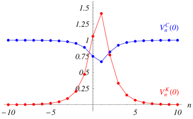
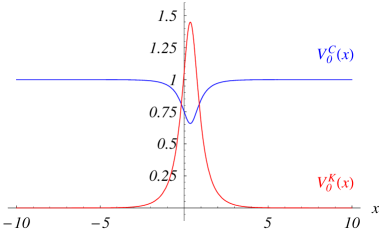
Figure 4: Solutions of the lattice (25) at $C=(1,0)$, $K=(0,1)$. Soliton: $\gamma=2$, $c_{1}=1$, $c_{3}=-1$; breather: $\gamma^{(1)}=\bar{\gamma}^{(2)}=1+1.5i$, $c^{(1)}_{1}=c^{(2)}_{1}=3$, $c^{(1)}_{3}=c^{(2)}_{3}=-1$.

It is not difficult to compute, by use of (29), the one-soliton solution

$$\tilde{V}_{n}=\mu\frac{\phi_{n+1}\Phi_{n}-\phi_{n-1}\Phi_{n+1}}{\phi_{n}(\phi_{n+1}-\phi_{n-1})},$$

where the solution $\phi_{n},\Phi_{n}$ of equations (26), (27) with constant coefficients is given by almost the same formulae (22) as before, with the only difference that the factor $(-1)^{n}$ in front of $K$ disappears. This distinction leads to the absence of blinking oscillations in the one-soliton solution which is more natural from the point of view of the continuous limit. In all other respects the construction of multisoliton and breather solutions is analogous to the previous case.

5 Higher symmetries and associated systems

Both vector lattices (14) and (25) belong to an infinite hierarchy of commuting flows. We restrict ourselves by consideration of the simplest higher symmetries which are of the second order with respect to the shift in $n$. In the scalar case one has, setting $a=0$ for simplicity, the pair of consistent lattices

$$v_{n,x}=v^{2}_{n}(v_{n+1}-v_{n-1}),\quad v_{n,t}=v^{2}_{n}(v^{2}_{n+1}(v_{n+2}+v_{n})-v^{2}_{n-1}(v_{n}+v_{n-2})).$$ (34)

Obviously, the first of these equations can be solved with respect to $v_{n+1}$ or $v_{n-1}$, and this allows to express recursively all $v_{j}$ through the pair of variables $u=v_{n+1}$, $v=v_{n}$. After this, the symmetry takes the form of Kaup-Newell evolution system

$$u_{t}=u_{xx}+(2u^{2}v)_{x},\quad v_{t}=-v_{xx}+(2uv^{2})_{x}$$

and the shift in $n$ defines an explicit auto-substitution for this system (the simplest type of Bäcklund transforms).

The lattice (14) and its symmetry can be compactly written in the form preserving the structure (34)

$$V_{n,x}=P_{V_{n}}(V_{n+1}-V_{n-1}),\quad V_{n,t}=P_{V_{n}}(P_{V_{n+1}}(V_{n+2}+V_{n})-P_{V_{n-1}}(V_{n}+V_{n-2}))$$ (35)

by use of the operator $P_{V}(U)=2\langle V,U\rangle V-\langle V,V\rangle U$. It is easy to check that the identity $(P_{V})^{-1}=P_{V^{-1}}$ is valid for this operator. Making use of it one can solve, like before, the first equation with respect to $V_{n+1}$ or $V_{n-1}$ and to express all $V_{j}$ through the pair of variables $U=V_{n+1}$, $V=V_{n}$. This brings the symmetry to the form of the vector generalization of Kaup-Newell system

$$U_{t}=U_{xx}+(4\langle U,V\rangle U-2\langle U,U\rangle V)_{x},\quad V_{t}=-V_{xx}+(4\langle U,V\rangle V-2\langle V,V\rangle U)_{x}.$$ (36)

Analogously, the commuting flows for the second vector lattice are

$$V_{n,x} =\langle V_{n},V_{n}\rangle(V_{n+1}-V_{n-1}),$$ (37)

$$V_{n,t} =\langle V_{n},V_{n}\rangle\bigl{(}\langle V_{n+1},V_{n+1}\rangle(V_{n+2}-V_{n})+\langle V_{n-1},V_{n-1}\rangle(V_{n}-V_{n-2})$$

$$\qquad+2(\langle V_{n+1},V_{n}\rangle+\langle V_{n},V_{n-1}\rangle)(V_{n+1}-V_{n-1})\bigr{)}$$

and the associated evolution system reads

$$U_{t}=U_{xx}+4\langle U,V\rangle U_{x}+2\langle U,U\rangle V_{x},\quad V_{t}=-V_{xx}+4\langle U,V\rangle V_{x}+2\langle V,V\rangle U_{x}$$ (38)

which is another vector analog of Kaup-Newell system.

Another interesting type of associated systems is obtained for the scalar quantities

$$p_{n}=\langle V_{n},V_{n}\rangle,\quad q_{n}=2\langle V_{n},V_{n-1}\rangle$$

which satisfy, in virtue of any of the pair (35) or (37) one and the same two-dimensional modified Volterra lattice

$$p_{n,t}+2p^{2}_{n}(p_{n+1}-p_{n-1})=p_{n}((q_{n+1}+q_{n})_{x}+q^{2}_{n+1}-q^{2}_{n}),\quad p_{n,x}=p_{n}(q_{n+1}-q_{n}).$$ (39)

It can be written in the form

$$p_{n,t}+2p^{2}_{n}(p_{n+1}-p_{n-1})=(r_{n}p_{n})_{x},\quad(p_{n+1}p_{n})_{x}=p_{n+1}p_{n}(r_{n+1}-r_{n}),$$

as well, where $r_{n}=q_{n+1}+q_{n}=2\langle V_{n},V_{n+1}+V_{n-1}\rangle$. These lattices are closely related to Mikhailov lattices introduced in [18].

The lattices (35), (37) can be effectively used for the construction of particular solutions of the systems (36), (38) and the lattice (39). Along with the construction method of the soliton-type solutions described above, one can use to this end the periodic closure $V_{n+N}=CV_{n}$ with orthogonal operator $C$ which leads to the finite-dimensional dynamical systems.

6 Further vector analogs

Remind that the classification problem of scalar integrable lattices of Volterra type was solved by Yamilov [20] within the symmetry approach. Recently one of the authors has obtained an analogous classification of the vector Volterra lattices on the sphere, that is under the constraint $\langle V_{n},V_{n}\rangle=1$ [25]. This constraint essentially simplifies the problem which is very complicated and remains open for the case of free space. Other simplifying assumptions can be used of course, for example the polynomiality of the lattice. It should be noted that in the continuous case very many polynomial equations are known; we mention only the papers [1, 2, 3] which contain the examples and some classification results for the vector systems of derivative nonlinear Schrödinger type, equations (36), (38) being just two instances of such systems. In the discrete case, however, the polynomiality is not too natural assumption, as one can see already from the Yamilov list of scalar lattices. In the vector setting we have not succeeded in finding another polynomial Volterra type lattices possessing higher symmetries aside from (14), (23).

Our search of integrable lattices was based on the straightforward method of undetermined coefficients. In the simplest case the lattice and its symmetry are of the form

$$V_{n,x}=a^{(1)}V_{n+1}+a^{(0)}V_{n}+a^{(-1)}V_{n-1},\quad V_{n,t}=b^{(2)}V_{n+2}+\dots+b^{(-2)}V_{n-2}$$

where the scalar coefficients $a^{(i)}$ are linear with respect to the scalar products of $V_{n+1}$, $V_{n}$, $V_{n-1}$ and $b^{(i)}$ are quadratic with respect to the scalar products of $V_{n+2},\dots$, $V_{n-2}$. It is easy to find that the homogeneous lattice contains 18 parameters and its symmetry contains 600 ones. Calculating of the cross derivatives yields a system of bilinear equations for the coefficients. Although this system is very bulky, its solving is, in principle, not difficult since the equations are very overdetermined and sparse (in particular, a large part of equations is monomial). The answer is the consistent pairs of the lattices (35) and (37) (there are also few solutions with $a^{(1)}=a^{(-1)}=0$, but all such lattices can be reduced to the scalar ones and therefore they are not of interest for us).

It is clear that the scope of this method in this problem is very restricted. If one takes the coefficients $a^{(i)}$ quadratic with respect to the scalar products and $b^{(i)}$ of the fourth degree then the number of unknown parameters in the lattice and its symmetry becomes 63 and 15300 respectively, and even the calculation of the commutator becomes not so trivial task. This case is still manageable, but with the empty answer.

We also have partially analyzed the case when the lattice is of the second order with respect to the shift in $n$ and its symmetry is of the fourth order, that is

$$V_{n,x}=a^{(2)}V_{n+2}+\dots+a^{(-2)}V_{n-2},\quad V_{n,t}=b^{(4)}V_{n+4}+\dots+b^{(-4)}V_{n-4}.$$

One may hope that some vector analogs of Narita-Bogoyavlensky lattice [30, 31, 29] appear here, more precisely, analogs of some its modification with odd degree of nonlinearity, for example

$$v_{n,x}=v_{n}(v_{n+2}v_{n+1}-v_{n-1}v_{n-2})\qquad\text{or}\qquad v_{n,x}=v_{n+1}v^{3}_{n}v_{n-1}(v_{n+2}v_{n+1}-v_{n-1}v_{n-2}).$$

Notice that classification of such lattices is not known even in the scalar case. Unfortunately, the analogs of Narita-Bogoyavlensky lattice have not been discovered, however we have found two more lattices relative to Volterra lattice:

$$V_{n,x}=\langle V_{n},V_{n}\rangle\bigl{(}\langle V_{n+1},V_{n+1}\rangle(V_{n+2}+V_{n})-\langle V_{n-1},V_{n-1}\rangle(V_{n}+V_{n-2})\bigr{)},$$ (40)

$$V_{n,x}=\langle V_{n+1},V_{n}\rangle\langle V_{n},V_{n-1}\rangle(V_{n+2}-V_{n-2}).$$ (41)

Each of these lattices possesses 4-th order symmetry which we do not bring because of their length. The study of these examples falls beyond the scope of our article. We only notice that the lattice (40) generalizes the second flow of the modified Volterra lattice (34), so that this flow admits at least three vector analogs. The question on the number of vector analogs for the higher flows of the hierarchy remains open. The lattice (41) in the scalar case is a modification of the Volterra lattice on the “stretched” grid:

$$v_{n,x}=v_{n+1}v^{2}_{n}v_{n-1}(v_{n-2}-v_{n-2})\quad\xrightarrow{\leavevmode\nobreak\ \leavevmode\nobreak\ u_{n}=v_{n+2}v_{n+1}v_{n}v_{n-1}\leavevmode\nobreak\ \leavevmode\nobreak\ }\quad u_{n,x}=u_{n}(u_{n-2}-u_{n-2}),$$

but in the vector case this substitution makes no sense and the lattice (41) seems to be an independent object. The zero curvature representations and Bäcklund transformations for the lattices (40), (41) are not known for now.

Summing up, we may say that the classification of the polynomial lattices of Volterra and Narita-Bogoyavlensky types is a very difficult open problem, probably with very scarce answers. The alternative approaches to the method of undetermined coefficients are the analysis of the necessary integrability conditions in the form of canonical conservation laws [20, 21, 22] and the perturbative approach [32], however the contemporary state of the theory does not allow to effectively apply them, even in the scalar case.

Acknowledgements.

We thank Ravil Yamilov and Yaroslav Pugai for many fruitful discussions. The research of V.A. was supported by RFBR grants 06-01-92051-KE, 08-01-00453 and NSh-3472.2008.2.

References

- [1] A.P. Fordy. Derivative nonlinear Schrödinger equations and Hermitian symmetric spaces. J. Phys. A 17:6 (1984) 1235–1245.
- [2] T. Tsuchida, M. Wadati. Complete integrability of derivative nonlinear Schrödinger-type equations. Inverse Problems 15 (1999) 1363–1373.
- [3] V.V. Sokolov, T. Wolf. Classification of integrable polynomial vector evolution equations. J. Phys. A 34 (2001) 11139–11148.
- [4] M.J. Ablowitz, Y. Ohta, A.D. Trubatch. On discretizations of the vector Nonlinear Schrödinger Equation, Phys. Lett. A 253 (1999) 287–304.
- [5] T. Tsuchida. Integrable discretizations of derivative nonlinear Schrödinger equations. J. Phys. A 35:36 (2002) 7827–7847.
- [6] V.E. Adler, S.I. Svinolupov, R.I. Yamilov. Multi-component Volterra and Toda type integrable equations. Phys. Lett. A 254 (1999) 24–36.
- [7] K.M. Case, M. Kac. A discrete version of the inverse scattering problem. J. Math. Phys. 14:5 (1973) 594–603.
- [8] S.V. Manakov. On the complete integrability and stochastization of discrete dynamical systems. JETP 40 (1974) 269–274.
- [9] F. Nijhoff, A. Hone, N. Joshi. On a Schwarzian PDE associated with the KdV hierarchy. Phys. Lett. A 267 (2000) 147–156.
- [10] V.E. Adler, Yu.B. Suris. Q4: Integrable master equation related to an elliptic curve. Int. Math. Res. Not. 47 (2004) 2523–2553.
- [11] D. Levi, M. Petrera, C. Scimiterna. The lattice Schwarzian KdV equation and its symmetries. J. Phys. A 40 (2007) 12753–12761.
- [12] W.K. Schief. Isothermic surfaces in spaces of arbitrary dimension: integrability, discretization and Bäcklund transformations. A discrete Calapso equation. Stud. Appl. Math. 106 (2001) 85–137.
- [13] A.I. Bobenko, Yu.B. Suris. Integrable non-commutative equations on quad-graphs. The consistency approach. Lett. Math. Phys. 61 (2002) 241–254.
- [14] A.I. Bobenko, Yu.B. Suris. Discrete differential geometry. Consistency as integrability. math.DG/0504358v1
- [15] V.E. Adler. Integrable deformations of a polygon. Physica D 87:1–4 (1995) 52–57.
- [16] D. Levi. Nonlinear differential difference equations as Bäcklund transformations. J. Phys. A 14:5 (1981) 1083–1098.
- [17] A.B. Shabat, R.I. Yamilov. Symmetries of nonlinear chains. Len. Math. J. 2:2 (1991) 377–399.
- [18] A.V. Mikhailov. Integrability of a two-dimensional generalization of the Toda chain. Sov. Phys. JETP Lett 30 (1979) 414–418.
- [19] A.V. Mikhailov, A.B. Shabat, R.I. Yamilov. The symmetry approach to classification of nonlinear equations. Complete lists of integrable systems. Russ. Math. Surveys 42:4 (1987) 1–63.
- [20] R.I. Yamilov. Classification of discrete evolution equations. Usp. Mat. Nauk 38:6 (1983) 155–156. (in Russian)
- [21] D. Levi, R.I. Yamilov. Conditions for the existence of higher symmetries of evolutionary equations on the lattice. J. Math. Phys. 38 (1997) 6648–6674.
- [22] R.I. Yamilov. Symmetries as integrability criteria for differential-difference equations. J. Phys. A 39 (2006) R541–623.
- [23] A.G. Meshkov, V.V. Sokolov. Classification of integrable divergent -component evolution systems. Theor. Math. Phys. 139:2 (2004) 609–622.
- [24] T. Tsuchida, T. Wolf. Classification of polynomial integrable systems of mixed scalar and vector evolution equations. I. J. Phys. A 38 (2005) 7691–7733.
- [25] V.E. Adler. Classification of integrable Volterra type lattices on the sphere. Isotropic case. J. Phys. A (2008) 145201.
- [26] V.E. Adler, A.I. Bobenko, Yu.B. Suris. Geometry of Yang-Baxter maps: pencils of conics and quadrirational mappings. Comm. Anal. and Geom. 12:5 (2004) 967–1007.
- [27] V.E. Adler, A.I. Bobenko, Yu.B. Suris. Classification of integrable equations on quad-graphs. The consistency approach. Comm. Math. Phys. 233 (2003) 513–543.
- [28] M.A. Salle. Darboux transformations for nonabelian and nonlocal equations of the Toda lattice type. Theor. Math. Phys. 53:2 (1982) 227–237.
- [29] Yu.B. Suris. The problem of integrable discretization: Hamiltonian approach. Basel: Birkhäuser, 2003.
- [30] K. Narita. Soliton solution to extended Volterra equation. J. Phys. Soc. Japan 51:5 (1982) 1682–1685.
- [31] O.I. Bogoyavlensky. Algebraic constructions of integrable dynamical systems — extensions of the Volterra system. Usp. Mat. Nauk 46:3 (1991) 3–48.
- [32] A.V. Mikhailov, V.S. Novikov. Perturbative symmetry approach. J. Phys. A 35 (2002) 4775–4790.