Restricted Wiedemann-Franz law and vanishing thermoelectric power in one-dimensional conductors

Abstract

In one-dimensional (1D) conductors with linear $E$-$k$ dispersion (Dirac systems) intrabranch thermalization is favored by elastic electron-electron interaction in contrast to electron systems with a nonlinear (parabolic) dispersion. We show that under external electric fields or thermal gradients the carrier populations of different branches, treated as Fermi gases, have different temperatures as a consequence of self-consistent carrier-heat transport. Specifically, in the presence of elastic phonon scattering, the Wiedemann-Franz law is restricted to each branch with its specific temperature and is characterized by twice the Lorenz number. In addition thermoelectric power vanishes due to electron-hole symmetry, which is validated by experiment.

Within the last decades one dimensional (1D) conductors such as nanowires, nanotubes and molecular chains have become experimentally accessible Hu et al. (1999). While electron populations at low temperatures in ideal 1D systems are predicted to behave as Tomonaga-Luttinger liquids Sólyom (1979); Voit (1995) transport experiments in 1D conductors have revealed various behaviors depending on the temperature range and quality of the samples. Indeed, at low temperatures conductance quantization Yacoby et al. (1996), and signatures of Tomonaga-Luttinger liquid Bockrath et al. (1999); Zaitsev-Zotov et al. (2000) and Wigner crystallization Deshpande and Bockrath (2007) have been observed. However, the experimental realization of such systems is tremendously challenging and still requires further unambiguous confirmation. As temperature is increased, the features of Tomonaga-Luttinger liquids are smeared out by thermal broadening and carriers behave as Fermi gases. In this regime, electron transport, ranging from ballistic to diffusive has been successfully described by semi-classical approaches, such as Landauer-Bütikker formalismPark et al. (2004) direct solution of the Boltzmann equationKuroda et al. (2005); Lazzeri and Mauri (2006), and Monte-Carlo simulationsJavey et al. (2004). Paradoxically these approaches often neglect electron-electron (e-e) interaction as well as self-consistent heat transport regulating the energy carried by electrons.

In this letter we show that in 1D conductors with linear energy dispersion (Dirac system) energy and momentum conservation favors elastic interbranch e-e scattering, in contrast to 1D systems with nonlinear (parabolic) dispersionLeburton (1992). As a consequence, the fermion populations in different branches are not in thermal equilibrium, and are characterized by two different temperatures, even in the lowest electric fields due to the mutual influence between carrier and heat transport. Our self-consistent analysis of electro-thermal transport of 1D Dirac systems shows that the ratio between thermal and electrical conductivity is proportional to the branch temperature (Wiedemann-Franz law) with a factor equal to twice the Lorenz number. The thermoelectric power (TEP) in 1D conductors vanishes because of electron-hole symmetry.

The Hamiltonian describing 1D Dirac systems can be written as:

$$\hat{H}=v_{F}\hat{p}_{z}\hat{\sigma}_{y}$$ (1)

where $v_{F}$ is the Fermi velocity and $\hat{\sigma_{y}}$ is the $y$ component of the Pauli spin matrix, which gives the following $E-k$ relationship:

$$E_{\pm}(k)=\pm\hbar v_{F}k$$ (2)

for which the $\pm$ sign refers to two different energy branches and results in a constant density of states.. Here $k$ is the wave vector along the 1D $z$-direction.

For linear band structure elastic e-e collisions are grouped in three classes of processes, i.e. intra-intra, intra-inter and inter-inter branch scattering, depending on whether the initial and final states remain in the same (intra) branches or change (inter) branches with collisions. Hence, we consider scattering from the initial state $|k_{1},\eta_{1};k_{2},\eta_{2}\rangle$ to the final state $|k^{\prime}_{1},{\eta_{1}^{\prime}};k^{\prime}_{2},{\eta_{2}^{\prime}}\rangle$, where $k$ and $\eta$ indicate the wave-vector and sign of the branch’s Fermi velocity ($\eta=+,-$), respectively (Fig. 1a). We assume for simplicity that none of these bands is degenerate, and that there is only one valley, but the analysis can be easily extended to degenerate branches and multiple valleys. We set $k=0$ at the branches crossing (Dirac point), and since both momentum and energy between initial and final states are conserved, we get:

$$k_{1}+k_{2}=k_{1}^{\prime}+k_{2}^{\prime}$$ (3)

$$E_{\eta_{1}}(k_{1})+E_{\eta_{2}}(k_{2})=E_{\eta_{1}^{\prime}}(k_{1})+E_{\eta_{2}^{\prime}}(k_{2})$$ (4)

Because of the proportionality between $E$ and $k$ these two equations are linearly dependent for intra-intra branch transitions (i.e. all the electrons states belong to the same branch). For example, for intra-intra branch $|k_{1},+;k_{2},+\rangle\rightarrow|k_{1}^{\prime},+;k_{2}^{\prime},+\rangle$ scattering, multiple values of $k_{2}$ and $k_{2}^{\prime}$ satisfy energy and momentum conservation, given an arbitrary pair of values for $k_{1}$ and $k_{1}^{\prime}$ (Fig. 1b). If any inter-branch transition takes place, Eqs. 3 and 4 become linearly independent (as in particle systems with nonlinear $E$-$k$ dispersion). Fig. 1c shows the two possible cases of inter-inter branch scattering for which the first electron transition is $|k_{1},-\rangle\rightarrow|k^{\prime}_{1},+\rangle$. The solid (dashed) arrow to the left corresponds to the exchange (symmetric) scattering for which $k_{2}=k^{\prime}_{1}$ and $k^{\prime}_{2}=k_{1}$ ($k_{2}=-k_{1}$ and $k^{\prime}_{2}=-k^{\prime}_{1}$) which is totally inefficient for thermalizationLeburton (1992). Intra-inter band transitions occurs if and only if the wave-vector of the state scattering to the different band is at the Dirac point (i.e. $k=0$) as shown in Fig. 1d for $|k_{1},+;0,-\rangle\rightarrow|k_{1}^{\prime},+;k_{2}^{\prime},+\rangle$. Therefore, the number of collisions involving only intra-branch scattering processes are roughly $N_{k}$ (number of $k$-states) larger than the number of inter-intra or inter-inter branch transitions. Since $N_{k}$ is proportional to the number of atoms in the system ($N_{k}\gg 1$) intra-intra-branch e-e collisions are much more likely to occur than inter-intra or inter-inter-branch collisions.

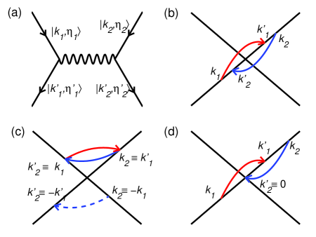
Figure 1: Scattering diagrams due to electron-electron interaction in which energy and momentum are conserved. (a) Feynmann diagram for the elastic e-e scattering. (b) Intra-intra-branch scattering. (c) Inter-inter-branch scattering ; (d) Intra-inter-branch scattering

Because intra-intra branch scattering is more efficient than inter-intra or inter-inter branch scattering, carrier populations in different branches behave as independent Fermi gases with specific temperatures. In the presence of an electric field $F$ an imbalance arises between carrier populations in different branches (different quasi-Fermi level $\mu_{\eta}$) with a nonzero current flow. Consequently the distribution functions in each (thermalized) branch reads:

$$f_{\eta}(E)=\frac{1}{\exp[(E-\mu_{\eta})/k_{B}T_{\eta}]+1}$$ (5)

where $T_{\eta}=T_{\eta}(z)$ is the local electronic temperature of the branch $\eta$. As the quasi-Fermi levels are far away from the band edges, and because the thermal broadening is much smaller than the band width, the carrier densities are independent of the respective temperatures due to the constant density of states. Since all the carriers share the same group velocity, the current is proportional to the quasi-Fermi level differenceKuroda et al. (2005), i.e.

$$I=ev_{F}(n_{+}-n_{-})=\frac{g_{c}e}{\pi\hbar}(\mu_{+}-\mu_{-})=g_{c}G_{0}\frac{(\mu_{+}-\mu_{-})}{e}$$ (6)

where $G_{0}=e^{2}/(\pi\hbar)$ is the quantum conductance. The factor $g_{c}$ accounts for the band degeneracy (spin degeneracy has already been considered). In Eq. 6 the current can be interpreted as the superposition of the electron current ($I_{+}$) and hole current ($I_{-}$):

$$I_{\pm}=\pm\frac{g_{c}e}{\pi\hbar}(\mu_{\pm}-\mu)=\frac{I}{2}$$ (7)

where $\mu\equiv(\mu_{+}-\mu_{-})/2$ is the effective Fermi level of the system. Similarly the internal energy flow per unit length for each branch with respect to the effective Fermi level is:

$$U_{\pm}=\pm\frac{g_{c}}{\pi\hbar}\int_{-\infty}^{\infty}(E-\mu_{\pm})\left[f_{\pm}(E)-\Theta(-E+\mu)\right]dE=\pm\frac{g_{c}}{\pi\hbar}\left[\frac{\pi^{2}(k_{B}T_{\pm})^{2}}{6}+\frac{(\mu_{+}-\mu_{-})^{2}}{8}\right],$$ (8)

where $\Theta(x)$ is the Heaviside step functioninf .

In the high (room) temperature semi-classical regime, the distribution function in each branch follows the stationary Boltzmann transport equation (BTE) which after making use of Eq. 2 reads:

$$\pm v_{F}\left[\,\partial_{z}f_{\pm}(E)+eF\partial_{E}f_{\pm}(E)\right]=\partial_{t}f_{\pm}\Big{\arrowvert}_{coll}.$$ (9)

Here $F$ and $\partial_{t}f_{\pm}\big{|}_{coll}$ are the electric field and the collision integral accounting for carrier scattering, respectively. We solve this equation using the method of moments, i.e. we multiply the BTE by $(E-\mu)^{m}$, where $m$ is the moment index, and integrate over energy, for which we obtain:

$$-e\left(F-\frac{1}{e}\partial_{z}\mu_{\pm}\right)=\pm\frac{2\pi\hbar}{g_{c}}\mathcal{F}_{0,\pm}^{coll}$$ (10)

and

$$\pm\partial_{z}U_{\pm}\mp\frac{I}{2}\left(F-\frac{1}{e}\partial_{z}\mu_{\eta}\right)=\mathcal{F}_{1,\pm}^{coll}$$ (11)

for the zeroth and first moment equations, respectively. $\mathcal{F}_{m,\eta}^{coll}\equiv\frac{g_{c}}{2\pi\hbar v_{F}}\int_{-\infty}^{\infty}(E-\mu)^{m}\partial_{t}f_{\eta}\big{|}_{coll}dE$ is the generalized $m$th moment of the collision integral for each branch. The left-hand side of Eq. 10 is the measured effective field ($F^{\prime}\equiv F-\partial_{z}\mu_{\pm}/e$) Ziman (1972), and we note that in general the expressions for $\mathcal{F}_{m,\eta}$ depend on both the local temperatures and current level (or difference between quasi-Fermi levels). This dependence couples the equations describing the heat flow (Eq. 11) for each carrier population. We solve both equations for the field and the temperatures profiles by using the current level as a parameter.

In the case of 1D metals, the main scattering process (other than e-e interaction) is scattering with phonons. We compute the collision integral for this mechanism as:

$$\frac{\partial f_{\eta}}{\partial t}\Big{\arrowvert}_{coll}=\sum_{q,\eta^{\prime}}\left\{R_{em}(q)\left[f_{\eta^{\prime}}(\epsilon_{+})\left(1-f_{\eta}(E)\right)-f_{\eta}(E)\left(1-f_{\eta^{\prime}}(\epsilon_{-})\right)\right]\right.$$

$$\left.R_{ab}(q)\left[f_{\eta^{\prime}}(\epsilon_{-})(1-f_{\eta}(E)-f_{\eta}(E)(1-f_{\eta^{\prime}}(\epsilon_{+})\right]\right\}$$ (12)

where $\epsilon_{\pm}=E\pm\hbar\omega_{q}$ and $q$ labels the phonon wave-vector. The prefactor $R_{em}$ ($R_{ab}$) is the phonon emission (absorption) rate. Here we focus on acoustic phonon scattering ($\omega_{q}=v_{s}|q|$), which we assume to be elastic (i.e. $v_{s}/v_{F}\ll 1$), and for which only the longitudinal modes contribute to the integral. Since phonon energies are much smaller than the lattice temperature $T_{L}$ ($\hbar\omega_{q}\ll k_{B}T_{L}$) and using the deformation potential approximation, we set $R_{em}=R_{ab}\propto T_{L}$ Hess (1999). We then define the mean free path $\lambda_{ac}\equiv v_{F}/R_{em}$.

By subtracting and adding the 0th moments of the BTE (Eq. 10) for the two carrier branches, we obtain:

$$\partial_{z}(\mu_{+}-\mu_{-})=0$$ (13)

and

$$I=g_{c}G_{0}\lambda_{ac}F^{\prime}$$ (14)

respectively. Eq. 13 expresses the local current conservation in the system ($I\propto\mu_{+}-\mu_{-}$). Eq. 14 is nothing but Ohm’s law for which the linear conductivity is inversely proportional to the lattice temperature ($\lambda_{ac}\propto T_{L}^{-1}$) but independent of the carrier temperatures $T_{\pm}$.

Using Eq. 7 we define the branch electrical conductivity as $\sigma_{\eta}\equiv g_{c}G_{0}\lambda_{ac}/2$. We emphasize that owing to the electron-hole symmetry Eq. 14 does not depend on the thermal gradient. Therefore, the thermoelectric power (TEP) in 1D (Dirac) conductors vanishes, which is in agreement with recent experiments on metallic carbon nanotubes that exhibit much smaller TEP than that of semiconducting carbon nanotubes Small et al. (2003).

In the presence of acoustic phonon scattering the 1st moment equation (Eq. 11) for each branch reads:

$$\partial_{z}U_{\pm}=\frac{IF^{\prime}}{2}\mp\frac{1}{\lambda_{ac}}\left(U_{+}+U_{-}\right)$$ (15)

Using Eqs. 8 and 13, the LHS of Eq. 15 is proportional to $\partial_{z}T_{\pm}$. This variation in the carrier temperature profiles is attributed to the Joule heating (first term on the RHS) and the inter-branch carrier scattering due to the carriers thermal imbalance (second term).

Combining Eq. 15 for the different branches we establish the heat flow conservation:

$$\partial_{z}(U_{+}+U_{-})=IF^{\prime}$$ (16)

which shows that all the heat is transported by the electrons and results in an inhomogeneous temperature profile. This is consistent with our approximation of elastic phonon scattering for which no energy gained by the carriers from the external field is transferred to the lattice (i.e. the lattice temperature remains constant). The energy production/dissipation in the system couples the two carrier temperatures $T_{\pm}$ (Eq. 15). Furthermore, Eq. 16 validates the assumption of the two temperature model for the electronic population in each branch. Indeed, if $T_{+}(z)=T_{-}(z)$ the LHS of Eq. 16 vanishes, which is inconsistent with a non-zero current.

Substituting Eq. 8 into Eq. 16 we obtain for the heat flow:

$$\mp\frac{\lambda_{ac}g_{c}\pi k_{B}^{2}T_{\pm}}{3\hbar}\partial_{z}T_{\pm}=U_{+}+U_{-}\mp\frac{\lambda_{ac}IF^{\prime}}{2}$$ (17)

for which the pre-factor in the temperature gradient is the carrier thermal conductivity:

$$\kappa_{\eta}=\frac{\lambda_{ac}g_{c}\pi k_{B}^{2}T_{\eta}}{3\hbar}=\lambda_{ac}g_{c}G_{th}$$ (18)

where $G_{th}$ is the quantized thermal conductance Rego and Kirczenow (1998). The ratio between thermal and electrical conductivity for each branch:

$$\frac{\kappa_{\eta}}{\sigma_{\eta}T_{\eta}}=\frac{2\pi^{2}k_{B}^{2}}{3e^{2}}$$ (19)

obeys Wiedemann-Franz law with their specific carrier temperature and a proportionality factor that is twice the Lorenz number (for 2 and 3 dimensions) Ziman (1972).

In the case of isothermal lattices, $\lambda_{ac}$ and $F$ are constant, and by assuming ideal contacts (i.e. completely absorbing and thermalizing) $T_{\pm}(\mp L/2)=T_{0}$ , the solution of Eq. 15 is:

$$T_{\pm}(z)=T_{0}\sqrt{1+\frac{3}{\pi^{2}}\left[1+\frac{1\mp 2z/L}{2\lambda_{ac}/L}\right]\frac{1\pm 2z/L}{2\lambda_{ac}/L}\left(\frac{I}{I_{T_{0}}}\right)^{2}}$$ (20)

for which $I_{T_{0}}\equiv(g_{c}ek_{B}T_{0})/(\pi\hbar)$ is the current associated to the lattice temperature. The temperature of the carriers with positive (negative) Fermi velocity has a maximum at $z=\lambda_{ac}$ ($z=-\lambda_{ac}$). In the quasi-ballistic limit, $\lambda_{ac}\gg L$, the carrier temperature profiles $T_{\pm}^{QB}(z)$ have a linear $z$-dependence:

$$\frac{T_{\pm}^{QB}(z)}{T_{0}}=1+\frac{3L}{4\pi^{2}\lambda_{ac}}\left(\frac{I}{I_{T_{0}}}\right)^{2}\left(1\pm\frac{2z}{L}\right)$$ (21)

In this regime, the temperature difference $T_{\pm}-T_{0}$ is small even for $I\sim I_{T_{0}}$ because of the ratio $L/\lambda_{ac}\ll 1$. In the diffusive regime ($\lambda_{ac}\ll L$), the carrier temperature profiles have a parabolic shape and the maximum temperature difference is of the same order as $T_{0}$ even for small current levels. In Fig. 2 we display the temperature and heat flow profiles corresponding to carrier populations with positive Fermi velocity ($T_{+}(z,I)$ and $U_{+}(z,I)$) for ratios $L/\lambda_{ac}=0.05$, 1 and 4, respectively. The electron-hole symmetry in this case is expressed by the fact that $T_{+}(z)=T_{-}(-z)$ and $U_{+}(z)=-U_{-}(-z)$.

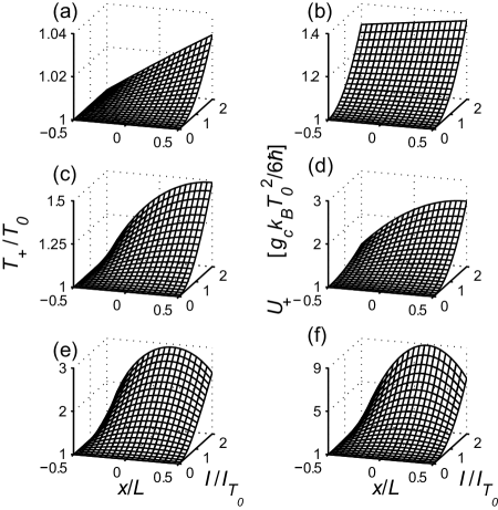
Figure 2: Temperature profiles ($T_{+}$) and heat flow $U_{+}$ for carriers with positive Fermi velocity as a function of the current for: $\lambda_{ac}=20L$ (a,b), $\lambda_{ac}=L$ (c,d), and $\lambda_{ac}=0.25L$ (e,f).

If a lattice temperature gradient exists along the conductor $T_{L}(z)=T_{0}-\Delta T\,z/L)$, the carrier temperature profiles are:

$$T_{\pm}(z)=\sqrt{\left(T_{0}\pm\frac{\Delta T}{2}\right)^{2}+\frac{L}{L+\lambda_{0}}\left[\left(T_{0}-\Delta T\frac{z}{L}\right)^{2}-\left(T_{0}\pm\frac{\Delta T}{2}\right)^{2}\right]}$$ (22)

for which we have assumed $\lambda_{ac}(z)T_{L}(z)=\lambda_{0}T_{0}$ (Eq. 14) and the symmetric boundary conditions $T_{L}(-L/2)=T_{+}(-L/2)$ and $T_{L}(L/2)=T_{-}(L/2)$. For $\Delta T\ll T_{0}$, Eq. 22 becomes:

$$T_{\pm}(z)=T_{0}-\frac{\Delta T}{2}\frac{(2z\mp\lambda_{0})}{(L+\lambda_{0})}$$ (23)

and the carrier temperature difference reads,

$$T_{+}(z)-T_{-}(z)=\Delta T\frac{\lambda_{ac}}{L+\lambda_{ac}}.$$ (24)

In the case of ballistic transport ($\lambda_{ac}/{L}\gg 1$) the temperature difference remains $T_{+}-T_{-}=\Delta T$ along the conductor, while for diffusive transport ($\lambda_{ac}/{L}\ll 1$), the temperature difference between branches is negligible.

It is important to emphasize that Eqs. 10 and 11 are valid both in low and high field regimes. However, here we only consider elastic scattering and thereby the results are valid in the linear regime (i.e. low current levels and $\hbar\omega_{q}\ll k_{B}T_{L}$). At high current levels, other scattering processes (e.g. optical phonon scattering) have to be included in the collision integrals.

In conclusion because of the effective intrabranch carrier thermalization in the high temperature regime electron populations in the different branches of 1D Dirac conductors behave as independent Fermi gases (with their respective temperatures) out of thermal equilibrium as a consequence of the electro-thermal flow. In the presence of acoustic phonon scattering, the carrier population in each energy branch follows the Wiedemann-Franz law characterized by twice the Lorenz number. The TEP coefficient in 1D conductors vanishes as a result of the electron-hole symmetry.

References

- Hu et al. (1999) J. Hu, T. Odom, and C. Lieber, Accounts of Chemical Research 32, 435 (1999), ISSN 0001-4842, URL http://pubs3.acs.org/acs/journals/doilookup?in_doi=10.1021/ar%9700365.
- Sólyom (1979) J. Sólyom, Advances in Physics 28, p201 (1979), ISSN 00018732.
- Voit (1995) J. Voit, Reports on Progress in Physics 58, 977 (1995), URL http://stacks.iop.org/0034-4885/58/977.
- Yacoby et al. (1996) A. Yacoby, H. L. Stormer, N. S. Wingreen, L. N. Pfeiffer, K. W. Baldwin, and K. W. West, Phys. Rev. Lett. 77, 4612 (1996).
- Bockrath et al. (1999) M. Bockrath, D. H. Cobden, J. Lu, A. G. Rinzler, R. E. Smalley, L. Balents, and P. L. McEuen, Nature 397, 598 (1999), URL http://dx.doi.org/10.1038/17569.
- Zaitsev-Zotov et al. (2000) S. V. Zaitsev-Zotov, Y. A. Kumzerov, Y. A. Firsov, and P. Monceau, Journal of Physics: Condensed Matter 12, L303 (2000), URL http://stacks.iop.org/0953-8984/12/L303.
- Deshpande and Bockrath (2007) V. Deshpande and M. Bockrath, Nature Physics 32, 314 (2007).
- Park et al. (2004) J.-Y. Park, S. Rosenblatt, Y. Yaish, V. Sazonova, H. Ustunel, S. Braig, T. Arias, P. Brouwer, and P. McEuen, Nano Lett. 4, 517 (2004), URL http://dx.doi.org/10.1021/nl035258c.
- Kuroda et al. (2005) M. A. Kuroda, A. Cangellaris, and J.-P. Leburton, Phys. Rev. Lett. 95, 266803 (pages 4) (2005), URL http://link.aps.org/abstract/PRL/v95/e266803.
- Lazzeri and Mauri (2006) M. Lazzeri and F. Mauri, Phys. Rev. B 73, 165419 (pages 6) (2006), URL http://link.aps.org/abstract/PRB/v73/e165419.
- Javey et al. (2004) A. Javey, J. Guo, M. Paulsson, Q. Wang, D. Mann, M. Lundstrom, and H. Dai, Phys. Rev. Lett. 92, 106804 (pages 4) (2004), URL http://link.aps.org/abstract/PRL/v92/e106804.
- Leburton (1992) J. P. Leburton, Phys. Rev. B 45, 11022 (1992).
- (13) The Heaviside function is introduced to eliminate the artificial divergence arising from the extension of the bottom of the conduction bands to infinity in the integration.
- Ziman (1972) J. M. Ziman, Principles of the Theory of Solids, 2nd ed. (Cambridge University, Cambridge, England, 1972).
- Hess (1999) K. Hess, Advanced Theory of Semicondutor Devices (IEEE Press, New York, 1999).
- Small et al. (2003) J. P. Small, K. M. Perez, and P. Kim, Phys. Rev. Lett. 91, 256801 (2003).
- Rego and Kirczenow (1998) L. G. C. Rego and G. Kirczenow, Phys. Rev. Lett. 81, 232 (1998).