Optimal potentials for temperature ratchets

Abstract

In a spatially periodic temperature profile, directed transport of an overdamped Brownian particle can be induced along a periodic potential. With a load force applied to the particle, this setup can perform as a heat engine. For a given load, the optimal potential maximizes the current and thus the power output of the heat engine. We calculate the optimal potential for different temperature profiles and show that in the limit of a periodic piecewise constant temperature profile alternating between two temperatures, the optimal potential leads to a divergent current. This divergence, being an effect of both the overdamped limit and the infinite temperature gradient at the interface, would be cut off in any real experiment.

I Introduction

Noise induced transport occurs in a broad variety of systems both in physics and biology Reimann (2002). In a microscopic system embedded in a thermal environment, directed transport generally requires two ingredients: (i) External sources driving the system out of equilibrium and (ii) broken spatial symmetry Reimann (2002). The main idea is to impede the thermal motion in one direction in order to obtain a net current in the other direction Astumian and Bier (1994). This mechanism is called the “ratchet effect”. Applications range from particle sorting Faucheux and Libchaber (1995); Rousselet et al. (1994) to modeling molecular motors Cordova et al. (1992); Astumian and Bier (1994); Jülicher et al. (1997); Astumian and Hänggi (2002). Most studies on ratchet motors focus on a given potential landscape and a given driving scheme. For practical purposes, however, optimization of the driving mechanism with respect to a maximal current is an important issue.

For discrete analogues of ratchet motors, where the potential landscape is characterized by only a few parameters, such an optimization has been performed in models for microscopic heat engines Tu (2008) and molecular motors Schmiedl and Seifert (2008a). Paradoxical Parrondo games Parrondo et al. (2000) which can be interpreted as discrete analogues of Brownian ratchets Amengual et al. (2004), have also been optimized recently Dinis (2008).

For continuous motors, where optimization requires variational calculus, there exist only few results. The optimization of driving schemes has been studied for time-dependently driven ratchet motors Tarlie and Astumian (1998); Lade (2008) and for a Brownian heat engine cycling between two heat reservoirs Schmiedl and Seifert (2008b). Potential landscapes have been optimized for the transport across membrane channels Bezrukov et al. (2007). Maximizing the current of flashing ratchets by using a feedback control strategy has been proposed recently Cao et al. (2004); Craig et al. (2008).

In this paper, we focus on a continuous thermal ratchet where transport along a spatially varying time-independent potential is driven by a periodic spatial temperature profile Feynman et al. (1966); Büttiker (1987); Landauer (1988); Blanter and Büttiker (1998). The recent generation of temperature gradients on small length scales Duhr and Braun (2006, 2007); Weinert et al. (2008) may render such molecular heat engines experimentally realizable. Cargoes driven by thermal gradients on a subnanometer scale have already been observed Barreiro et al. (2008).

Thermodynamic efficiencies of such ratchet heat engines have been calculated in Refs. Jarzynski and Mazonka (1999); Matsu and Sasa (2000); Benjamin and Kawai (2008). It has been argued that heat engines should generally be characterized by their performance at maximum power output Curzon and Ahlborn (1975); Van den Broeck (2005). Recent studies on ratchet heat engines have varied the load force for a constant potential in order to maximize the power output Asfaw and Bekele (2004); Gomez-Marin and Sancho (2006). We take a complementary approach and optimize the potential for a given load. The maximization of power output and particle current then is equivalent.

So far, this task has been tackled numerically only for a one-parameter class of potentials for a given temperature Asfaw (2008). To the best of our knowledge, there exists no systematic study on the optimal potential for such a thermal ratchet. Using variational calculus we determine the optimal potential which maximizes the current for a given temperature analytically up to a numerical root search. For a dichotomous temperature profile with infinitely steep gradients as used in most previous studies Asfaw and Bekele (2004); Gomez-Marin and Sancho (2006); Benjamin and Kawai (2008), the maximal current diverges. This unphysical behaviour is an effect of the idealized assumptions of both an infinite temperature gradient at the interface and the overdamped dynamics. In any realistic system, temperature gradients will be finite which is sufficient to cut off the formal divergence.

II The temperature ratchet and its current

We consider a Brownian particle of mass $m$ moving in a periodic potential $V(x)$ with $V(x+L)=V(x)$ in a viscous fluid with friction coefficient $\gamma$. A constant load $f$ is attached to the particle. The surrounding temperature is modeled by $T(x)$ which has the same periodicity $L$ as the potential. A special case is a piecewise constant temperature with a hot and a cold area, see Fig. 1. For a properly chosen potential the particle moves against the load on average. The thermal fluctuations in the hot area can push the particle against the load over the barrier of the potential. As soon as the particle is in the cold area the probability of getting pushed back is smaller because of the weaker thermal fluctuations. In this way the particle drags the load and produces work effectively acting as a heat engine that works between two heat baths. Such a mechanism is not limited to piecewise constant temperatures.

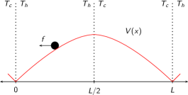
Figure 1: A temperature ratchet: a particle with a load $f$ moving in a potential $V(x)$ in two piecewise constant temperature regions $T_{h}$ and $T_{c}$.

The time evolution of the position of the particle $x(t)$ is governed by the Langevin equation

$$m\ddot{x}=-\gamma\dot{x}-V^{\prime}(x)+f+g(x)\xi(t),$$ (1)

where time derivatives are denoted by dots and space derivatives by primes. The stochastic term $g(x)\xi(t)$ models the thermal noise from the environment. Its strength

$$g(x)\equiv\sqrt{{k_{B}T(x)}{\gamma}}$$ (2)

depends on the temperature profile $T(x)$ resulting in multiplicative noise.

In the following we want to make two assumptions: the friction dominates the inertia and the noise is uncorrelated Gaussian. When dealing with multiplicative noise, these two limiting procedures do not commute Sancho et al. (1982); Kupferman et al. (2004). The order of the limiting procedures determines the stochastic interpretation of the term $g(x)\xi(t)$. If we first assume Gaussian white noise

$$\left\langle\xi(t)\xi(t^{\prime})\right\rangle=2\delta(t-t^{\prime}),$$ (3)

and then go to the overdamped equation

$$\gamma\dot{x}=-V^{\prime}(x)+f+g(x)\xi(t)$$ (4)

we end up with a corresponding Fokker-Planck equation

$$\partial_{t}p(x,t) =-\partial_{x}\left[\frac{1}{\gamma}\left(-V^{\prime}(x)+f\right)-\frac{1}{\gamma^{2}}\partial_{x}g^{2}(x)\right]p(x,t)$$ (5)

$$=-\partial_{x}j(x,t)$$

in Ito’s sense where $j(x,t)$ is the current and $p(x,t)$ the probability distribution.

If we first take the overdamped limit and afterwards assume Gaussian white noise, we end up with a Fokker-Planck equation in Stratonovich’s sense. Both equations differ in a drift term which can be absorbed in an effective potential. Thus, the optimal current does not depend on the interpretation. The optimal potential is merely shifted by the drift term. In the following we use the Fokker-Planck equation in Ito’s sense.

We next introduce dimensionless units. We express energies in units of $k_{B}T_{0}$ where

$$T_{0}\equiv\frac{1}{L}\int_{0}^{L}T(x)\>dx.$$ (6)

By introducing a scaled length $\hat{x}\equiv x/L$ and a scaled time $\hat{t}\equiv t/t_{0}$ with $t_{0}\equiv L^{2}\gamma/k_{B}T_{0}$, we rewrite the Fokker-Planck equation and identify the dimensionless quantities

$$\hat{T}(\hat{x}) \equiv\frac{T(x)}{T_{0}}, \hat{V}(\hat{x}) \equiv\frac{V(x)}{k_{B}T_{0}}, \hat{f} \equiv\frac{fL}{k_{B}T_{0}},$$

$$\hat{\jmath}(\hat{x},\hat{t}) \equiv\frac{j(x,t)L^{2}\gamma}{k_{B}T_{0}}, \hat{p}(\hat{x},\hat{t}) \equiv Lp(x,t).$$ (7)

For ease of notation we drop the hats in the following. The dimensionless potential $V(x)$ and the dimensionless temperature profile $T(x)$ are periodic, $V(x+1)=V(x)$, $T(x+1)=T(x)$. In the steady state, the current $j$ is a constant and the Fokker-Planck equation reduces to

$$j=[-V^{\prime}(x)+f-T^{\prime}(x)]p(x)-T(x)\partial_{x}p(x).$$ (8)

For a periodic temperature we solve this equation under the condition of a periodic $p(x)$. Without loss of generality, we chose $V(0)=0$ which results in

$$p(x)=\frac{je^{\phi(x)}}{T(x)}\left(\frac{1}{1-e^{-\phi(1)}}\int_{0}^{1}e^{-\phi(x^{\prime})}\>dx^{\prime}-\int_{0}^{x}e^{-\phi(x^{\prime})}\>dx^{\prime}\right)$$ (9)

with

$$\phi(x)\equiv\int_{0}^{x}\frac{-V^{\prime}(x^{\prime})+f}{T(x^{\prime})}\>dx^{\prime}.$$ (10)

Using the normalization $\int_{0}^{1}p(x)dx=1$, we obtain the inverse current

$$j^{-1}=\frac{1}{1-e^{-\phi(1)}}\int_{0}^{1}e^{-\phi(x^{\prime})}\>dx^{\prime}\int_{0}^{1}\frac{e^{\phi(x)}}{T(x)}\>dx\\ -\int_{0}^{1}\left(\int_{0}^{x}e^{-\phi(x^{\prime})}\>dx^{\prime}\right)\frac{e^{\phi(x)}}{T(x)}\>dx$$ (11)

which has been derived previously in Refs. Büttiker (1987); Asfaw and Bekele (2004).

III Optimizing the current

The inverse current [Eq. (11)] depends on the shape of the potential $V(x)$. Instead of optimizing the current directly with respect to the potential we introduce

$$B(x)\equiv\int_{0}^{x}e^{-\phi(x^{\prime})}\>dx^{\prime}$$ (12)

and rewrite the inverse current in a more elegant way as a functional of $B(x)$

$$j^{-1}[B,B^{\prime}]=\int_{0}^{1}\frac{\alpha-B(x)}{T(x)B^{\prime}(x)}\>dx$$ (13)

with

$$\alpha\equiv\frac{B(1)}{1-B^{\prime}(1)}.$$ (14)

For the minimization of the functional (13), the function space is constrained by the periodicity of the potential which imposes a constraint on $B(x)$. With the boundary condition $V(1)=V(0)=0$ we obtain from Eq. (10) the non-local constraint

$$\int_{0}^{1}\phi^{\prime}T\>dx=f$$ (15)

which by using Eq. (12) can be transformed into the isoperimetric constraint

$$\int_{0}^{1}T^{\prime}\ln B^{\prime}\>dx=f+T\ln B^{\prime}\Big{|}_{0}^{1}.$$ (16)

In order to minimize the inverse current [Eq. (13)] under the constraint [Eq. (16)] we introduce the effective Lagrangian

$$\mathcal{L}[B(x),B^{\prime}(x),x]\equiv\frac{\alpha-B(x)}{T(x)B^{\prime}(x)}+\lambda T^{\prime}(x)\ln B^{\prime}(x)$$ (17)

with a Lagrange multiplier $\lambda$.

For a unique solution to the corresponding Euler-Langrange equation we have to impose two boundary conditions. The first one, $B(0)=0$, arises naturally from the definition of $B(x)$ in Eq. (12). One is tempted to use the condition $B^{\prime}(0)=1$ as the second one, but this is not appropriate. In principle, we have to allow the derivative to jump at the boundaries because such jumps do not contribute to the integral of the Lagrangian. In this way the boundary condition fixes the value $B^{\prime}(0)=1$, but the value of $\lim_{\epsilon\to 0}B^{\prime}(0+|\epsilon|)$, which is the relevant boundary condition for the solution of the Euler-Langrange equation, in fact, remains a free parameter. This feature has been discussed in detail for similar optimization problems Schmiedl and Seifert (2007); Gomez-Marin et al. (2008).

For the optimization we proceed in two steps. First we minimize the integral of the Lagrangian $\int_{0}^{1}\mathcal{L}\>dx$ and then we adjust the remaining parameters to obtain the maximum current. The corresponding Euler-Langrange equation is given by

$$2B^{\prime 2}T+(\alpha-B)(T^{\prime}B^{\prime}+2TB^{\prime\prime})+\lambda T^{2}B^{\prime}(T^{\prime\prime}B^{\prime}-T^{\prime}B^{\prime\prime})=0$$ (18)

with the boundary condition $B(0)=0$. Changing variables $B(x)=-\alpha\exp[I(x)]+\alpha$ leads to a second order differential equation for $I(x)$ which is integrable. The solution

$$I_{\pm}(x)\equiv\int_{0}^{x}\frac{2\>dx^{\prime}}{-\lambda TT^{\prime}\pm\sqrt{4T(c+\lambda T)+\lambda^{2}T^{2}T^{\prime 2}}}$$ (19)

still depends on the Lagrange multiplier $\lambda$ and the new constant $c$. The solution of the Euler-Lagrange equation

$$B(x)=-\alpha\exp[I_{\pm}(x)]+\alpha$$ (20)

leads to the optimal inverse current

$$j^{-1}(\lambda,c) =-\int_{0}^{1}\frac{dx}{T(x)I^{\prime}_{-}(x)}$$

$$=\frac{1}{2}\int_{0}^{1}\left[\sqrt{4\left(\frac{c}{T}+\lambda\right)+\lambda^{2}T^{\prime 2}}\;\right]\>dx$$ (21)

which depends on the two parameters $\lambda$ and $c$ but is independent of $\alpha$. Note that in order to obtain a positive current, we chose the minus sign of the square root in Eq. (19).

In the next step, we optimize the inverse current [Eq. (III)] by adjusting the free parameters $\lambda$ and $c$. These parameters are not independent but related by the constraint [Eq. (16)]

$$n(\lambda,c)\equiv T\ln|I_{-}^{\prime}|\Big{|}_{0}^{1}+f-\int_{0}^{1}T^{\prime}\ln|I_{-}^{\prime}|\;dx+\int_{0}^{1}I_{-}^{\prime}T\;dx=0.$$ (22)

In the appendix, we show that in general the optimization problem has a solution for $c=0$. Hence, for a given temperature profile the remaining parameter $\lambda$ can be determined by the constraint [Eq. (22)].

From Eqs. (10, 12, 20) we derive the optimal potential

$$V(x)=T\ln|I_{-}^{\prime}|\Big{|}_{0}^{x}+fx-\int_{0}^{x}T^{\prime}\ln|I_{-}^{\prime}|\;dx^{\prime}+\int_{0}^{x}I_{-}^{\prime}T\;dx^{\prime}$$ (23)

which becomes the basis for the following case studies.

IV Case study I: Sinusoidal temperature profile

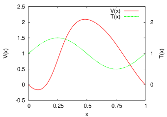
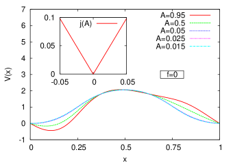
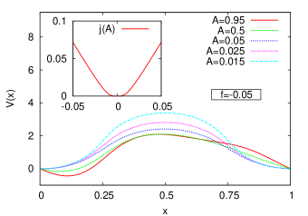
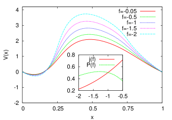
Figure 2: (a) Optimal potential $V(x)$ and $T(x)=\frac{1}{2}\sin(2\pi x)+1$ for load $f=-0.05$. (b) Optimal potentials $V(x)$ for $T(x)=A\sin(2\pi x)+1$ with different amplitudes $A$ and load $f=0$. Inset: Optimal current $j$ versus $A$. (c) Optimal potentials $V(x)$ for $T(x)=A\sin(2\pi x)+1$ with different amplitudes $A$ and load $f=-0.05$. Inset: Optimal current $j$ versus $A$. (d) Optimal potentials $V(x)$ for $T(x)=\frac{1}{2}\sin(2\pi x)+1$ and for different loads $f$. Inset: Optimal current $j(f)$ and power $P(f)$ as a function of the force. The power exhibits a maximum $P_{\rm{opt}}\simeq 0.52$ at $f_{\rm{opt}}\simeq-1.27$.

In this section we will discuss a sinusoidal temperature profile

$$T(x)=A\sin(2\pi x)+1$$ (24)

with the amplitude $0<A<1$. The external force $f$ is a second parameter. In the following we will study how the optimal potential and the current depend on these two parameters.

The height of the potential is the essential blocking mechanism in the ratchet. The thermal “kicks” from the environment move the particle over this barrier. We expect the largest slope of the optimal potential roughly at the hottest point because there the fluctuations are strong enough to push the particle against a large force. In the colder regions, the potential should decrease. The optimal potential as determined numerically using Eq. (23) indeed fulfills these expectations, see Fig. 2.

IV.1 Optimal potential for different amplitudes of the temperature profile

The optimal potential for different amplitudes $A$ with zero external force $f=0$ is shown in Fig. 2. For amplitudes $A\rightarrow 1$, the temperature in the colder area $x>0.5$ goes to zero and the optimal potential becomes strongly asymmetric. In this low temperature area the thermal fluctuations are so weak that even a gently declining potential is sufficient to push the particle in one direction. The optimal current is proportional to the absolute value of the amplitude, see Fig. 2. This general scaling behavior is not limited to a sinusoidal temperature profile which can be understood as follows. With the periodicity $T^{\prime}(0)=T^{\prime}(1)$, the first term of the constraint [Eq. (22)] vanishes. With $c=0$ and $f=0$, Eq. (22) and Eq. (III) become

$$n(\lambda)=\int_{0}^{1}T^{\prime}\ln\left|\lambda T^{\prime}+\sqrt{4\lambda+\lambda^{2}T^{\prime 2}}\right|\\ -\frac{1}{2\lambda}\sqrt{4\lambda+\lambda^{2}T^{\prime 2}}\>dx=0$$ (25)

and

$$j^{-1}(\lambda)=\frac{1}{2}\int_{0}^{1}\sqrt{4\lambda+\lambda^{2}T^{\prime 2}}\>dx.$$ (26)

The derivative of the temperature scales like $T^{\prime}(x)\propto A$. Choosing $\lambda\propto A^{-2}$, the constraint [Eq. (25)] is independent of $A$. The current [Eq. (26)] then is a linear function of $A$.

Now we consider the system with a finite external force, $f=-0.05$. For temperature amplitudes $A\rightarrow 1$, effectively corresponding to a large temperature difference, the external force can be neglected and the optimal potential looks like in the case without an external force, see Fig. 2. For small $A$, the ratchet effect induced by the temperature difference is not strong enough against the external force. In this regime, the optimal potential has to prevent the particle from being dragged in the direction of the external force. This is achieved by blocking the particle with a larger barrier, see Fig. 2.

IV.2 Optimal potential for different external forces

For stronger external forces, the potential has to compensate this dragging mechanism with a larger barrier in order to obtain a current in the direction opposite to the force. Thus, we expect larger potentials and smaller currents for stronger external forces which is confirmed by our calculations, see Fig. 2.

We next calculate the dimensionless power output of the heat engine which is given by

$$P\equiv-fj.$$ (27)

The power output as a function of the force $f$ is shown in the inset in Fig. 2. It exhibits a maximum at intermediate forces where the heat engine thus works in a maximum power regime.

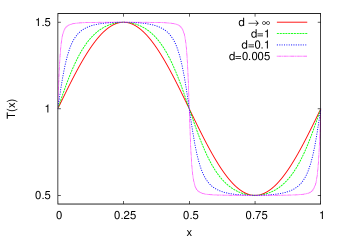
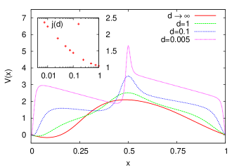
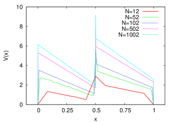
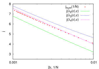
Figure 3: (a) Continuous approximation $T(x)$ [Eq. (29)] to a piecewise constant temperature for different parameters $d$. In the limit $d\to\infty$, $T(x)$ approaches the sinusoidal profile $T(x)=\frac{1}{2}\sin(2\pi x)+1$. (b) Optimal potentials $V(x)$ for $T(x)$ from Fig. 3 with external force $f=-0.05$. Inset: current $j$ versus parameter $d$. (c) Optimal potentials obtained from the numerical minimization on a discrete lattice for a piecewise constant temperature profile $T(x)$ [ Eq. (28)] with $\Delta T=1/2$ and with an external force $f=-0.05$ for different discretization $N$. (d) For an external force $f=-0.05$, optimal current $j_{\rm{num}}$ as obtained from the numerics with discretization $2\epsilon=1/N$ compared to the perturbative calculation developed in the appendix.

V Case study II: Piecewise constant temperature

We now consider a piecewise constant temperature

$$T(x)=1+\Delta T-2\Delta T\Theta(x-1/2)$$ (28)

with a hot and a cold area with temperatures $T_{h}\equiv 1+\Delta T$ and $T_{c}\equiv 1-\Delta T$, respectively, where $0<\Delta T<1$. We then face discontinuities in the Fokker-Planck equation. In this section, we first analyze a continuous approximation to the piecewise constant temperature. The optimal potential then has an complex shape with peaks. We compare these results with a numerical solution for the optimal potential.

The continuous temperature profile

$$T(x)=\frac{\sqrt{1+d}\sin(2\pi x)}{2\sqrt{\sin^{2}(2\pi x)+d}}+1$$ (29)

interpolates between the extreme values $d\to 0$ which corresponds to the piecewise constant temperature [Eq. (28)] with $\Delta T=1/2$ and $d\to\infty$ where the profile becomes sinusoidal [Eq. 24] with $A=1/2$, see Fig. 3.

The optimal potential for different values of the parameter $d$ is shown in Fig. 3. For $d\ll 1$, two peaks emerge in the optimal potential at the positions of the temperature discontinuities. In between these two peaks, the potential decreases linearly. The current diverges for $d\to 0$, see inset of Fig. 3.

V.1 Numerical solution for a piecewise constant temperature

We next investigate this complex shape of the potential and the divergent current in more detail by solving the problem numerically on a discrete lattice. The goal is to minimize the inverse current [Eq. (11)] for the piecewise constant temperature [Eq. (28)]. The periodic boundary condition [Eq. (15)] for the potential transforms to the condition

$$\phi(1)=\phi(1/2)\left(\frac{2\Delta T}{\Delta T-1}\right)+\frac{f}{1-\Delta T}$$ (30)

considering that $\phi(0)=0$ by definition [Eq. (10)]. For a numerical solution we discretize $\phi(x)\rightarrow\phi(x_{i})\equiv\phi_{i}$ with $i=0,\dots,N$ and search for a global minimum of $j^{-1}(\phi_{i})$ in this $N+1$-dimensional space with a simplex algorithm proposed by Nelder and Mead Nelder and Mead (1965). The boundary values $\phi_{0}$ and $\phi_{N}$ are given according to Eqs. (10, 30) by

$$\phi_{0} =0,$$ (31)

$$\phi_{N} =\phi_{N/2}\left(\frac{2\Delta T}{\Delta T-1}\right)+\frac{f}{1-\Delta T}$$ (32)

and $\phi_{1},\dots,\phi_{N-1}$ are varied to yield a maximum current. Using Eq. (10), we then calculate the potential $V(x)$ from the optimal $\phi(x)$.

The numerical solution for the optimal potential depends on the discretization which determines how large the gradient of the temperature and the potential can be, see Fig. 3. For finer discretization, the optimal potential shows larger gradients. As a consequence, we find that the current $j_{\rm{num}}(N)$ diverges with increasing discretization $N\to\infty$, see Fig. 3. This is consistent with the developing divergence visible in Fig. 3.

V.2 Origin of the divergent current

Figure 4: Temperature profile on the lattice with gradients depending on $\epsilon$.

Due to the lattice discretization, the temperature profile can be considered to be linear with gradients with absolute value $1/(2\epsilon)$, see Fig. 4. We calculate the optimal inverse current [Eq. (III)] for such a temperature profile

$$j^{-1}(\lambda,\epsilon)=\sqrt{\lambda^{2}+16\lambda\epsilon^{2}}+\sqrt{\lambda}(1-4\epsilon).$$ (33)

The Lagrange multiplier $\lambda$ and the discretization parameter $\epsilon$ are related by the corresponding constraint [Eq. (22)]

$$\ln\left|1+\frac{\lambda}{8\epsilon^{2}}+\frac{1}{4\epsilon}\sqrt{\frac{\lambda^{2}}{4\epsilon^{2}}+4\lambda}\right|-\sqrt{1+\frac{16\epsilon^{2}}{\lambda}}+\frac{4\epsilon-1}{\sqrt{\lambda}}+f=0.$$ (34)

In the appendix, we show with a perturbation method that for $\epsilon\rightarrow 0$, the constraint [Eq. (34)] can be fulfilled if $\lambda\rightarrow 0$. For an approximated dependence $\lambda(\epsilon)$, we use an iterative method and obtain a sequence of functions

$$\lambda_{n+1}(\epsilon)=\frac{1}{(\ln|\lambda_{n}(\epsilon)|-2\ln|2\epsilon|-1+f)^{2}}$$ (35)

with $\lambda_{0}=1$. For the first members we calculate the current [Eq. (33)] as a function of $\epsilon$. These results are compared to the numerical current, where the discretization $1/N$ corresponds to $2\epsilon$, see Fig. 3. The divergent behavior of the current obtained from perturbation theory is in good agreement with the divergence from the numerics. The discrepancy is on one hand due to the numerical integration on the lattice in Eq. (11) and on the other hand due to the approximations implicit in the perturbation method.

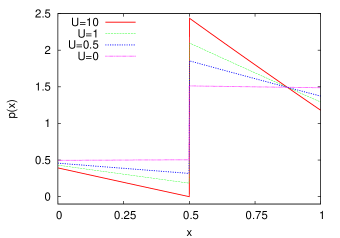
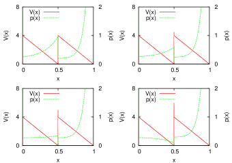
Figure 5: (a) Probability distributions for a rising peak with height $U$ in a piecewise constant temperature $T(x)$ [Eq. (28)] with $\Delta T=1/2$ and load $f=-0.05$. (b) Sawtooth potential with superimposed peak and its corresponding probability distribution in a piecewise constant temperature $T(x)$ [Eq. (28)] with $\Delta T=1/2$ and load $f=-0.05$ for different peak heights.

More insight into the origin of the divergent current can be gained from analyzing the probability distribution [Eq. (9)] which can be calculated from the Fokker-Planck equation for a model potential. Guided by the optimal potential obtained from the numerics, see Fig. 3, we consider a sawtooth potential with a superimposed finite peak at the temperature discontinuity at $x=0.5$. Note that we use this potential only as a case study aiming at a deeper understanding of the divergence of the current. The full optimal potential has a second peak at $x=0$ and both the height of the peaks and the linear slopes between the peaks diverge.

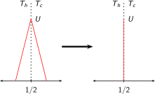
Figure 6: Peak as a limiting process. Each side is in one temperature region.

A finite peak potential is not a $\delta$-function, but can be considered as a result of a limiting process from a triangular shape, see Fig. 6. It is important that the peak arises at the discontinuity of the temperature profile, namely that the rising side of the peak is in one temperature area and the other side is in the other temperature area. Otherwise the peak would not contribute to the integrals in the current. Since the peak has infinitesimally small width, the forward rate is not decreased by a higher peak potential, contrary to a rising barrier with finite width. A finite peak in a constant temperature area would not contribute to integrals and thus would have no effect on mean first passage times. In contrast, for a dichotomous temperature profile and a finite peak at the interface, mean first passage times involving a crossing of the peak are affected by its height. The backward mean first passage time increases exponentially with the peak height. In contrast and somewhat counter-intuitively, the forward mean first passage time decreases with increasing peak height due to the strong suppression of peak recrossings from the cold side.

A finite peak with height $U$ superimposed on a flat potential causes a depletion of the particles on the high temperature side and an accumulation on the other side. With increasing peak height $U$, this behavior saturates, see Fig. 5. In a sawtooth potential, the particles accumulate in front of the barriers, see Fig. 5. If we combine both effects by superimposing a finite peak on a sawtooth potential, the depletion can compensate the accumulation, see Fig. 5.

The compensation of the accumulation is the main reason for the divergent current. For a sawtooth potential with large amplitude, the particles would accumulate in front of the barriers. The peaks counteract this effect and allow the particles to overcome the barriers. In between the peaks, the particles (on average) follow the steep potential with large mean velocity. For finer discretization, the peaks get larger and the potential in between steeper corresponding to a stronger force which increases the mean velocity and thus the current.

This behavior is only valid under the assumption of an overdamped dynamics where the particle instantaneously adjusts its velocity according to the Langevin equation (4). In the underdamped case, the particle needs a certain distance to reach the velocity corresponding to the local force. The overdamped limit is a good approximation as long as the relaxation time of the momentum $\tau_{R}\equiv m/\gamma$ is small compared to the (mean) time $\tau_{c}$ it takes for the particle to cross a region with basically constant force. Considering the potential above with discretization $\epsilon$, both the peaks and the linear slopes between the peaks should not become too large for the overdamped limit to be appropriate. The peaks constitute the largest slope in the optimal potential and therefore are crucial for the appropriateness of the overdamped description. Considering a peak with height $U$ and width $2\epsilon L$, the relaxation time $\tau_{R}$ should be small compared to $\tau_{c}=\epsilon L/v^{s}$ where $v^{s}=|V^{\prime}/\gamma|=U/(\epsilon L\gamma)$ is the (mean) stationary velocity. Therefore, the overdamped limit is approriate for

$$\frac{m}{\gamma}\ll\frac{L^{2}\epsilon^{2}\gamma}{U}~{}~{}{\rm or}~{}~{}\frac{m}{\gamma^{2}L^{2}}\ll\frac{\epsilon^{2}}{U}.$$ (36)

For a given value of $m/(\gamma^{2}L^{2})$, the discretization $\epsilon$ thus cannot become too small for the overdamped limit to be still valid. Since the divergence of the current occurs with decreasing values of $\epsilon$, the current presumably does not diverge in any realistic system, where the underlying dynamics is underdamped. This question, however, is hard to decide conclusively, since the current for underdamped dynamics can only be determined numerically for a given potential. The optimization of the potential (with an infinite number of degrees of freedom) is a computationally difficult task to be reserved to future work. For a colloidal particle of radius $R\simeq 1\rm{\mu m}$ in a temperature profile with $T_{0}\simeq 300K$ and periodicity $L\simeq 50\rm{\mu m}$, we get

$$\frac{m}{\gamma^{2}L^{2}}\simeq 2\cdot 10^{-11}\frac{1}{k_{B}T_{0}}$$ (37)

where we have used Stokes friction $\gamma=6\pi\eta R$ and the mass $m=4\pi\rho R^{3}/3$ with viscosity $\eta\simeq 10^{-3}\rm{\,Pa\;s}$ and density $\rho\simeq 10^{3}\rm{\,kg/m^{3}}$. Even for the finest discretization $\epsilon\simeq 5\cdot 10^{-4}$ used in our study, we have $\epsilon^{2}/U\simeq 3\cdot 10^{-8}/{k_{B}T_{0}}$ and condition (36) is fulfilled. The overdamped description thus is valid for the optimal potential for any realistic (finite) temperature gradient. The (large) currents shown in Fig. 3 thus are in principle observable in experiments, provided the necessary temperature jump can be generated on the scale of $2\epsilon\cdot L\simeq 10^{-3}\cdot 50\rm{\mu m}\simeq 50\rm{nm}$. A genuine divergence of the current, on the other hand, may be prohibited by the onset of inertia effects.

VI Conclusions

Using variational calculus, we have developed a method to calculate the optimal potential which maximizes the current in ratchet heat engines for a continuous temperature profile. In the load free case, we have shown that the maximum current depends linearly on the amplitude of the temperature profile.

In the case of a piecewise constant temperature, the current diverges for the optimal potential consisting of steep linear parts and peaks at the boundaries which induce a long range effect in the probability distribution. However, the underlying assumption of an overdamped dynamic is limited by the slopes of the optimal potential presumably resulting in a bounded current for a particle with finite mass. In addition, a piecewise constant temperature is an artificial model rather than physically feasible. For any future nano- or microfluidic realization, the temperature gradients will be finite and thus the current.

In principle, external potentials for a Brownian particle can be realized by laser traps. However, it might be very difficult to model the optimal potential in every detail. In particular for the dichotomous temperature profile, it is clear that finite peaks must be approximated by a barrier with a finite width in any experiment. In order to estimate the observable velocity, we consider a colloidal particle with radius $R$ trapped in the optimal potential for a sinusoidal temperature profile. In recent experiments, temperature gradients $\Delta T/L\simeq 10^{5}\;\rm{K/m}$ have been generated Weinert et al. (2008). In the load free case, the optimal dimensionless current is roughly $\hat{\jmath}\simeq 2A$, see Fig. 2, where $A$ is the scaled temperature amplitude $\Delta T/T_{0}$. With Eq. (7) we get a rough estimate for the stationary velocity

$$v\simeq\frac{k_{B}\Delta T}{3\pi\eta RL}\simeq\frac{100}{R/\rm{nm}}\frac{\rm{nm}}{\rm{s}},$$ (38)

under the assumption of Stokes friction with viscosity $\eta\simeq 10^{-3}\rm{\,Pa\;s}$. Although such a transport effect is small at a micrometer scale, future realisations at a nanometer scale will yield observable velocities.

Our study can be extended in several directions. In principle, it would be interesting to calculate the efficiency at maximum power for our model and compare it to previous results where only the load force was optimized. However, it is difficult to define efficiencies for continuous temperature profiles. Moreover, Hondou and Sekimoto pointed out in Ref. Hondou and Sekimoto (2000) that heat transfer cannot be treated appropriately within the overdamped Langevin equation. For a similar model of a ratchet heat engine, a heuristic argument was used to propose a potential which leads to a large Peclet number Lindner and Schimansky-Geier (2002). It would be interesting to see whether our approach can be used to calculate the optimal potential with respect to a maximal Peclet number.

While ratchet heat engines have not been realized experimentally yet, the recent successful generation of large temperature gradients Duhr and Braun (2006, 2007); Weinert et al. (2008) may facilitate the construction of microscopic heat engines. By using our results, such nanomachines may then be tuned to produce maximum power.

VII Appendix

VII.1 Optimization of the current with respect to the remaining free parameters $\lambda$ and $c$

With $I_{-}(x)$ from Eq. (19), the inverse current [Eq. (III)] reads

$$j^{-1}(\lambda,c)=\frac{1}{2}\int_{0}^{1}\left[\sqrt{4\left(\frac{c}{T}+\lambda\right)+\lambda^{2}T^{\prime 2}}\;\right]\;dx$$ (39)

with the constraint [Eq. (22)] for $\lambda$ and $c$

$$n(\lambda,c)=\int_{0}^{1}T^{\prime}\ln\left|\lambda T^{\prime}+\sqrt{4\left(\frac{c}{T}+\lambda\right)+\lambda^{2}T^{\prime 2}}\right|\>dx\\ +\int_{0}^{1}\frac{-2\>dx}{\lambda T^{\prime}+\sqrt{4(\frac{c}{T}+\lambda)+\lambda^{2}T^{\prime 2}}}+f=0.$$ (40)

Note that the first term in Eq. (22) vanishes for $T^{\prime}(0)=T^{\prime}(1)$ and $T(0)=T(1)$. By introducing

$$k(\lambda,c,\mu)\equiv j^{-1}(\lambda,c)-\mu\,n(\lambda,c)$$ (41)

with Lagrange multiplier $\mu$ we formulate a minimization problem under a constraint. For the optimal parameters $c,\lambda,\mu$ which minimize the optimal inverse current [Eq. (39)] and fulfill the constraint [Eq. (40)], $\frac{\partial k}{\partial c}$, $\frac{\partial k}{\partial\lambda}$ and $n(\lambda,c)$ have to vanish. These equations cannot be solved analytically. Nevertheless for $c=0$ we have

$$\left.\frac{\partial k}{\partial c}\right|_{c=0}=(\lambda-\mu)\int_{0}^{1}\frac{dx}{\lambda T(x)\sqrt{4\lambda+\lambda^{2}T^{\prime 2}(x)}}$$ (42)

which vanishes for $\lambda=\mu$. The partial derivative

$$\left.\frac{\partial k}{\partial\lambda}\right|_{\lambda=\mu,c=0}=-\frac{1}{2}\int_{0}^{1}T^{\prime}(x)\>dx$$ (43)

also vanishes for a periodic temperature profile. Thereby, we reduce the problem to a one dimensional root search of $n(\lambda,c)|_{c=0}$ which can easily be done numerically.

Thus, we find one solution but we cannot exclude rigorously that there exist other solutions for this minimization problem. In our case studies, we find (by a comparison to numerical optimization) that the solution with $c=0$ indeed is a global minimum. This strongly suggests that it generally is the relevant solution.

VII.2 Perturbation theory for the divergent current

We approximate the dependence $\lambda(\epsilon)$ for a temperature profile as shown in Fig. 4 in the limit $\epsilon\rightarrow 0$. The constraint [Eq. (22)]

$$\ln\left|1+\frac{\lambda}{8\epsilon^{2}}+\frac{1}{4\epsilon}\sqrt{\frac{\lambda^{2}}{4\epsilon^{2}}+4\lambda}\right|-\sqrt{1+\frac{16\epsilon^{2}}{\lambda}}+\frac{4\epsilon-1}{\sqrt{\lambda}}+f=0$$ (44)

relates $\lambda$ with $\epsilon$. We define $h(\epsilon)$ by

$$\lambda(\epsilon)\equiv 4\epsilon^{2}h(\epsilon)$$ (45)

and from Eq. (44) follows

$$\sqrt{h}\ln|1+\frac{h}{2}+\frac{1}{2}\sqrt{h^{2}+4h}|-\sqrt{h+4}+2+f\sqrt{h}=\frac{1}{2\epsilon}.$$ (46)

For $\epsilon\rightarrow 0$, the right hand side of Eq. (46) diverges and thus the left hand side must also diverge, yielding $h\rightarrow\infty$. We consider the leading terms in Eq. (46)

$$\sqrt{h}(\ln|h|-1+f)=\frac{1}{2\epsilon}$$ (47)

and rewrite it in a self consistent equation

$$h=\frac{1}{4\epsilon^{2}(\ln|h|-1+f)^{2}}.$$ (48)

We use Eq. (45) to obtain the corresponding

$$\lambda(\epsilon)=\frac{1}{(\ln|\frac{\lambda(\epsilon)}{4\epsilon^{2}}|-1+f)^{2}}.$$ (49)

In perturbation theory, iteration is a standard method for algebraic equations Hinch (1991). In this way we search for a fixed point which is a solution for the equation. We iterate Eq. (49)

$$\lambda_{n+1}(\epsilon)=\frac{1}{(\ln|\lambda_{n}(\epsilon)|-2\ln|2\epsilon|-1+f)^{2}}$$ (50)

and choose

$$\lambda_{0}=1$$ (51)

for a good convergence. More iterations lead to

$$\lambda_{1}(\epsilon)=\frac{1}{(2\ln|2\epsilon|+1-f)^{2}}$$ (52)

$$\lambda_{2}(\epsilon)=\frac{1}{(2\ln|2\ln|2\epsilon|+1-f|+2\ln|2\epsilon|+1-f)^{2}}$$ (53)

and so on. Note that this sequence converges slowly but still gives an idea how $\lambda(\epsilon)$ behaves. For each $\lambda$ we obtain a current from Eq. (33). The convergence of this sequence of currents is shown in Fig. 3.

References

- Reimann (2002) P. Reimann, Phys. Rep. 361, 57 (2002).
- Astumian and Bier (1994) R. D. Astumian and M. Bier, Phys. Rev. Lett. 72, 1766 (1994).
- Faucheux and Libchaber (1995) L. Faucheux and A. Libchaber, J. Chem. Soc. Faraday Trans. 91, 3163 (1995).
- Rousselet et al. (1994) J. Rousselet, L. Salome, A. Ajdari, and J. Prost, Nature 370, 446 (1994).
- Cordova et al. (1992) N. Cordova, B. Ermentrout, and G. F. Oster, Proc. Natl. Acad. Sci. U.S.A. 89, 339 (1992).
- Jülicher et al. (1997) F. Jülicher, A. Ajdari, and J. Prost, Rev. Mod. Phys. 69, 1269 (1997).
- Astumian and Hänggi (2002) R. D. Astumian and P. Hänggi, Physics Today 55(11), 33 (2002).
- Tu (2008) Z. C. Tu, J. Phys. A: Math. Gen. 41, 312003 (2008).
- Schmiedl and Seifert (2008a) T. Schmiedl and U. Seifert, EPL 83, 30005 (2008a).
- Parrondo et al. (2000) J. M. R. Parrondo, G. P. Harmer, and D. Abbott, Phys. Rev. Lett. 85, 5226 (2000).
- Amengual et al. (2004) P. Amengual, A. Allison, R. Toral, and D. Abbott, Proc. Roy. Soc. London A 460, 2269 (2004).
- Dinis (2008) L. Dinis, Phys. Rev. E 77, 021124 (2008).
- Tarlie and Astumian (1998) M. B. Tarlie and R. D. Astumian, Proc. Natl. Acad. Sci. U.S.A. 95, 2039 (1998).
- Lade (2008) S. J. Lade, J. Phys. A: Mathematical and Theoretical 41, 275103 (2008).
- Schmiedl and Seifert (2008b) T. Schmiedl and U. Seifert, EPL 81, 20003 (2008b).
- Bezrukov et al. (2007) S. M. Bezrukov, A. M. Berezhkovskii, and A. Szabo, J. Chem. Phys. 127, 115101 (2007).
- Cao et al. (2004) F. J. Cao, L. Dinis, and J. M. R. Parrondo, Phys. Rev. Lett. 93, 040603 (2004).
- Craig et al. (2008) E. M. Craig, N. J. Kuwada, B. J. Lopez, and H. Linke, Annalen der Physik 17, 115 (2008).
- Feynman et al. (1966) R. P. Feynman, R. B. Leighton, and M. Sands, The Feynman Lectures on Physics (Addison-Wesley, Reading, MA, 1966).
- Büttiker (1987) M. Büttiker, Z. Phys. B 68, 161 (1987).
- Landauer (1988) R. Landauer, J. Stat. Phys. 53, 233 (1988).
- Blanter and Büttiker (1998) Y. M. Blanter and M. Büttiker, Phys. Rev. Lett. 81, 4040 (1998).
- Duhr and Braun (2006) S. Duhr and D. Braun, Phys. Rev. Lett. 96, 168301 (2006).
- Duhr and Braun (2007) S. Duhr and D. Braun, Proc. Natl. Acad. Sci. U.S.A. 103, 19678 (2007).
- Weinert et al. (2008) F. M. Weinert, J. A. Kraus, T. Franosch, and D. Braun, Phys. Rev. Lett. 100, 164501 (2008).
- Barreiro et al. (2008) A. Barreiro, R. Rurali, E. Hernández, J. Moser, T. Pichler, L. Forró, and A. Bachtold, Science 320, 775 (2008).
- Jarzynski and Mazonka (1999) C. Jarzynski and O. Mazonka, Phys. Rev. E 59, 6448 (1999).
- Matsu and Sasa (2000) M. Matsu and S. Sasa, Physica A 276, 188 (2000).
- Benjamin and Kawai (2008) R. Benjamin and R. Kawai, Phys. Rev. E 77, 051132 (2008).
- Curzon and Ahlborn (1975) F. L. Curzon and B. Ahlborn, Am. J. Phys. 43, 22 (1975).
- Van den Broeck (2005) C. Van den Broeck, Phys. Rev. Lett. 95, 190602 (2005).
- Asfaw and Bekele (2004) M. Asfaw and M. Bekele, Eur. Phys. J. B 38, 457 (2004).
- Gomez-Marin and Sancho (2006) A. Gomez-Marin and J. M. Sancho, Phys. Rev. E 74, 062102 (2006).
- Asfaw (2008) M. Asfaw, Eur. Phys. J. B 65, 109 (2008).
- Sancho et al. (1982) J. M. Sancho, M. S. Miguel, and D. Dürr, J. Stat. Phys. 28, 291 (1982).
- Kupferman et al. (2004) R. Kupferman, G. A. Pavliotis, and A. M. Stuart, Phys. Rev. E 70, 036120 (2004).
- Schmiedl and Seifert (2007) T. Schmiedl and U. Seifert, Phys. Rev. Lett. 98, 108301 (2007).
- Gomez-Marin et al. (2008) A. Gomez-Marin, T. Schmiedl, and U. Seifert, J. Chem. Phys. 129, 024114 (2008).
- Nelder and Mead (1965) J. Nelder and R. Mead, Computer J. 7, 308 (1965).
- Hondou and Sekimoto (2000) T. Hondou and K. Sekimoto, Phys. Rev. E 62, 6021 (2000).
- Lindner and Schimansky-Geier (2002) B. Lindner and L. Schimansky-Geier, Phys. Rev. Lett. 89, 230602 (2002).
- Hinch (1991) E. J. Hinch, Pertubation Methods (Cambridge texts in applied mathematics, 1991), chap. 1.1.