Vortex jamming in superconductors and granular rheology

Abstract

We demonstrate that a highly frustrated anisotropic Josephson junction array(JJA) on a square lattice exhibits a zero-temperature jamming transition, which shares much in common with those in granular systems. Anisotropy of the Josephson couplings along the horizontal and vertical directions plays roles similar to normal load or density in granular systems. We studied numerically static and dynamic response of the system against shear, i. e. injection of external electric current at zero temperature. Current-voltage curves at various strength of the anisotropy exhibit universal scaling features around the jamming point much as do the flow curves in granular rheology, shear-stress vs shear-rate. It turns out that at zero temperature the jamming transition occurs right at the isotropic coupling and anisotropic JJA behaves as an exotic fragile vortex matter: it behaves as superconductor (vortex glass) into one direction while normal conductor (vortex liquid) into the other direction even at zero temperature. Furthermore we find a variant of the theoretical model for the anisotropic JJA quantitatively reproduces universal master flow-curves of the granular systems. Our results suggest an unexpected common paradigm stretching over seemingly unrelated fields - the rheology of soft materials and superconductivity.

Physics continues to thrive on analogy foster . Rheological properties of matters rheologybook and electric transport properties of superconductors Tinkam exhibit intriguing analogies. The flow curves in rheology, the shear-stress vs the shear-rate, correspond to the current-voltage curves in superconductors Yoshino . Exploring this analogy further we here demonstrate by computer simulations that there exist the zero-temperature jamming transitions and glassy non-linear rheology, originally found in granular and other materials Cate-Wittmer-Bouchaud-Claudin ; Liu-Nagel ; Jamming-Book ; Nagel-group ; saclay ; durian-group ; Weeks ; Otsuki-Sasa ; Hatano-Otsuki-Sasa ; Olsson-Teitel ; Xu-Hern ; Hatano , in a class of highly frustrated anisotropic Josephson junctions arrays (JJA) on a square lattice. Our key observation is that anisotropy of Josephson coupling plays the role of normal load or density in granular system such that a jamming transition takes place in the limit of isotropic Josephson coupling at zero temperature. Combined with accumulating evidences that the (vortex) liquid-glass transition occurs at zero temperature in isotropic JJA, our result provides a strong evidence that the isotropic coupling point at zero temperature is an ideal example of the so called J-point (Jamming point) Liu-Nagel and that the anisotropic JJA is a promising system which allows explorations of both (athermal) unjamming-jamming transition and (thermal) liquid-glass transitions in a unified manner in a single system as originally proposed in the context of granular and glassy materials Liu-Nagel . Furthermore, we show that a variant of the original JJA model emphasizing elastic nature in a particular direction can quantitatively reproduce scaling features of granular jamming transitions observed near the J-point.

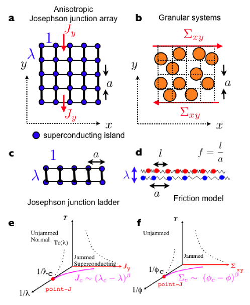
Figure 1: Highly frustrated anisotropic JJA and granular materials. We consider an array of Josephson junctions on a square lattice with linear size $L$ (in the unit of lattice spacing $a$) (a). The ladder version of the JJA model (c) can be mapped onto a friction model (d). The control parameter corresponding to the number density of granular particles $\phi$ or normal load (f) is the strength of the anisotropy of the Josephson coupling $\lambda$ (e).

The JJA Tinkam ; Teitel-Jayaprakash ; Mooji-group is a network of superconducting islands as depicted in Fig. 1 (a). The phase of superconducting order parameter of the islands at site $i$, $\theta_{i}$, is coupled to its nearest neighbors by the Josephson junctions. External transverse magnetic field $B$ thread the cells in the forms of flux lines each of which carrying a flux quanta $\phi_{0}$. On average each unit cell of the square lattice carries $f=Ba^{2}/\phi_{0}$ flux lines. A flux line threading a unit cell induces a vortex of the phases around the cell much as a dislocation in a crystal. Here $A_{ij}$ is the vector potential. The static and dynamic properties of the JJA under transverse magnetic field are known to be described to a good accuracy by the energy term associated with the Josephson couplings Tinkam ; Teitel-Jayaprakash ,

$$H=\sum_{<i,j>}K_{ij}E_{ij}(\theta_{i}-\theta_{j}-A_{ij})\qquad E_{ij}(\psi)=-\cos(\psi)$$ (1)

where $K_{ij}$ is the strength of the Josephson coupling.

In mid 80’s a tantalizing possibility of a superconducting glass in the JJA has been raised by Halsey Halsey : if the transverse magnetic field is tuned in such a way that the number density $f$ of the vorticies takes irrational values, a glassy state may be realized at low temperatures because the vorticies may not be able to form periodic structures called vortex lattices which are analogous to ordered structures of dislocations in Frank-Kasper phases. It has been argued that the frustration due to the gauge field like $A_{ij}$ in Eq. (1) mimics geometric frustration in structural glasses (see Tarjus-review for a review on the perspective on the frustration-based point of view on the glass transition). Indeed equilibrium relaxations were similar to the primary relaxation observed in typical fragile supercooled liquids Lee-Kim ; Lee-Kim-Lee . Now recent studies appear to convincingly suggest that the putative (thermal) liquid-glass transition is actually taking place only at zero temperature exhibiting diverging length scale(s) Park-Choi-Kim-Jeon-Chung ; Granato ; Granato2 . We note that all these observations are made on systems in which the Josephson couplings $K_{ij}$ are isotropic.

As stated at the beginning our key observation is that the anisotropy of the Josephson coupling $K_{ij}$ is a relevant variable and plays the role similar to the particle normal load or density in the jamming of granular materials Jamming-Book (Fig. 1 (a)(b)). We parametrize the anisotropic coupling as,

$$K_{ij}=\left\{\begin{array}[]{cc}1&\mbox{for $\langle i,j\rangle$ directed along the $x$ axis}\\ \lambda&\mbox{for $\langle i,j\rangle$ directed along the $y$ axis}\\ \end{array}\right.$$ (2)

Such an anisotropic JJA can be realized experimentally by controlling the width of the junctions anisotropic-JJA . Let us also note that similar anisotropic couplings arise naturally also in cuprate high-Tc superconductors Hu-Tachiki and charge-density-wave systems Nogawa-Nemoto .

Another key observation is that the model Eq. (1) can be slightly modified to build an effective Eulerian model for rheology of granular systems under horizontal shear as shown in Fig. 1 (b). We assume that particles move predominantly parallel to the direction of driving ($x$ axis) confined within the horizontal layers without passing over others in the same layer. Then the variable $\theta_{i}$ can be interpreted as a phase variable Yoshino by which the number density of particles within the $i$-th cell is described, for instance, as $\rho_{i}=(1/2)(1+\cos(\theta_{i}))$. Here the size $a$ of the cell corresponds to the typical scale of particles and their mutual distances continuous-limt . The sinusoidal intra-layer couplings $E_{ij}(\psi)=-\cos(\psi)$ in Eq. (1) are replaced by elastic couplings $E_{ij}(\psi)=\psi^{2}/2$ while the sinusoidal form is kept for the inter-layer couplings to allow phase slips between different layers. Let us call such a model as semi-elastic model. Here the vorticies represent dislocations. We assume that the geometrical frustration induced by the gauge field $A_{ij}$ mimics real frustrations in granular and other glassy systems Tarjus-review . In the absence of the frustration ($A_{ij}=0$) the semi-elastic model exhibits a non-linear rheology associated with a Kosterlitz-Thouless transition at finite temperatures Yoshino .

The dynamics of the models can be described by the equation of motion,

$$\frac{d\theta_{i}}{dt}=v_{i},\qquad\qquad m\frac{dv_{i}}{dt}=-\frac{\partial H}{\partial\theta_{i}}+F_{i}$$ (3)

Here the frictional force $F_{i}$ is given by $F_{i}=-\gamma\sum_{j}(v_{i}-v_{j})$ with the summation taken over the $4$ nearest neighbours of $i$. This equation of motion is nothing but the standard resistively and capacitively shunted junction (RCSJ) dynamics Tinkam ; Granato , which can also be viewed as a model for rheology of the layered systems Yoshino . For simplicity we choose mass (capacitance) $m=1$, damping constant (resistance) $\gamma=1$. Here we focus only on the zero temperature dynamics. Appropriate thermal noise can be added to Eq. (3) for finite temperature dynamics. For the semi-elastic model we assumed two different types of constitutive relations for the frictional force $F_{i}$ in Eq. (3): (1) Newtonian viscous friction $F_{i}=-\sum_{j}(v_{i}-v_{j})$ and (2) Bagnold’s friction Bagnold ; Mitarai-Nakanishi $F_{i}=-\sum_{j}|v_{i}-v_{j}|(v_{i}-v_{j})$ where the sum is taken over the nearest neighbours on the two adjacent layers.

The anisotropic coupling Eq. (2) can be motivated by recalling a well known problem in the science of friction. A class of friction models related to the Frenkel-Kontorova model FK-review is known to exhibit the so called Aubry’s transition aubry which is a kind of jamming transition at zero temperature. In Fig. 1 (d) we display a friction model proposed by Matsukawa and Fukuyama matsukawa-fukuyama which consists of two layers of atoms representing surfaces of two different solids. In general the ratio (winding number) $f=l/a$ of the mean atomic spacings on the two different materials takes irrational values. The atoms in the same layers are connected to each other by springs while those on different layers interact with each other via short-ranged interactions of strength $\lambda$, which mimic the normal load. In the weak coupling regime $\lambda<\lambda_{c}$, the two chains of atoms slide smoothly with respect to each other thanks to the incommensurability. On the other hand in the strong coupling regime $\lambda>\lambda_{c}$ the system is pinned into amorphous metastable states and a finite static frictional force or yield stress emerges. Note that an anisotropic JJ ladder Denniston-Tang-ladder shown in Fig. 1 (c) which consist of two horizontal layers can be viewed as an Eulerian formulation of the friction model. The irrational winding number $f$ can be identified with the irrational number density $f$ of vorticies in a unit cell in the JJ ladder.

An important consequence of the anisotropic coupling Eq. (2) in 2 (and higher) dimensions is that the effective repulsive long-ranged interactions between the vorticies become anisotropic. For $\lambda<1$ the vorticies will tend to align vertically since the repulsive force is stronger along the $x$ axis, which make it much harder for the vorticies to move along the $y$ axis, i.e. the direction with weaker coupling. Of course the situation becomes reversed for $\lambda>1$.

The rigidity of the system can be probed by applying an external current just as external shear stress is applied on a solid. What corresponds to the shear stress $\Sigma_{xy}$ along the $x$ axis (Fig. 1 (b)) is the vertical external electric current $J_{y}$ (Fig. 1 (a)) Yoshino . Then vorticies (dislocations) are driven along $x$ axis by the Lorentz force. The resultant electric field $E_{y}$ which is proportional to the average velocity of the vorticies corresponds to the shear-rate $\dot{\Gamma}_{xy}$ which measures the rate of plastic deformations in rheology. If the vorticies don’t move significantly resisting against the Lorentz force, the energy dissipation is negligible and the system remains macroscopically superconducting. In practice, we apply shear to the system by forcing the top and bottom layers (walls) to move along the opposite directions at constant velocities. We measure the resultant electric field $E_{y}$ (shear-rate $\dot{\Gamma}_{xy}$) defined as the slope of phase velocity $v_{i}$ developed in the system along the $y$ axis. Electric current flowing through a junction from site $i$ to $j$ is defined as $\sin(\theta_{i}-\theta_{j}-A_{ij})$. The currents running through the junctions parallel to $x$ and $y$ axes correspond to the shear stresses $\Sigma_{xx}$ and $\Sigma_{xy}$ respectively in rheology.

By construction of the system, static and dynamic resposes to $J_{x}$ at anisotropy $\lambda$ at $T=0$ is just the same as those to $J_{y}$ with $\lambda^{\prime}=1/\lambda$. Thus in the following we only display results of resposes to $J_{y}$.

We numerically solved the equation of motion Eq. (3) by the 4th order Runge-Kutta method runge-kutta . Periodic boundary condition is imposed along the $x$ axis only. For a given irrational vortex density $f$ we used its rational approximations $p/q$ with integer $p$ and $q$ in systems of sizes $L=nq$ (with $n=1$ or $2$). To explore larger length/time scales we use systematically better approximants to prevent commensurability (or matching) effects. (See APPENDIX A) Before starting measurements, we checked that the velocity profile becomes linear into the $y$ axis without shear-bands and that observed quantities do not depend on the prior shear histories.

Figure 2: Snapshots of vorticies and local electric-currents in the steady states under shear at zero temperature. Vorticies (a-c) tend to align into the direction with weaker coupling. Local electric currents (d-i) exhibit chain-like configurations which are reminiscent of the “force chains” observed in granular materials. The “current-chains” tend to percolate into the direction with weaker coupling. The system size is $L=42$ with $f=8/21$ which approximates $(3-\sqrt{5})/2=0.3819..$. The system is sheared such that the electric field $E_{y}$ (shear rate) is $0.006$.

Shown in Fig. 2 are snapshots of the vorticies and local currents under shear of the anisotropic JJA. Chains of electric currents reminiscent of “force chains” Cate-Wittmer-Bouchaud-Claudin ; Jamming-Book in granular materials can be noticed. The configurations at the isotropic point $\lambda=1$ appear to manifest the diagonal stripe structures found in the ground states halsey-staircase ; gupta ; Denniston-Tang . As expected the vorticies and the electric currents flowing along the trains of vorticies tend to align into the direction with weaker coupling. This observation strongly suggests that a jamming transition takes place at the isotropic point $\lambda_{c}=1$. The system behaves as a fluid (unjammed phase) for $\lambda<\lambda_{c}$ and amorphous solid (jammed phase) for $\lambda>\lambda_{c}$ with respect to $J_{y}$ as depicted in Fig. 1 (e). Furthermore it is interesting to note that the jammed state is inevitably fragile in somewhat similar sense as proposed in the context of granular matters Cate-Wittmer-Bouchaud-Claudin : the system with a given $\lambda$ can resist against shear only into one direction (i. e. superconducting). Thus we may call such a state of matter as fragile vortex matter in the same spirit of Cate-Wittmer-Bouchaud-Claudin . The qualitative features are essentially the same in the semi-elastic model except that vorticies move only into $x$ axis in the latter model.

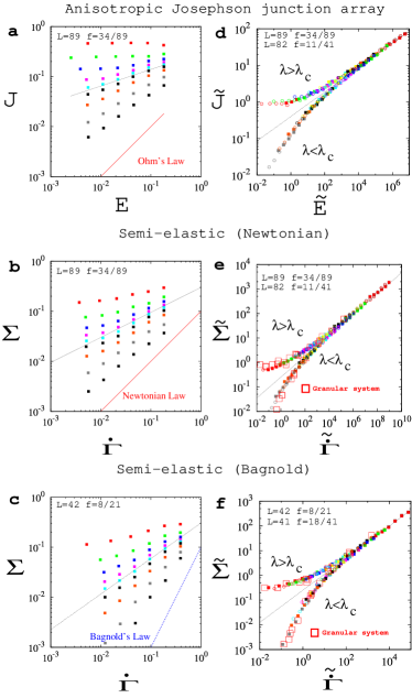
Figure 3: Current-voltage curves and flow curves. The left panels (a,b,c) show the current-voltage of the JJA (a), flow curves of the semi-elastic model with Newtonian friction (b) and that with Bagnold friction (c). The right panels (d,e,f) are corresponding scaling plots. The master-curves obtained in numerical simulations of 2 dimensional granular systems Hatano-Yoshino with coefficient of restitution equal to/smaller than $1$ are included in (e) and (f) respectively. In the right panels (a,b,c) the strength of the inter-layer coupling $\lambda$ is varied as $\lambda=0.625,0.75,0.875,0.95,1.0,1.050,1.125$ and $1.5$ from the bottom to the top curves. The dotted lines are power law fits to the curve at $\lambda_{c}=1$ which yields $1-\alpha=\beta/\Delta=0.34(3)$ (JJA),$0.43(6)$ (semi-elastic-Newtonian) and $0.65(4)$ (semi-elastic-Bagnold). The scaling plots in the right panels (d,e,f) show $\tilde{J}\propto J/(\lambda-\lambda_{c})^{\beta}$ vs $\tilde{E}\propto E/(\lambda-\lambda_{c})^{\Delta}$ and $\tilde{\Sigma}\propto\Sigma/(\lambda-\lambda_{c})^{\beta}$ vs $\tilde{\dot{\Gamma}}\propto\dot{\Gamma}/(\lambda-\lambda_{c})^{\Delta}$ with $\lambda_{c}=1$. The resultant values of the exponent $\Delta$ which give best scaling collapse are $3.5$ (JJA),$4.2$ (semi-elastic-Newtonian)and $2.4$ (semi-elastic-Bagnold). In the left panels (a,b,c) $f=34/89$ is used which approximates $(3-\sqrt{5})/2$. In the right panels (d,e,f) data of $f$ which approximate $2-\sqrt{3}$ (d,e) and $(5-\sqrt{17})/2$ (f) are also included. We have checked that finite size effects and commensurability effects are not significant within the range of shear-rates used here. In the semi-elastic-Bagnold model (f) the system size is limited to avoid strong shear-banding effects. The scaling functions of the granular systems (e,f) are obtained by plotting $\tilde{\Sigma}\propto\Sigma/(\phi-\phi_{c})^{\beta^{\prime}}$ vs $\tilde{\dot{\Gamma}}\propto\dot{\Gamma}/(\phi-\phi_{c})^{\Delta^{\prime}}$ with $\phi_{c}=0.8415$ (random close packing density in two dimensions) and appropriate exponents $\beta^{\prime}$ and $\Delta^{\prime}$.

The current-voltage curves obtained at different values of the coupling $\lambda$ are displayed in Fig. 3 (a). At stronger coupling $\lambda>1$ it appears that a non-zero critical current $J_{c}(\lambda)=\lim_{E\to 0}J(E,\lambda)$ exists, which becomes larger with increasing $\lambda$. This means that the Lorentz force does not drive the vorticies significantly so that the system remains macroscopically superconducting along the $y$ axis at strong enough coupling $\lambda$. The finite critical current corresponds to the yield stress $\Sigma_{c}$ in rheology. The disordered configurations of vorticies shown in Fig. 2 suggests that the system is an amorphous glassy state of vorticies. On the other hand, at smaller coupling $\lambda<1$ and low enough $E$ the Ohm’s law $J=\sigma(\lambda)E$ holds with finite linear conductivity $\sigma(\lambda)$ which becomes larger with increasing $\lambda$. Thus the vorticies can flow easily producing significant energy dissipation at weak enough coupling $\lambda$. At the isotropic point $\lambda=1$, we find a power law $J\propto E^{1-\alpha}$ with $1-\alpha=0.34(3)$. This corresponds to the so called shear-thinning behaviour ($\alpha>0$) in rheology rheologybook .

The above results strongly indicate that $\lambda_{c}=1$ is the critical point of a 2nd order phase transition at zero temperature. This is supported by a good scaling collapse of the data onto a master curve as shown in Fig. 3 (d). Our scaling ansatz is similar in spirit to the ones used for the usual normal-to-superconducting phase transition at finite temperatures WGI ; FFH which can also be reinterpreted in the context of rheology Yoshino ,

$$J=(\lambda-\lambda_{c})^{\beta}\tilde{J}\left(\frac{E}{(\lambda-\lambda_{c})^{\Delta}}\right)$$ (4)

The scaling function (master flow curve) is expected to behave asymptotically as $\tilde{J}(x)\propto x$ for small enough $x$ in the Ohmic phase ($\lambda<\lambda_{c}$) and $\lim_{x\to 0}\tilde{J}(x)\to{\rm const}$ in the superconducting phase ($\lambda>\lambda_{c}$). The scaling ansatz Eq. (4) implies 1) the linear conductivity diverges as $\sigma(\lambda)\propto(\lambda-\lambda_{c})^{-(\Delta-\beta)}$ for $\lambda\to\lambda_{c}^{-}$, 2) the critical current vanishes as $J_{c}(\lambda)\propto(\lambda-\lambda_{c})^{\beta}$ for $\lambda\to\lambda_{c}^{+}$ and 3) the critical behaviour $\tilde{J}(x)\propto x^{1-\alpha}=x^{\beta/\Delta}$ sets-in for large $x$. Here we used the notations reflecting the analogy with the equilibrium critical behaviour of ferro-magnets under magnetic field as noticed by Wolf, Gubser and Imry WGI : the shear plays the role of symmetry breaking field like the magnetic field and the critical current emerges as an order parameter like the magnetization (see Otsuki-Sasa for a similar argument in the context of rheology). As shown in Fig. 3, we find our scaling ansatz works well with $\lambda_{c}=1$. We have checked that the universality does not depend on the use of different irrational values of $f$ as demonstrated in Fig. 3 (d).

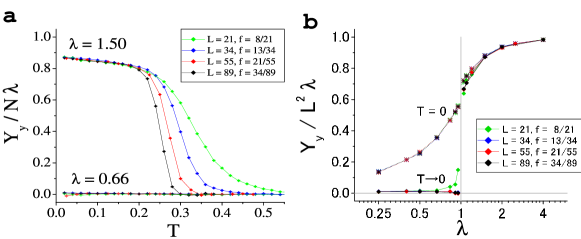
Figure 4: Static helicity (shear) modulus in the anisotropic JJA. The helicity modulus $Y_{y}$ is obtained as equilibrium ensemble averages of the susceptibilities against twists along the $y$ axis. (a) Temperature $T$ and size $L$ dependence of the helicity modulus $Y_{y}$ and (b) its extrapolation to $T\to 0$. In (b) helicity modulus at $T=0$ is also shown. The values of $f$ used here approximate $(3-\sqrt{5})/2$. The periodic boundary condition is imposed along both $x$ and $y$ aixes on the system of size $N=L\times L$. The standard simulated annealing method is used to generate the equilibrium ensemble (appendix B).

Let us note that the critial current discussed above $J_{c}(\lambda)=\lim_{E\to 0}J(E,\lambda)$ corresponds to the dynamical yield stress in rheology. On the other hand one can also define the quasi-static critical current(s) needed to move out of a generic metastable state (or the ground state), corresponding to the static yield stress in rheology, as studied by Teitel and Jayaprakash Teitel-Jayaprakash on the JJA. In practice one can consider athermal quasi-static processes similar to those used in some recent studies on amorphous solids anael ; anael2 ; barrat : starting from a metastable state reached from a random initial configuration by a qunech, i. e. deterministic energy descent process, the system is subjected to externally induced uniform strain $\delta$ (See Eq. (6)) which is increased step by step. The system relaxes down to an energy minimum by the energy descent process after each small increment of $\delta$. As the result one finds that the current $J(\delta)$ is a sawtooth-like function of $\delta$: piecewise linear lines corresponding to elastic deformations broken by yield points at plastic events, as observed in amorphous solids anael ; anael2 ; barrat . A critical current can be defined as the value of the current just before reaching a yield point. In Halsey Halsey has found that typical value of such quasi-static critical current $J_{c}^{\rm static}(1)$ is finite in the isotropic system $\lambda=1$. Moreover we found that $J_{c}^{\rm static}(\lambda)$ varies smoothly with $\lambda$ and remains finite even in the unjammed phase $\lambda<1$ found above comment-on-TJ-conjecture . Our data of $J(E,\lambda)$ in the flow curves becomes smaller than $J_{c}^{\rm static}(\lambda)$ meaning that the quasi-static current needed to move out of a generic metastable state and dymamic critical currents are distinct in the present system. Quite interestingly we observed that the flow curves become strongly dependent on strain histories below $J_{c}^{\rm static}(\lambda)$. In practice we had to use an annealing procedure to obtain stationary data: decrease $E$ (shear rate) very slowly down to the target one. Slower shear rates are needed to investigate smaller current $J$ (shear stress) regions. Note that no annealing is performed in the athermal quasi-static process discussed above. These observations suggest ruggedness of the energy landscape of the present system.

We also investigated static response to shear (See APPENDIX B for the details.). As shown in Fig. 4, the static helicity (shear) modulus is very sensitive to the anisotropy. The figure shows that the helicity modulus remains zero down to $T\to 0$ for $\lambda<1$ and becomes finite for $\lambda>1$. Thus at $T=0$ the isotropic point appears to be the critical point $\lambda_{c}=1$ being consistent with the dynamic response discussed so far. Here let us recall again that just by symmetry, helicity modulus $Y_{x}/\lambda$ at anisotropy $\lambda$ is identical to $Y_{y}/\lambda^{\prime}$ at $\lambda^{\prime}=1/\lambda$. Then the fact that $\lambda_{c}=1$ means that this system is quite exotic: fragile vortex matter which behaves as a solid with respect to shear along one direction but liquid for the other direction.

Another remarkable feature is the difference of the static helicity modulus between $T=0$ and $T\to 0$ limit which can be seen in Fig. 4 b). The helicity modulus at $T=0$ only reflects local stability of energy minima. This difference suggests the existence of certain softmodes with vanishingly small energy gaps as discussed in APPENDIX B. This observation suggests that the vortex liquid behaviour at $T=0$ is realized by some non-trivial softmodes due to frustrations.

Based on the above results we obtain the jamming phase diagram of the anisotropic JJA as shown in Fig. 1 (e) which is surprisingly similar to that of granular systems shown in Fig. 1 (f) Liu-Nagel ; Jamming-Book ; Nagel-group .

Now let us turn to the semi-elastic model. In Fig. 3 (b,c), we display the flow curves of the semi-elastic model. The shear-stress due to the inter-layer coupling terms also obeys the Newtonian or Bagnold scaling for small $\lambda$ at low enough $\dot{\Gamma}$. Flow curves at large $\lambda$ suggests existence of non-zero yield stresses $\Sigma_{c}(\lambda)=\lim_{\dot{\Gamma}\to 0}\Sigma(\dot{\Gamma},\lambda)$. We find again a power law behaviour $\Sigma\propto(\dot{\Gamma})^{1-\alpha}$ with $\alpha>0$ (shear-thinning) at $\lambda=1$. Indeed the scaling ansatz Eq. (4) (with $E\to\dot{\Gamma}$ and $J\to\Sigma$) works well again assuming $\lambda_{c}=1$ and the universality does not depend on the different irrational values of $f$ (Fig. 3 (e,f)).

Recent numerical simulations of granular materials with/without strong dissipation at the particle level (coefficient of restitution smaller than/equal to $1$) have found Bagnold/Newtonian scalings in the fluid phase and different critical exponents Xu-Hern ; Hatano-Otsuki-Sasa ; Olsson-Teitel ; Hatano ; Hatano-Yoshino . Quite interestingly the values of the shear-thinning exponent $1-\alpha$ found in our semi-elastic model with Bagnold/Newtonian frictions are $0.63$ and $0.42$ respectively in agreement with the exponents of the corresponding two-dimensional granular systems with repulsive linear spring forces between the particles. For a comparison master flow curves of the granular systems Hatano-Yoshino are displayed in Fig. 3 (e,f). Quite remarkably the functional forms of the master flow-curves themselves agree very well.

In the present paper we focused on the responses of the systems to shear at zero temperature. Recent studies at the isotropic point $\lambda=1$ at finite temperatures suggest critical behaviour with $T\to 0$, i. e. $T_{c}(\lambda=1)=0$ with diverging length scales Park-Choi-Kim-Jeon-Chung ; Granato ; Granato2 . If this would be confirmed, our system would provide a fascinating example where both the (thermal) liquid-glass transition and the (athermal) unjamming-jamming transition take place at the same thermodynamic point, $T=0$ and $\lambda_{c}=1$, demonstrating deep connection between the two transitions. At least in this system, the jamming and glass transitions appears to be the two sides of a coin. It would be interesting to further explore this connection to make this statement more substantial. A related interesting question is whether or not the jamming (glass) phase survives at finite temperatures. Then the possibilities are 1) the jamming point at $\lambda=1$ at $T=0$ is an isolated critical point or 2) a critical line $T_{c}(\lambda)$ starts from the jamming point as shown in Fig. 1 (e). Our preliminary study points to the latter possibility.

We emphasize that the jamming transition here is purely due to geometrical frustration which is free from any quenched disorder in sharp contrast to the conventional vortex glasses FFH for which presence of random pinning centers are crucial. This is a much awaited, concrete example of a jamming-glass transition purely due to geometrical frustration Tarjus-review . It is tempting to speculate that similar phenomena may exist in frustrated magnets such as antiferromagnets on triangular, kagome and pyrochlore lattices pyrochlore . We also note that it will be important and interesting to clarify how quenched disorders, which may not be completely avoided in experimental JJAs, come into play.

Acknowledgement We thank T. Hatano, H. Hayakawa, H. Kawamura, K. Nemoto, H. Matsukawa, T. Ooshida, M. Otsuki, S. Sasa and S. Yukawa for stimulating discussions. The authors thank the Supercomputer Center, Institute for Solid State Physics, University of Tokyo for the use of the facilities. This work is supported by Grant-in-Aid for Scientific Research on Priority Areas ”Novel States of Matter Induced by Frustration” (1905200*) and by 21st Century COE program Topological Science and Technology .

Appendix A Rational approximants and commensurability effects

The purpose of the present paper is to analyzed physical properties of the anisotropic JJA with irrrational vortex density $f$. However in order to use the periodic boundary condition we had to use rational approximants for a given irrational number. Here we explain how commensurability or matching effects emerge and explain how we avoid them in the present study.

For convenience we considered a family of irrational numbers called quadratic irrationals. A well known example is the golden mean $(1+\sqrt{5})/2$. Their rational approximants $f_{n}$ can be generated systematically by solving a simple recursion formulae,

$$f_{n}=\frac{a_{n-1}}{a_{n}}\qquad Aa_{n+1}=Ba_{n}+Ca_{n-1}$$ (5)

where $A$, $B$ and $C$ are integer coefficients and $a_{0}$, $a_{1}$ are certain integers. It is easy to verify that the $f_{n}$s converge to an irrational number $f\equiv\lim_{n\to\infty}f_{n}$ which is a solution of a quadratic equation $Cf^{2}+Bf-A=0$. For instance the golden mean $(1+\sqrt{5})/2$ can be obtained using the Fibonacci numbers $a_{n}$ which satisfy the above recursion formula with $A=B=C=1$ and $a_{2}=a_{1}=1$. Examples of rational approximants $f_{n}$ are shown in Fig. 5 (a) which approximate $(3-\sqrt{5})/2$. They are generated by solving Eq. (5) recursively with $A=1$, $B=3$, $C=-1$ and $a_{2}=a_{1}=1$. It can be seen that the approximation becomes better such that $|f-f_{n}|$ becomes smaller as $n$ increases.

In Fig. 5 (b) flow curves of the anisotropic JJA model at $T=0$ with the rational vortex densities $f_{n}$ are shown. Apparently flow curves of a given anisotropy $\lambda$ converge to a limiting curve as $n$ is increased. We regard the latter as the flow curve of $f=(3-\sqrt{5})/2$ at anisotropy $\lambda$. It can also be seen that flow curves of a given approximant $f_{n}$ closely follow the limiting curve at large enough electric field $E$ (shear rate $\dot{\Gamma}$) and deviate from it at lower $E$. In the $n$ dpendent branches the current $J(E)$ (shear force $\Sigma$) tends to saturate to some finite values in $E\to 0$ limit, i. e. critical current $J_{c}(\lambda,f_{n})$ (yield stress $\Sigma_{c}$) which decreases with increasing $n$ being consistent with the prediction by Teitel and Jayaprakash Teitel-Jayaprakash (see also halsey-staircase ). The latter behaviour suggests that a periodic vortex lattice (crystal) Teitel-Jayaprakash ; halsey-staircase ; Mooji-group ; gupta associated with a given rational vortex density $f_{n}$ is formed and that the latter dictates physical properties of the system at length/time scales larger than its lattice spacing. Thus we expect the so called ’Bingham fluid’ behaviour (fluid with finite yield stress) cannot be avoided for any small $\lambda$ for fixed $n$ and that the genuine fluid phase at $T=0$ is realized only for truly irrational vortex densities. On the other hand the above results shown in Fig. 5 (b) suggest that physical properties at short enough length/time scales, which are $n$ independent, reflect those properties of irrational $f$. Thus our strategy in the present work is to choose large enough $n$ such that the $n$ dependency do not become relvant within the range of $E$ (shear rate $\dot{\Gamma}$) we choose to work on.

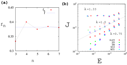
Figure 5: Rational approximants and commensurability effects on the flow curves. (a) Approximants $f_{n}$ for $f=(3-\sqrt{5})/2$. (b) Data of the flow curves of the anisotropic JJA at $T=0$ with $f=1/3$ ($L=42$), $2/5$ ($40$), $3/8$($40$), $5/13$ ($39$) and $8/21$ ($42$) are shown. The dotted straight line represents the power law $J\propto E^{0.35}$ at the critical point.

Appendix B Static response with respect to shear

To study static response to shear along, say $y$ axis, it is useful to consider a modified Hamiltonian,

$$H=-\sum_{<i,j>||e_{x}}\cos(\phi_{ij})-\lambda\sum_{<i,j>||e_{y}}\cos(\phi_{ij}-\delta),\qquad\phi_{ij}\equiv\theta_{i}-\theta_{j}-A_{ij}$$ (6)

with periodic boundary conditions along both $x$ and $y$ axes. Here $e_{x}$ and $e_{y}$ are unit vectors along $x$ and $y$ axes. This is equivalent to consider a system with twisted boundary condition (shear) with total phase difference $L\delta$ forced across the system along the $y$ axis Teitel-Jayaprakash .

In equilbrium at temperature $T$ the free-energy $F(\delta)$ of the system under shear strain $\delta$ can be defined. Then the static helicity modulus $Y_{y}$ is defined as,

$$Y_{y}\equiv\frac{\partial^{2}F}{\partial\delta^{2}} =\lambda\sum_{<i,j>||e_{y}}\langle\cos(\phi_{ij})\rangle$$ (7)

$$-\lambda\beta\sum_{<i,j>||e_{y}}\sum_{<k,l>||e_{y}}\left(\langle\sin(\phi_{ij})\sin(\phi_{kl})\rangle-\langle\sin(\phi_{ij})\rangle\langle\sin(\phi_{kl})\rangle\right)$$

where $\beta\equiv 1/(k_{B}T)$ and $\langle\ldots\rangle$ are equilibrium thermal averages at finite temperature $T$. The 1st term on the r. h. s reflects direct elastic response around energy minima with respect to a small externally induced shear strain. On the other hand, the 2nd term reflects relaxation of the system against the external strain at finite temperatures.

Here the distinction between $T=0$ and $T\to 0$ is important. At $T=0$ only the 1st term exists. However, the contribution of the 2nd term can remain, in principle, in $T\to 0$ limit if the strength of the thermal fluctuation of the current $\sin(\phi_{ij})$ is $O(T)$. Such a situation can arise if there are soft modes with vanishingly small energy gap such that they remain thermally active at arbitrarily low temperatures.

To obtain the equilibrium ensemble to evaluate the helicity modulus at $\delta=0$, we performed simulations of relaxational dynamics by numerically solving the Langevin equation

$$\frac{\partial\theta_{i}}{\partial t}=-\frac{\partial H}{\partial\theta_{i}}+\sqrt{2T}\xi_{i}(t)$$ (8)

with the Hamiltonian $H$ given in Eq. (1) and $\xi_{i}(t)$ being Gaussian noise with zero mean and unit variance, by the 2nd order Runge-Kutta method. The system is cooled with cooling rates $dT/dt=10^{-10}-10^{-9}$ starting from initial temperature at $T=0.3-1.0$. We have checked that the cooling rate is slow enough by comparing with the results of $4$ times faster cooling rate.

References

- (1) ”Hydrodynamic Fluctuations, Broken Symmetry and Correlation Functions”, D. Foster, (Addison Wesley, Reading, MA 1990).
- (2) ”Rheology: Principles, Measurements, and Applications”, C. W. Macosko, VCH (1994) New York.
- (3) ”Introduction to Superconductivity”, M. Tinkham, Courier Dover Publications (2004).
- (4) H. Yoshino, H. Matsukawa, S. Yukawa and H. Kawamura, J. Phys.: Conf. Ser. 89 012014 (2007).
- (5) M. E. Cates, J. P. Wittmer, J.-P. Bouchaud, and P. Claudin, Phys. Rev. Lett. 81, 1841 - 1844 (1998).
- (6) A. J. Liu and S. R. Nagel, Nature, Volume 396, Issue 6706, pp. 21-22 (1998).
- (7) ”Jamming and Rheology: Constrained Dynamics on Microscopic and Macroscopic Scales”, Ed. A. J. Liu , S. R. Nagel, CRC Press (2001).
- (8) C. S. O Hern, L. E. Silbert, A. J. Liu and S. R. Nagel, Phys. Rev. E 68, 011306 (2003).
- (9) O. Dauchot, G. Marty, and G. Biroli, Phys. Rev. Lett. 95, 265701 (2005).
- (10) N. Xu and C. S. O’Hern, Phys. Rev. E 73, 061303 (2006).
- (11) M. Otsuki, S. Sasa, J. Stat. Mech., L10004 (2006).
- (12) T. Hatano, M. Otsuki and S. Sasa, J. Phys. Soc. Jpn. 76 023001 (2007).
- (13) P. Olsson and S. Teitel, Phys. Rev. Lett. 99, 178001 (2007) .
- (14) T. Hatano, arXiv:0803.2296v4, to appear in J. Phys. Soc. Japan.
- (15) A. S. Keys, A. R. Abate, S. C. Glotzer, D. J. Durian, Nature Physics 3, 260 (2007).
- (16) E. R. Weeks, in ”Statistical Physics of Complex Fluids”, pp. 2-1 – 2-87, eds. S Maruyama & M Tokuyama (Tohoku University Press, Sendai, Japan, 2007).
- (17) S. Teitel and C. Jayaprakash, Phys. Rev. Lett. 51, 1999 (1983).
- (18) H. S. J. van der Zant, H. A. Rijken, and J. E. Mooij, Journal of Low Temperature Physics, 82 67 (1991).
- (19) T. C. Halsey, Phys. Rev. Lett. 55, 1018 (1985).
- (20) G. Tarjus, S. A. Kivelson, Z. Nussinov and P. Viot, J. Phys. Condens. Matters 17 R 1143 (2005).
- (21) B. Kim and S. J. Lee, Phys. Rev. Lett. 78, 3709 (1997).
- (22) S. J. Lee, B. Kim, and J. -R. Lee, Phys. Rev. E 64, 066103 (2001).
- (23) S. Y. Park, M. Y. Choi, B. J. Kim, G. S. Jeon, and J. S. Chung, Phys. Rev. Lett. 85, 3484 - 3487 (2000).
- (24) E. Granato, Phys. Rev. B 75, 184527 (2007).
- (25) E. Granato, Phys. Rev. Lett. 101, 027004 (2008).
- (26) S. Saito and T. Osada, Physica B: Condensed Matter Vol 284-288, 614 (2000).
- (27) X. Hu and M. Tachiki, Phys. Rev. Lett. 80 4044 (1998).
- (28) T. Nogawa and K. Nemoto, Phys. Rev. B 73, 184504 (2006).
- (29) ”The Frenkel-Kontorova Model - Concepts, Methods and Applications”, O. M. Braun and Y. S. Kivshar, Springer (2004).
- (30) M. Peyard and S. Aubry, J. Phys. C: Solid State Phys., 16 (1983) 1593.
- (31) H. Matsukawa and H. Fukuyama, Phys. Rev B. 49, 17286 (1994).
- (32) C. Denniston and C. Tang, Phys. Rev. Lett. 75, 3930 (1995).
- (33) T. C. Halsey, Phys. Rev. B 31, 5728 (1985).
- (34) P. Gupta, S. Teitel, and M. J. P. Gingras, Phys. Rev. Lett. 80, 105 - 108 (1998).
- (35) C. Denniston and C. Tang, Phys. Rev. B 60, 3163 (1999).
- (36) S. A. Wolf, D. U. Gubser and Y. Imry, Phys. Rev. Lett. 42, 324 (1979).
- (37) D. S. Fisher, M. P. A. Fisher and D. A. Huse, Phys. Rev. B 43, 130 (1991).
- (38) R. A. Bagnold, Proceeding of Royal Soceity of London A 225, 49 (1954).
- (39) N. Mitarai, H. Nakanish, Phys. Rev. Lett. 94, 128001 (2005)
- (40) C. Maloney and A. Lemaître, Phys. Rev. Lett. 93, 195501 (2004).
- (41) C. Maloney and A. Lemaître, Phys. Rev. E 74 06118 (2006).
- (42) A. Tanguy, F. Leonforte and J.- L. Barrat, Eur. Phys. J. E 20, 355 (2006).
- (43) These observations suggest that the argument by Teitel-Jayaprakash Teitel-Jayaprakash leading to the vanishing of the quasi-static critical current for irrational cannot be used always. The assumption of smoothness of the variation of the current with respect to the changes of the strain , which underlies the use of the mean-value theorem in Teitel-Jayaprakash , becomes questionable if plastic deformations take place.
- (44) T. Hatano and H. Yoshino, unpublished. Data are obtained by numerical simulations of sheared friction-less poly-disperse soft-disks of various number densities interacting with each other by the linear force. (For the details of the method see Xu-Hern ; Hatano ; Olsson-Teitel .)
- (45) M. J. P. Gingras, C. V. Stager, N. P. Raju, B. D. Gaulin, and J. E. Greedan, Phys. Rev. Lett. 78, 947 (1997).
- (46) It is essential not to lose ’granularity’, which is the source of frustration effects, by naively taking continuous limit . The irrational winding number can be identified with the irrational number density of vorticies in a unit cell in the Josephson junction ladder.
- (47) We integrated Eq. (3) with integration time step of by the 4th order Runge-Kutta method starting from random initial conditions. Initial steps are discarded and the time averages of the observables are taken in the following steps. We checked the latter protocol is sufficient to obtain stationary data within the shear rates and the system sizes used in the following analysis. The results are averaged over independent runs with different random initial conditions.