Dynamic Coulomb blockade in single–lead quantum dots

Abstract

We investigate transient dynamic response of an Anderson impurity quantum dot to a family of ramp–up driving voltage applied to the single coupling lead. Transient current is calculated based on a hierarchical equations of motion formalism for open dissipative systems [J. Chem. Phys. 128, 234703 (2008)]. In the nonlinear response and nonadiabatic charging regime, characteristic resonance features of transient response current reveal distinctly and faithfully the energetic configuration of the quantum dot. We also discuss and comment on both the physical and numerical aspects of the theoretical formalism used in this work.

I Introduction

Dynamics of open electronic systems far from equilibrium has attracted considerable interest in the past few years, since the dynamic processes are closely related to and thus can be used to explore the system properties of interest. It is well known that electron–electron interaction plays a significant role under realistic experimental conditions Lu03422 . Therefore, understanding the electronic dynamics in presence of electron–electron interaction is of fundamental importance to the emerging field of nanosciences.

So far theoretical work has focused mostly on steady or quasi–steady state dynamics, which however may contain only partial information on the system of study. Consider, for example, a quantum dot (QD) as depicted in Fig. 1(a), with two Zeeman levels of $\epsilon_{\uparrow}<\epsilon_{\downarrow}$, in contact with a single electrode. Under the quasi–steady state charging condition, the applied voltage raises the electrode chemical potential ($\mu$) adiabatically. The first charging electron occupies exclusively the energetically favorable spin–up level, while the second one that occupies the spin–closed double occupation state requires an excess energy to overcome the static on–dot Coulomb blockade; see Fig. 1(b). Apparently, the steady–state study offers rather incomplete information, as the single occupation of spin–down state is dark here.

In this work, we resort to transient dynamics of the system, by applying a time–dependent external voltage to the system, i.e., $\mu$ varies explicitly in real time, and analyzing the resulting nonadiabatic charging process. It is expected that all transitions within the range of applied voltage will be manifested through the system dynamic properties. Specifically, we consider a single–lead Anderson impurity QD driven by a family of ramp–up external voltages, by exploiting the hierarchical equations of motion (HEOM) theory for open electronic dynamics and transient current Jin08234703 . In Sec. II we briefly describe the theoretical and computational aspects. We demonstrate in Sec. III that the transient dynamics reveals sensitively and faithfully the QD energetic configuration. Section IV concludes this work.

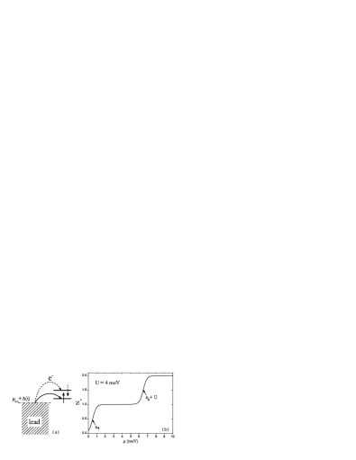
Figure 1: (a) An interacting QD coupled to a single lead with a time–dependent chemical potential ${\mu}(t)=\mu_{\rm eq}+\Delta(t)$. (b) The steady–state number of electrons on QD, $N_{e}$, as a function of ${\mu}$. Other parameters adopted are (in unit of meV): $\epsilon_{\uparrow}=0.5$, $\epsilon_{\downarrow}=2.5$, $U=4\,$, $T=0.2$, the QD–lead coupling strength $\Gamma=0.05$ and bandwidth $W=15$. See Sec. III.1 for details.

II Methodology

We implement a HEOM formalism, which is formally exact for dynamics of an arbitrary non–Markovian dissipative system interacting with surrounding baths Jin08234703 ; Xu05041103 ; Xu07031107 ; Jin07134113 . From the perspective of quantum dissipation theory, the electronic dynamics of an open system is mainly characterized by the reduced system density matrix $\rho(t)\equiv\mbox{tr}_{{}_{\rm B}}\rho_{{}_{\rm T}}(t)$ and the transient current through the coupling leads. Here $\rho_{{}_{\rm T}}(t)$ is the total density matrix of the entire system, and $\mbox{tr}_{{}_{\rm B}}$ denotes a trace over all lead degrees of freedom. The final HEOM is cast into a compact form of Jin08234703

$$\dot{\rho}_{\sf n}=-[i\mathcal{L}+\gamma_{\sf n}(t)]\rho_{\sf n}+\rho_{\sf n}^{{}_{\{-\}}}+\rho_{\sf n}^{{}_{\{+\}}}.$$ (1)

Here, $\mathcal{L}\,\cdot\equiv[H(t),\cdot\,]$ is system Liouvillian (setting $\hbar\equiv 1$). The basic variables of Eq. (1) are $\rho(t)$ and associated auxiliary density operators (ADOs) $\rho_{\sf n}(t)$, where ${\sf n}$ is an index set covering all accessible derivatives of the Feynman–Vernon influence functional Fey63118 .

For a single–level QD coupled to a single lead, the lead correlation function can be expanded by an exponential series via a spectral decomposition scheme Tan906676 ; Mei993365 ; Yan05187 . In this case ${\sf n}$ involves an $\tilde{n}$–fold combination of ($\sigma,s,m$), which characterizes the exponential series expansion with $\sigma=\pm$, $s$ the spin, and $m$ the index of exponents, respectively. Therefore, in Eq. (1) $\rho_{\sf n}|_{\tilde{n}=0}=\rho(t)$ with $\gamma_{\sf n}|_{\tilde{n}=0}=\rho_{\sf n}^{{}_{\{-\}}}|_{\tilde{n}=0}=0$; $\rho_{\sf n}|_{\tilde{n}>0}$ is an ADO at the $\tilde{n}^{{\rm th}}$–tier; $\gamma_{\sf n}(t)$ collects all the related exponents along with external voltages, to $\rho_{\sf n}(t)$; and $\rho_{\sf n}^{{}_{\{-\}}}$ and $\rho_{\sf n}^{{}_{\{+\}}}$ are the nearest lower– and higher–tier counterparts of $\rho_{\sf n}$, respectively. In particular, the $1^{\rm st}$–tier ADOs, $\rho_{\sf n}(t)|_{\tilde{n}=1}=\rho^{\sigma}_{sm}(t)$, determine exclusively the transient current of spin–$s$ through the lead as Jin08234703

$$I_{s}(t)\equiv-\mbox{tr}_{{}_{\rm T}}\!\left[\hat{N}_{s}\dot{\rho}_{{}_{\rm T}}(t)\right]=-2\,\mbox{Im}\sum_{m}\mbox{tr}\!\left[a_{s}\,\rho^{+}_{sm}(t)\right].$$ (2)

$\hat{N}_{s}$ is the lead total–occupation operator of spin $s$; $a_{s}$ is the system annihilation operator of spin $s$; and $\mbox{tr}_{{}_{\rm T}}$ and tr denote trace operations over the total system and reduced system degrees of freedom, respectively. Since there is only one coupling lead, the displacement current at every time $t$ is simply $-\!\sum_{s}I_{s}(t)$; thus the Kirchhoff’s current law retains Pol05161302 ; Pol07205308 . The present HEOM–based quantum transport theory admits classical geometric capacitors or capacitive coupling to a gate electrode. The associated displacement current can then be evaluated readily, leading to the conservation of total current Pol05161302 ; Pol07205308 ; Fra03471 . Gauge invariance Pol05161302 ; Pol07205308 ; Ped9812993 is also guaranteed at all time, as it can be seen from the form of the $0^{\rm th}$–tier of the HEOM Jin08234703 .

It has been proved Jin08234703 that for a noninteracting QD, the HEOM (1) is exact with a finite terminal tier of $\tilde{n}_{\rm max}=2$; while for an interacting QD, in principle an infinite hierarchy is required for the exact transient dynamics. In practice a truncation scheme is inevitable. In this work a straightforward truncation scheme is adopted; that is to set all the higher–tier ADOs zero: $\rho_{\sf n}|_{\tilde{n}>N_{\rm trun}}=0$, with $N_{\rm trun}$ the preset truncation tier. This scheme leads to a systematic improvement of results as $N_{\rm trun}$ increases, i.e., by inclusion of higher–tier ADOs, as verified by extensive numerical tests. For a moderate system–lead coupling strength $\Gamma<5\,T$, quantitatively accurate (if not exact) dynamics is obtained with $N_{\rm trun}=2$, where $T$ is the temperature in the unit of Boltzmann constant (i.e., $k_{B}=1$). A higher $N_{\rm trun}$ means a drastic increase in computational cost. Therefore, considering the tradeoff between numerical accuracy and computational efforts, all the following calculations are carried out with $N_{\rm trun}=2$ by confining the ratio $\Gamma/T$ less than $5$; see Sec. IV for further discussions.

The composite system of interest is described by the Anderson impurity model And6141 , with its Hamiltonian $H_{{}_{\rm T}}$ expressed as

$$H_{{}_{\rm T}}=H+h_{{}_{\rm B}}+H_{{}_{\rm SB}}.$$ (3)

$H$ represents the interacting QD of our primary interest:

$$H=\epsilon_{\uparrow}\hat{n}_{\uparrow}+\epsilon_{\downarrow}\hat{n}_{\downarrow}+U\,\hat{n}_{\uparrow}\hat{n}_{\downarrow}.$$ (4)

Here, $\epsilon_{s}$ is the energy of the spin–$s$ ($\uparrow$ or $\downarrow$) state, $\hat{n}_{s}\equiv a^{\dagger}_{s}a_{s}$ the system occupation–number operator of spin $s$, and $U$ the on–dot Coulomb interaction strength. In Eq. (3), $h_{{}_{\rm B}}=\sum_{k}\sum_{s}\epsilon_{ks}\,\hat{n}_{ks}$ describes the noninteracting coupling lead, with $\epsilon_{ks}$ being the energy of its single–electron state $k$ of spin $s$, and $\hat{n}_{ks}\equiv d_{ks}^{\dagger}d_{ks}$ the lead occupation–number operator. The QD–lead coupling is given by $H_{{}_{\rm SB}}=\sum_{k}\sum_{s}t_{ks}\,d^{\dagger}_{ks}a_{s}+{\rm H.c.}$, where $t_{ks}$ is the coupling matrix element between the lead state $k$ and the QD–level, both with spin $s$. The widely used Drude model is adopted to capture the coupling lead, i.e., a Lorentzian spectral density function of $J(\epsilon)=\Gamma W^{2}/(\epsilon^{2}+W^{2})$, with $W$ characterizing the lead bandwidth.

We consider explicitly the scenario depicted in Fig. 1(a). A ramp–up voltage $V(t)$ is applied to the coupling lead at $t=0$, which excites the QD out of equilibrium. The lead energy levels are shifted due to the voltage, $\Delta(t)=-eV(t)$, with $e$ being the elementary charge, and so is the lead chemical potential $\mu(t)=\mu_{\rm eq}+\Delta(t)$. $\mu_{\rm eq}$ is the equilibrium lead Fermi energy, which is set to zero hereafter, i.e., $\mu_{\rm eq}=0$. Under a ramp–up voltage, $\Delta(t)$ varies linearly with time until $t=\tau$, and afterwards is kept at a constant amplitude $\Delta$:

$$\Delta(t)=\left\{\begin{array}[]{lc}\Delta\,t/\tau,&0\leq t\leq\tau\\ \ \ \Delta,&t>\tau\end{array}\right..$$ (5)

By tuning the duration parameter $\tau$, the family of ramp–up voltage covers three distinct regimes: (A) The adiabatic limit at $\tau\rightarrow\infty$; (B) the intermediate range with a finite $\tau$; and (C) the instantaneous switch–on limit corresponding to $\tau\rightarrow 0^{+}$. These three regimes are individually explored and elaborated in the subsections of Sec. III.

The work flow of our numerical procedures are briefly stated here, while details to be published elsewhere. (a) The lead correlation function is expanded by exponential functions, and hence establishes Eq. (1). (b) The equilibrium reduced density matrix and ADOs in absence of external voltages, $\{\rho_{\sf n}^{\rm eq}\}$, are obtained by setting both sides of Eq. (1) to zero. The linear sparse problem is solved by the biconjugate gradient method Pre92 . (c) The real–time evolution driven by $V(t)$ is solved via a direct integration of Eq. (1) by employing either the Chebyshev propagator Bae049803 ; Wan07134104 or the $4^{\rm th}$–order Runge–Kutta algorithm Pre92 . The outcomes of step (b) are adopted as the initial conditions for the time evolution in step (c), i.e., $\rho_{\sf n}(t=0)=\rho_{\sf n}^{\rm eq}$. For every time $t$, the transient current $I_{s}(t)$ is evaluated via Eq. (2). It normally takes about $1$ days for a typical time evolution to $100\,$ps with a time step of $0.02\,$ps with a single Core 2 Duo processor.

III Transient response current and its relation to the system energetic configuration

III.1 The adiabatic limit

As $\tau$ approaches $\infty$, the infinitely slow application of external voltage results in quasi–static electronic dynamics for the open QD system. Consequently, at every time $t$ the QD can be deemed as in the quasi–equilibrium determined by $\mu$. This adiabatic charging scenario is introduced in Sec. I, which provides only partial information on the QD energetic configuration.

The QD physical subspace is completely spanned by the following four Fock states, i.e., $\left|0\right\rangle$ (vacancy), $\left|\uparrow\right\rangle$ (single spin–up occupation), $\left|\downarrow\right\rangle$ (single spin–down occupation), and $\left|d\right\rangle$ (spin–closed double occupation). The QD gains an energy of $\epsilon_{s}$ as it transits from $\left|0\right\rangle$ to $|s\rangle$, or $\epsilon_{\bar{s}}+U$ from $|s\rangle$ to $\left|d\right\rangle$, respectively. Here $\bar{s}$ labels the spin direction opposite to $s$. Each value of $\mu$ defines a steady state of zero current for the QD, together with the number of electrons, $N_{e}$, residing on it. Shown in Fig. 1(b) is $N_{e}$ as a function of $\mu$ for a specific case of $\mu_{\rm eq}<\epsilon_{\uparrow}<\epsilon_{\downarrow}$. The two plateaus corresponding to quantized $N_{e}$ are separated by the magnitude of $U$, and the vertical step prior to each plateau represents a Fock–state transition which adds one more electron to the QD. The two steps at $\epsilon_{\uparrow}$ and $\epsilon_{\downarrow}+U$ correspond to the transitions $\left|0\right\rangle\leftrightarrow\left|\uparrow\right\rangle$ and $\left|\uparrow\right\rangle\leftrightarrow\left|d\right\rangle$, respectively; while the other two transitions, $\left|0\right\rangle\leftrightarrow\left|\downarrow\right\rangle$ and $\left|\downarrow\right\rangle\leftrightarrow\left|d\right\rangle$ associated with the excitation energies $\epsilon_{\downarrow}$ and $\epsilon_{\uparrow}+U$, are missing from Fig. 1(b). This is because $\mu$ is considered to increase adiabatically; therefore, the first electron occupying the QD exclusively enters spin–up level that is energetically more favorable, and consequently, the second electron occupation requires an excess energy of $U$ to overcome the static Coulomb blockade. We note that steady states offer rather incomplete information on the system of interest. To acquire further knowledge, it is inevitable to go beyond the adiabatic charging limit and explore the transient regime.

III.2 The finite switch–on duration regime

We now turn to cases of a finite switch–on duration $0<\tau<\infty$, in which the lead level shift $\Delta(t)$ is exemplified in the inset of Fig. 2(b). The response current emerges at $t=0$ immediately after the QD is excited out of equilibrium, and then fluctuates as the lead chemical potential ${\mu}$ sweeps over the various QD Fock states. After $t=\tau$, the current vanishes gradually as the reduced system is drawn towards the steady state with ${\mu}(t>\tau)=\Delta$. In Fig. 2(a) we plot the transient currents for various values of $\tau$. Peaks associated with different resonances are observed directly in the time domain, at its linear mapping to $\Delta(t)$ during the period of $t<\tau$. Especially, the calculated $I(t)$ for $\tau=50\,$ps resolves distinctly four peaks labeled by numbers from $1$ to $4$, which are responsible for all the four resonances consecutively activated by the ramp–up voltage with an increasing excitation energy of $\epsilon_{\uparrow}$, $\epsilon_{\downarrow}$, $\epsilon_{\uparrow}+U$, and $\epsilon_{\downarrow}+U$, respectively. Figure 2(b) depicts $I_{s}(t)$ for both spins with $\tau=50\,$ps. Within the period of $t<\tau$, the major peaks in $I_{\uparrow}(t)$ (peak–1) and $I_{\downarrow}(t)$ (peak–4) start to form as the time–dependent $\mu(t)$ matches $\epsilon_{\uparrow}$ and $\epsilon_{\downarrow}+U$, respectively; and they remain discernible even for a rather large $\tau$; see the line for $\tau=90\,$ps in Fig. 2(a). However, the amplitudes of the two minor peaks, peak–3 in $I_{\uparrow}(t)$ and peak–2 in $I_{\downarrow}(t)$, diminish rapidly as the ramp–up duration $\tau$ is lengthened. In the adiabatic limit ($\tau\rightarrow\infty$), the minor peaks become completely invisible, since the spin–up and spin–down QD–levels are charged sequentially due to the Coulomb blockade; see Fig. 1(b).

Figure 2: (a) Transient currents driven by a ramp–up voltage. The lines represent different values of turn–on duration $\tau$, and are separated at $t=0$ by $3\,$nA for clarity. (b) Transient current of each spin direction for $\tau=50\,$ps. The ramp–up voltage is depicted in the inset. Other parameters are (in unit of meV): $\epsilon_{\uparrow}=0.5$, $\epsilon_{\downarrow}=2.5$, $U=4$, $\Gamma=0.05$, $W=15$, $T=0.2$, and $\Delta=10$.

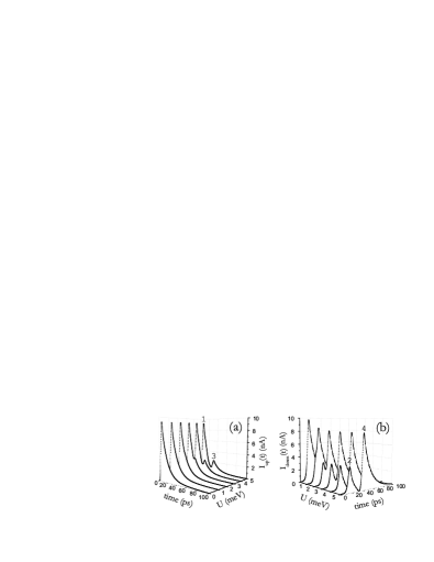
Figure 3: (a) Spin–up and (b) spin–down transient currents in response to a ramp–up voltage for different $U$. Same parameters are adopted as in Fig. 2(b).

Influence of Coulomb interaction on the transient current is illustrated by Fig. 3. Cases of different $U$ ranging from a noninteracting scenario to a strongly blockaded QD are studied. For $U=0$, there is only one peak in $I_{s}(t)$ for either spin, since the excitation energies $\epsilon_{s}$ and $\epsilon_{s}+U$ are indistinguishable. The peak is split into two with an increasing displacement as $U$ is augmented. For either spin direction, the first peak always sticks to its original position as in $U=0$, while the second one emerges later in time with a larger $U$. For $U$ as large as $5\,$meV, the two peaks in $I_{\downarrow}(t)$ are almost completely separated. This confirms our attribution of the peaks to the various resonances: the first peaks in $I_{\uparrow}(t)$ (peak–1) and $I_{\downarrow}(t)$ (peak–2) correspond to the resonances ${\mu}=\epsilon_{\uparrow}$ and ${\mu}=\epsilon_{\downarrow}$, respectively; and the second ones in $I_{\uparrow}(t)$ (peak–3) and $I_{\downarrow}(t)$ (peak–4) are associated with ${\mu}=\epsilon_{\uparrow}+U$ and ${\mu}=\epsilon_{\downarrow}+U$, respectively.

Thermal effect is also explored. $I_{s}(t)$ under different lead temperatures are plotted in Fig. 4. A series of satellite oscillations appears following each resonance peak in $I_{s}(t)$ at a low $T$, which is resulted from a time–varying phase factor, $\exp[\,i\!\int^{t}_{\tau}\!d\bar{t}\,\Delta(\bar{t})]$, of the nonequilibrium lead correlation function. The oscillation frequency is thus determined by the magnitude of $\Delta(t)$. For a ramp–up voltage, $\Delta(t)$ increases monotonically during $0<t<\tau$. It is thus reasonable to find the frequency of satellite oscillations grows with time, and the decaying amplitude of the oscillations is due to the dissipative interactions between the QD and the semi–infinite lead.

To summarize, with a finite switch–on duration $\tau$, the QD energetic configuration is resolved distinctly (sometimes completely) through the resonance peaks of response current in real time, in obvious contrast to the adiabatic charging limit.

Figure 4: Transient current for (a) spin–up and (b) spin–down electrons in response to a ramp–up voltage with $\Delta=10\,$meV, $U=4\,$meV, and $\tau=50\,$ps. The lines represent different temperatures, and separated at $t=0$ by $5\,$nA for clarity. Other parameters are same as in Fig. 2(b).

III.3 The instantaneous switch–on limit

As $\tau$ approaches zero, a ramp–up voltage becomes asymptotically a step pulse, i.e., $\Delta(t)=\Delta\Theta(t)$, with $\Theta(t)$ being the Heaviside step function. Upon the instantaneous switch–on of external voltage, both the spin–up and down QD–levels are activated simultaneously, provided the voltage amplitude $\Delta$ is sufficiently large. It is intriguing to see in this limit how the response current would be related to the QD energetic configuration.

Figure 5: (a) $I_{\uparrow}(t)$ with $\epsilon_{\uparrow}=0$ and (b) $I_{\downarrow}(t)$ with three values of $\epsilon_{\uparrow}$ in unit of meV. Other parameters are (in unit of meV): $\epsilon_{\downarrow}=2.5$, $U=4.5$, $W=5$, $\Gamma=0.05$, $T=0.01$, and $\Delta=10$.

In Fig. 5 (a) and (b) we plot the calculated $I_{\uparrow}(t)$ and $I_{\downarrow}(t)$ in response to a step voltage of $\Delta=10\,$meV, respectively. Three QDs of different $\epsilon_{\uparrow}$ are studied. The energetics scenario for the three QDs are $\mu_{\rm eq}=\epsilon_{\uparrow}<\epsilon_{\downarrow}$, $\mu_{\rm eq}<\epsilon_{\uparrow}<\epsilon_{\downarrow}$, and $\epsilon_{\uparrow}<\mu_{\rm eq}<\epsilon_{\downarrow}$, respectively. Note that for all cases are in a large applied voltage regime since $\Delta>\epsilon_{s}$ and $\Delta>\epsilon_{s}+U$, which ensure all the four QD Fock states accessible energetically. For both spin directions, the transient current shows an initial overshooting, and then oscillates on top of a decay as the reduced system evolves into a steady state with the lead chemical potential $\mu=\Delta$. These rapid oscillations are not artifacts. Their presence reflects the electronic dynamics of QD driven by an external voltage of large amplitude. Upon a small perturbation on $\epsilon_{\uparrow}$ of $0.1\,$meV, $I_{\uparrow}(t)$ scarcely changes as those with $\epsilon_{\uparrow}=\pm\,0.1\,$meV almost overlap with the $\epsilon_{\uparrow}=0$ case shown in Fig. 5(a); while $I_{\downarrow}(t)$ displays drastic deviations among the three cases, in terms of the overshooting amplitude, the oscillation frequency, as well as the decaying rate.

To understand the physical origin of the above observations, frequency–dependent current spectrum is calculated, i.e., $I_{s}(\omega)\equiv\mathcal{F}[I_{s}(t)]$ with $\mathcal{F}$ denoting the conventional Fourier transform. The results corresponding to the three QDs are depicted in Fig. 6. For all three cases, two characteristic frequencies are revealed in $\mbox{Re}[I_{\uparrow}(\omega))]$, i.e., a major kink at $\Delta-\epsilon_{\uparrow}$ and a minor wiggle around $\Delta-\epsilon_{\uparrow}-U$. The line shape of $\mbox{Re\,}[I_{\uparrow}(\omega)]$ around the frequency $\omega_{\uparrow}\equiv\Delta-\epsilon_{\uparrow}$ much resembles that of a single–level QD Zheng08Paper3 . For $\epsilon_{\uparrow}<\mu_{\rm eq}$, $\mbox{Re\,}[I_{\uparrow}(\omega)]$ exhibits a peak at $\omega_{\uparrow}$; while for $\epsilon_{\uparrow}>\mu_{\rm eq}$, a dip shows up. In the case of $\epsilon_{\uparrow}=\mu_{\rm eq}$, $\mbox{Re\,}[I_{\uparrow}(\omega)]$ around $\omega_{\uparrow}$ is described by the function form of $\ln(x^{2}+1)/x$, with $x=2(\omega-\omega_{\uparrow})/\Gamma$. However, the profiles of $\mbox{Re}[I_{\downarrow}(\omega)]$ are significantly different among the three cases. To be specific, for $\epsilon_{\uparrow}=\mu_{\rm eq}$, two prominent dips show up at frequencies $\Delta-\epsilon_{\downarrow}$ and $\Delta-\epsilon_{\downarrow}-U$, respectively; for $\epsilon_{\uparrow}>\mu_{\rm eq}$, the dip at $\Delta-\epsilon_{\downarrow}-U$ is considerably suppressed, which is associated with the transition $\left|\uparrow\right\rangle\leftrightarrow\left|d\right\rangle$; and for $\epsilon_{\uparrow}<\mu_{\rm eq}$, it is the dip at $\Delta-\epsilon$ that is almost completely quenched, which indicates an inactive transition $\left|0\right\rangle\leftrightarrow\left|\downarrow\right\rangle$. Hence it is demonstrated the response current spectrum varies sensitively to the QD energetic configuration.

Figure 6: $\mbox{Re\,}[I_{\uparrow}(\omega)]$ (left panels) and $\mbox{Re\,}[I_{\downarrow}(\omega)]$ (right panels) for three specified values of $\epsilon_{\uparrow}$ (unit of meV) in the top, middle, and bottom panels, respectively, in relation to $\mu_{\rm eq}$. Other parameters are those adopted in Fig. 5, and same for all panels. Insets in (a) and (b) magnify the peaks at $5.5\,$meV and $10\,$meV, respectively.

The presence (or absence) of a resonance signature in $\mbox{Re}[I_{s}(\omega)]$, as well as the issue of peak versus dip at $\omega_{\uparrow}$, are closely related to the equilibrium occupancy of the spin–up state prior to the switch–on of the voltage. Specifically, in the case of $\epsilon_{\uparrow}=0.1\,{\rm meV}\,(>\mu_{\rm eq})$, the initial population of spin–up electrons on the QD is as small as $0.08$, and the subsequent incoming spin–down electrons driven by the step voltage would feel scarcely any Coulomb repulsion due to the almost vacant spin–up level. This thus leads to the prominent dip at $\Delta-\epsilon_{\downarrow}$ and the barely recognizable one at $\Delta-\epsilon_{\downarrow}-U$ in $\mbox{Re}[I_{\downarrow}(\omega)]$; see Fig. 6(b). Whereas in the case of $\epsilon_{\uparrow}=-0.1\,{\rm meV}\,(<\mu_{\rm eq})$, the spin–up level is nearly fully occupied at $t=0$, i.e., $N_{\uparrow}(0)=0.92$. Therefore, the majority of spin–down electrons injected afterwards need to acquire an excess energy of $U$ to overcome the Coulomb blockade, and this is why the dip at $\Delta-\epsilon_{\downarrow}$ becomes trivial; see Fig. 6(f). For $\epsilon_{\uparrow}=\mu_{\rm eq}$, the spin–up level is half occupied ($N_{\uparrow}=0.5$) prior to the switch–on of voltage. In such a circumstance, both the resonant transitions $\left|0\right\rangle\leftrightarrow\left|\downarrow\right\rangle$ and $\left|\uparrow\right\rangle\leftrightarrow\left|d\right\rangle$ contribute equally to the response current, and hence give rise to the two dips of similar depth at frequencies $\Delta-\epsilon_{\downarrow}$ and $\Delta-\epsilon_{\downarrow}-U$; see Fig. 6(d). With $\epsilon_{\uparrow}>0.1\,$meV, the resonance signature in $\mbox{Re}[I_{\uparrow}(\omega)]$ at $\Delta-\epsilon_{\uparrow}$ becomes a pure dip, and the minor dip in $\mbox{Re}[I_{\uparrow}(\omega)]$ at $\Delta-\epsilon_{\downarrow}-U$ vanishes completely; while with $\epsilon_{\uparrow}<-0.1\,$meV, $\mbox{Re}[{I_{\uparrow}(\omega)}]$ shows a pure peak at $\Delta-\epsilon_{\uparrow}$, and the minor dip in $\mbox{Re}[I_{\uparrow}(\omega)]$ at $\Delta-\epsilon_{\downarrow}$ becomes invisible.

This thus confirms that in the instantaneous switch–on limit, the $\omega$–dependent response current spectrum resolves sensitively and faithfully the QD energetic configuration through the characteristic resonance signatures. To our surprise, $\mbox{Re\,}[I_{\downarrow}(\omega)]$ resolves a third peak at $\omega_{\uparrow}$; see the tiny bump in Fig. 6(b) and its inset. It possibly arises due to the higher–order response, and the mechanism of its presence requires further understanding on the transient dynamic processes. At a lower temperature, all the resonance signatures in the current spectrum are accentuated (not shown), i.e., the peaks (dips) become higher (deeper) and sharper. In the real time, this amounts to an enhanced oscillation amplitude of transient current.

IV Concluding remarks

To conclude, we have investigated the transient electronic dynamics of a single–lead interacting QD driven by a family of ramp–up voltages. We have found that (a) in the adiabatic charging limit, the quasi–steady dynamics provide only incomplete information on the QD energetic configuration; (b) With an appropriately chosen switch–on duration, all transitions among QD Fock states can be resolved distinctly through the resonance peaks of transient current in real time, and hence provide comprehensive (sometimes complete) information on the QD energetic configuration; (c) In the instantaneous switch–on limit, the frequency–dependent responses current spectrum reveals sensitively and faithfully the QD energetic configuration through the characteristic resonance signatures. This work thus highlights the significance and versatility of transient dynamics calculations.

In the sequential tunneling regime where $\Gamma\ll T$ (e.g., Figs. 1$-$3), the present HEOM with truncation tier of $N_{\rm trun}=1$, which amounts to the conventional quantum master equation methods with memory Yan05187 , will be sufficient. When $\Gamma\sim T$, calculations with $N_{\rm trun}=1$ would produce qualitatively correct static and dynamic Coulomb blockade for a single–lead QD, because the basic physics does not involve the cotunneling mechanism. However, to obtain quantitatively accurate results, $N_{\rm trun}=2$ is needed. Extensive numerical tests indicate that $N_{\rm trun}=2$ can support up to $\Gamma\sim 5T$ (e.g., Figs. 5 and 6). It has been shown Jin08234703 that the present HEOM theory with $N_{\rm trun}=2$, which properly treats the cotunneling dynamics, is equivalent to a real–time diagrammatic formalism Kon961715 ; thus the Kondo problems can be addressed. However, a higher truncation tier is numerically needed for convergency when $T\ll\Gamma$. The quantitatively accurate results presented in this work (for $\Gamma<5T$) are useful for further development of efficient but maybe approximate computational schemes.

Investigating and/or manipulating transient electronic dynamics provide(s) sometimes a unique way to achieve physical properties and novel functions of mesoscopic many–body systems. However, exact theoretical results for transient quantum transport are rare. Weiss et al Wei08195316 have recently proposed an iterative real–time path integral approach, which is numerically exact but expensive especially when the applied bias voltage is beyond some simple forms such as a step function. The present HEOM theory is formally exact and provides an alternative approach. It is applicable to arbitrary time–dependent external fields applied to leads and/or to the system, without extra computational cost. However, computational effort increases dramatically if the converged results require a high truncation tier of the hierarchy Jin08234703 .

- (1) W. Lu, Z. Ji, L. Pfeiffer, K. W. West, and A. J. Rimberg, Nature 423, 422 (2003).
- (2) J. S. Jin, X. Zheng, and Y. J. Yan, J. Chem. Phys. 128, 234703 (2008).
- (3) R. X. Xu, P. Cui, X. Q. Li, Y. Mo, and Y. J. Yan, J. Chem. Phys. 122, 041103 (2005).
- (4) R. X. Xu and Y. J. Yan, Phys. Rev. E 75, 031107 (2007).
- (5) J. S. Jin et al., J. Chem. Phys. 126, 134113 (2007).
- (6) R. P. Feynman and F. L. Vernon, Jr., Ann. Phys. (N. Y.) 24, 118 (1963).
- (7) Y. Tanimura, Phys. Rev. A 41, 6676 (1990).
- (8) C. Meier and D. J. Tannor, J. Chem. Phys. 111, 3365 (1999).
- (9) Y. J. Yan and R. X. Xu, Annu. Rev. Phys. Chem. 56, 187 (2005).
- (10) M. L. Polianski, P. Samuelsson, and M. Büttiker, Phys. Rev. B 72, 161302 (2005).
- (11) M. L. Polianski and M. Büttiker, Phys. Rev. B 76, 205308 (2007).
- (12) J. Fransson, Int. J. Quant. Chem 92, 471 (2003).
- (13) M. H. Pedersen and M. Büttiker, Phys. Rev. B 58, 12993 (1998).
- (14) P. W. Anderson, Phys. Rev. 124, 41 (1961).
- (15) W. H. Press, S. A. Teukolsky, W. T. Vetterling, and B. P. Flannery, Numerical Recipes in Fortran, Cambridge University Press, New York, 1992.
- (16) R. Baer and D. Neuhauser, J. Chem. Phys. 121, 9803 (2004).
- (17) F. Wang, C.-Y. Yam, G. H. Chen, and K. N. Fan, J. Chem. Phys. 126, 134104 (2007).
- (18) X. Zheng, J. S. Jin, and Y. J. Yan, Phys. Rev. B (2008).
- (19) J. König, H. Schoeller, and G. Schön, Phys. Rev. Lett. 76, 1715 (1996).
- (20) S. Weiss, J. Eckel, M. Thorwart, and R. Egger, Phys. Rev. B 77, 195316 (2008).