Preterm Birth Analysis Using Nonlinear Methods
(a preliminary study)

Abstract

In this report we review modern nonlinearity methods that can be used in the preterm birth analysis. The nonlinear analysis of uterine contraction signals can provide information regarding physiological changes during the menstrual cycle and pregnancy. This information can be used both for the preterm birth prediction and the preterm labor control.

Keywords: preterm birth, complex data analysis, nonlinear methods

1 Introduction

Preterm birth is the single most important cause of perinatal mortality in North America and Europe [Berkowitz & Papiernik, 1993]. Developed countries represent 20 % of the population in the world, but only 12 % of human births annually, while 98 % of medical publications are issued from these areas. Reproductive patterns in the developed world, for the last three decades, are different from elsewhere and during the first 70 years of the 20th century. A major difference is in the number of children in families but also, and mainly, in the ages at first pregnancies in primiparae (approaching now 30 years in many developed countries) [Robillard et al., 2007]. A British study [Rush et al., 1976] has estimated that preterm birth accounts for 85 percent of early neonatal deaths that are not caused by lethal congenital malformations. In the United States, the smallest of the preterm infants those weighing less than 750 g have been found to account for 41 percent of early neonatal deaths and 25 percent of infant deaths [Overpeck et al., 1992]. Preterm birth is also a major determinant of neonatal and infant morbidity, including neuro-developmental handicaps, chronic respiratory problems, intraventricular hemorrhage, infection, retrolental fibroplasia, and necrotizing enterocolitis [Nat. Acad. Sci, 1985, Arias & Tomich, 1993]. While there are inconsistent results with regard to long-term somatic growth among preterm infants [Kitchen et al., 1992, Ross et al., 1990], the risk of neurologic and developmental impairment during childhood is substantially elevated for the smallest survivors [Escobar et al., 1991, Veen et al., 1991]. In addition, the neonatal and long-term health care costs of preterm infants impose a considerable economic burden both on individual families and nationally [Nat. Acad. Sci, 1985].

While the frequency of births of low birth weight (less then 2,500 g) infants declined somewhat in the United States between 1970 and 1980, this decline appears to have occurred primarily among full-term as opposed to preterm low birth weight infants [Kessel et al., 1984]. Furthermore, although the infant mortality rate has decreased substantially since 1965, improvement in infant survival has been attributed principally to reduced birth weight-specific mortality rather than to changes in the birth weight or gestational age distribution [Kleinman & Kessel, 1981]. Despite the reduction in infant mortality, the rate in the United States remains considerably higher than the rates in many other industrialized countries. It is unlikely that there will be further substantial improvement in infant survival in the United States unless a reduction in births of preterm low birth weight infants can be accomplished [Berkowitz & Papiernik, 1993].

Traditionally, prematurity was defined as a birth weight less than or equal to 2,500 g. However, studies performed during the 1960s and 1970s revealed that this definition encompasses three distinct types of infants: those who are small because they were born too early, those who are small because their growth was retarded in utero, and those who are small because they were both premature and growth-retarded. The label prematurity has now been replaced by the terms low birth weight and preterm. According to current World Health Organization nomenclature [World Health Org. 1977], low birth weight characterizes an infant who weighs less than 2,500 g (5 pounds and 8 ounces) at birth, and preterm refers to a birth that occurs at a gestational age of less than 37 completed weeks (less then 259 days).

A cutoff of 37 weeks for defining preterm birth, albeit arbitrary, is now well established, but some studies have used cutoffs of 36 or 38 weeks of gestation. In addition, some investigators have only included preterm infants of a particular weight, such as those weighing less than 2,500 g. Further subdivisions have also been used in the recent literature, such as very low birth weight to describe an infant weighing less than 1,500 g or 1,000 g at birth, and very preterm for gestational ages variously defined as less than 32, 33, or 34 weeks. Use of these lower cutoffs should be encouraged, since it will permit identification of risk factors that have the greatest impact on neonatal mortality [Berkowitz & Papiernik, 1993].

For detecting contractions in uterine electromyography (EMG), fast numerical algorithms have been developed [Radharkrishnan et al., 2000]. Recently, the analysis of uterine contraction signals has provided information regarding physiological changes during the menstrual cycle and pregnancy [Oczeretko et al., 2006]. The authors have presented the cross-correlation and the wavelet cross-correlation methods to assess synchronization between contractions in different topographic regions of the uterus. It is important to identify time delays between uterine contractions, which may be of potential diagnostic significance in various pathologies. The cross-correlation was computed in a moving window with a width corresponding to approximately two or three contractions. As a result, the running cross-correlation function was obtained. The propagation % parameter assessed from this function allows quantitative description of synchronization in bivariate time series. In general, the uterine contraction signals are very complicated. Wavelet transforms provide insight into the structure of the time series at various frequencies (scales). To show the changes of the propagation % parameter along scales, a wavelet running cross-correlation was used. At first, the continuous wavelet transforms as the uterine contraction signals were received and afterwards, a running cross-correlation analysis was conducted for each pair of transformed time series. The findings of [Oczeretko et al., 2006] show that running functions are very useful in the analysis of uterine contractions.

Fractal analysis serves another example for advanced data analysis to be utilized in the studies on uterine contractile activity. Fractals, a relatively new analytical concept of the last few decades, have been successfully applied in many areas of science and technology. [Oczeretko et al., 2004] performed a comparative study of ten methods of fractal analysis of signals of intrauterine pressure, and found significant differences between uterine contractions in healthy volunteers and women with primary dysmenorrhoea. There was a correlation between the adjacent elements of the investigated signals. Consequently, the values of fractal dimension can be objective measures for classifications of uterine contraction signals and may be used in studies on preterm labor.

Nonlinear dynamics is one more example of advanced data analysis that could be implemented for uterine contractility signals [Pierzynski et al., 2007]. In recent years the physiological signals obtained from the complex systems like the brain or the heart have been investigated for possible deterministic chaotic behavior. The human uterus is undoubtedly a complex system. Smooth muscles comprising the myometrium interact in a complex manner. The techniques of surrogate data analysis have been used to testing for nonlinearity in the uterine contraction signals. The results showed that the spontaneous uterine contractions are considered to contain nonlinear features [Oczeretko et al., 2005] which indicated that nonlinear dynamics may increase the accessibility of data for the assessment of biology of uterus, and consequently, the nature of preterm labor.

2 Techniques of Nonlinear Dynamics and Complex Data Analysis

In this section we review the concept of nonlinearity (as contrasted with the standard textbook linear algebra, analysis, statistics, etc.), together with its geometrical picture, and its extreme dynamics of chaotic behavior.

2.1 Nonlinear Dynamics

Recall that nonlinear dynamics is a modern language to talk about dynamical systems. It is a general theory of systems arising in physics, engineering, chemistry, biology, psychology, sociology and economics. Nonlinear dynamics has two extremes: at one end it is classical linear dynamics, fully predictable and controllable, as usually explained in engineering textbooks. On the other end, it is chaotic dynamics, or popularly, the “chaos theory.” Nonlinear dynamics includes both of these extremes, as well as all other natural and artificial dynamics. Its main keywords are (see, e.g., [Ivancevic & Ivancevic, 2006a]):

• Dynamical system: A part of the world which can be seen as a self–contained entity with some temporal behavior. In nonlinear dynamics, speaking about a dynamical system usually means to speak about an abstract mathematical system which is a model for such an entity. Mathematically, a dynamical system is defined by its state and by its dynamics. A pendulum is an example for a dynamical system.

• State of a system: A number or a vector (i.e., a list of numbers) defining the state of the dynamical system uniquely. For the free (un–driven) pendulum, the state is uniquely defined by the angle $\theta$ and the angular velocity $\dot{\theta}=d\theta/dt$. In the case of driving, the driving phase $\phi$ is also needed because the pendulum becomes a non–autonomous system. In spatially extended systems, the state is often a field (a scalar–field or a vector–field). Mathematically spoken, fields are functions with space coordinates as independent variables. The velocity vector–field of a fluid is a well–known example.

• Phase space: All possible states of the system. Each point in the phase–space corresponds to a unique state. In the case of the free pendulum, the phase–space has 2D whereas for driven pendulum it has 3D. The dimension of the phase–space is infinite in cases where the system state is defined by a field.

• Dynamics, or equation of motion: The causal relation between the present state and the next state in the future. It is a deterministic rule which tells us what happens in the next time step. In the case of a continuous time, the time step is infinitesimally small. Thus, the equation of motion is an ordinary differential equation (ODE) (or a system of ODEs):

  $$\dot{x}=f(x),$$

  where $x$ is the state and $t$ is the time variable (overdot is the time derivative – as always). An example is the equation of motion of an un–driven and un–damped pendulum. In the case of a discrete time, the time steps are nonzero and the dynamics is a map:

  $$x_{n+1}=f(x_{n}),$$

  with the discrete time $n$. Note, that the corresponding physical time points $t_{n}$ do not necessarily occur equidistantly. Only the order has to be the same. That is,

  $$n<m\qquad\Longrightarrow\qquad t_{n}<t_{m}.$$

  The dynamics is linear if the causal relation between the present state and the next state is linear. Otherwise it is nonlinear. If we have the case in which the next state is not uniquely defined by the present one, this is generally an indication that the phase–space is not complete. Thus, there are important variables determining the state which had been forgotten. This is a crucial point while modelling a real–life systems. Beside this, there are two important classes of systems where the phase–space is incomplete: the non–autonomuous and stochastic systems. A non–autonomous system has an equation of motion which depends explicitly on time. Thus, the dynamical rule governing the next state not only depends on the present state but also at the time it applies. A driven pendulum is a classical example of a non–autonomuous system. Fortunately, there is an easy way to make the phase–space complete: we simply include the time into the definition of the state. Mathematically, this is done by introducing a new state variable: $t$. Its dynamics reads

  $$\dot{t}=1,\qquad\text{or}\qquad t_{n+1}=t_{n},$$

  depending on whether time is continuous or discrete. For the periodically driven pendula, it is also natural to take the driving phase as the new state variable. Its equation of motion reads

  $$\dot{\theta}=2\pi w,$$

  where $w$ is the driving frequency (so that the angular driving frequency is $2\pi w$). On the other hand, in a stochastic system, the number and the nature of the variables necessary to complete the phase–space is usually unknown. Therefore, the next state can not be deduced from the present one. The deterministic rule is replaced by a stochastic one. Instead of the next state, it gives only the probabilities of all points in the phase–space to be the next state.

• Orbit or trajectory: A solution of the equation of motion. In the case of continuous time, it is a curve in phase–space parameterized by the time variable. For a discrete system it is an ordered set of points in the phase–space.

• Phase Flow: The mapping (or, map) of the whole phase–space of a continuous dynamical system onto itself for a given time step $t$. If $t$ is an infinitesimal time step $dt$, the flow is just given by the right–hand side of the equation of motion (i.e., $f$). In general, the flow for a finite time step is not known analytically because this would be equivalent to have a solution of the equation of motion.

More precisely, a mathematical term dynamical system geometrically represents a vector–field in the system’s phase–space manifold $M$ (see [Ivancevic & Ivancevic, 2006b]), which upon integration (governed by the celebrated existence & uniqueness theorems for ordinary Differential Equations) defines a phase–flow in $M$ (see Figure 1). This phase–flow $f_{t}\in M$, describing the complete behavior of a dynamical system at every time instant, can be either linear, nonlinear or chaotic.

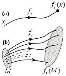
Figure 1: Action of the phase–flow $f_{t}$ in the phase–space manifold $M$: (a) Trajectory of a single initial point $x(t)\in M$ , (b) Transporting the whole manifold $M$ (see [Ivancevic & Ivancevic, 2006a]).

Before the advent of fast computers, solving a dynamical system required sophisticated mathematical techniques and could only be accomplished for a small class of linear dynamical systems. Numerical methods executed on computers have simplified the task of determining the orbits of a dynamical system.

For simple dynamical systems, knowing the trajectory is often sufficient, but most dynamical systems are too complicated to be understood in terms of individual trajectories. The difficulties arise because:

1. The systems studied may only be known approximately–the parameters of the system may not be known precisely or terms may be missing from the equations. The approximations used bring into question the validity or relevance of numerical solutions. To address these questions several notions of stability have been introduced in the study of dynamical systems, such as Lyapunov stability or structural stability. The stability of the dynamical system implies that there is a class of models or initial conditions for which the trajectories would be equivalent. The operation for comparing orbits to establish their equivalence changes with the different notions of stability.

2. The type of trajectory may be more important than one particular trajectory. Some trajectories may be periodic, whereas others may wander through many different states of the system. Applications often require enumerating these classes or maintaining the system within one class. Classifying all possible trajectories has led to the qualitative study of dynamical systems, that is, properties that do not change under coordinate changes. Linear dynamical systems and systems that have two numbers describing a state are examples of dynamical systems where the possible classes of orbits are understood.

3. The behavior of trajectories as a function of a parameter may be what is needed for an application. As a parameter is varied, the dynamical systems may have bifurcation points where the qualitative behavior of the dynamical system changes. For example, it may go from having only periodic motions to apparently erratic behavior, as in the transition to turbulence of a fluid.

4. The trajectories of the system may appear erratic, as if random. In these cases it may be necessary to compute averages using one very long trajectory or many different trajectories. The averages are well defined for ergodic systems and a more detailed understanding has been worked out for hyperbolic systems. Understanding the probabilistic aspects of dynamical systems has helped establish the foundations of statistical mechanics and of chaos.

2.2 Geometrical View on Nonlinear Dynamics

Geometrically speaking (see [Ivancevic & Ivancevic, 2006b]), linear systems (i.e., systems defined by linear differential equations) live in Euclidean spaces $\mathbb{R}^{N}$, where $N$ is the dimension of the system. For their analysis the tools of linear algebra and calculus are used. The basic measure here is the global Euclidean metric form (or, Euclidean distance function) function on the system coordinates, defined by

$$S=\sqrt{\sum_{i=1}^{N}\left(x_{i}-y_{i}\right)^{2}},\qquad\text{or\qquad}S^{2}=\sum_{i=1}^{N}\left(x_{i}-y_{i}\right)^{2}.$$

The more realistic nonlinear systems (i.e., systems defined by non-linear differential equations) can be considered as local deformations of the closest linear systems and they live in smooth manifolds ${M}^{N}.$ For their analysis the tools of Riemannian geometry are used, with the local Riemannian metric form, defined by

$$ds^{2}=\sum_{i=1}^{N}\sum_{j=1}^{N}g_{ij}dx_{i}dx_{j},\qquad\text{or\qquad}ds^{2}=g_{ij}dx^{i}dx^{j},$$ (1)

where $g_{ij}$ is the Riemannian metric tensor, $dx^{i}$ are differentials of the local coordinates, and the Einstein’s summation convention (summing upon repeated indices if one is superscript-contravariant and the other is subscript-covariant) is in place. Besides giving the local distances between the points on the smooth manifold $\mathbb{M}^{N},$ the Riemannian metric form (1) defines the system’s kinetic energy

$$KE=\frac{1}{2}g_{ij}\dot{x}^{i}\dot{x}^{j},\qquad(\text{overdot means time derivative}),$$

giving the Euler-Lagrangian equations of motion in a geometrical form (for $s=t$) of geodesic equations

$$\frac{d^{2}x^{i}}{ds^{2}}+\Gamma_{jk}^{i}\frac{dx^{j}}{ds}\frac{dx^{k}}{ds}=0,$$ (2)

where $\Gamma_{jk}^{i}$ are the so–called Christoffel symbols of the affine Levi-Civita connection of the manifold ${M}^{N}$ (see, e.g., [Ivancevic & Ivancevic, 2007b]).

In the geometrical framework, the (in)stability of the trajectories is the (in)stability of the geodesics, and it is completely determined by the curvature properties of the underlying manifold according to the Jacobi equation of geodesic deviation
[Ivancevic & Ivancevic, 2007b]

$$\frac{D^{2}J^{i}}{ds^{2}}+R_{~{}jkm}^{i}\frac{dx^{j}}{ds}J^{k}\frac{dx^{m}}{ds}=0,$$ (3)

whose solution $J$, usually called Jacobi variation field, locally measures the distance between nearby geodesics; $D/ds$ stands for the covariant derivative along a geodesic and $R_{~{}jkm}^{i}$ are the components of the Riemann curvature tensor.

In the special case of the Eisenhart metric [Eisenhart, 1929] on an enlarged configuration space–time ($\{x^{0}\equiv t,x^{1},\ldots,x^{N}\}$, the Jacobi equation (3) reduces to the tangent dynamics equation [Ivancevic & Ivancevic, 2007b]

$$\frac{d^{2}J^{i}}{dt^{2}}+\left(\frac{\partial^{2}V}{\partial x^{i}\partial x^{k}}\right)_{x(t)}J^{k}=0.$$ (4)

2.3 Extreme Nonlinearity: Chaotic Dynamics

On the other hand, chaotic dynamics, the most extreme case of nonlinear dynamics, is highly sensitive to both initial conditions (popularly referred to as the butterfly effect) and system parameters. As a result of this sensitivity, which manifests itself as an exponential growth of perturbations in the initial conditions, the behavior of chaotic systems appears to be random. This happens even though these systems are deterministic, meaning that their future dynamics are fully defined by their initial conditions, with no random elements involved. This behavior is known as deterministic chaos (see, e.g., [Ivancevic & Ivancevic, 2006a]). Chaotic behavior has been observed in the laboratory in a variety of systems including electrical circuits, lasers, oscillating chemical reactions, fluid dynamics, and mechanical and magneto-mechanical devices.

Chaotic behavior is surprisingly complex and may arise in a simple noise-free system with few degrees of freedom. Chaos is globally stable and locally unstable. A chaotic system neither reaches a certain steady state nor repeats itself periodically. Thus, it is a pure disordered process since no points or patterns of points ever recur. However, its activity remains constrained within a certain boundary, which may suggest a new kind of order. Chaotic behavior resembles random noise, but is predictable in the short-term. This short-term predictability is useful in various domains ranging from weather forecasting to economic forecasting [Hilborn, 1994].

The most common route to chaos is a sequence of period-doubling bifurcations, caused by particular values of a nonlinear system parameter. The cases of most interest arise when the chaotic behavior takes place on an attractor, since then a large set of initial conditions will lead to orbits that converge to this chaotic region. In particular, the so–called strange attractors typically have a fractal structure. In all chaotic systems all particle trajectories diverge exponentially from one another, with a positive Lyapunov exponent. Besides, chaotic behavior is related to the non-equilibrium phase transitions caused by system’s topology change [Caiani et al., 1997, Franzosi et al., 1999, Franzosi et al., 2000].

Techniques have emerged to harness chaos to the benefit of humans. The chaotic behavior of a system may be artificially weakened or suppressed if it is undesirable. This concept is known as control of chaos. The first and the most important method of chaos control is the so–called OGY–method, developed by [Ott et al., 1990]. However, in recent years, a non-traditional concept of anti-control of chaos has emerged. Here, the non-chaotic dynamical system is transformed into a chaotic one by small controlled perturbation so that useful properties of a chaotic system can be exploited. This non-traditional concept has found applications in time and energy critical control applications such as navigation in a multi-body planetary system, fluid mixing and to secure information processing [Chen & Dong, 1998].

2.3.1 Lorenz Attractor

Recall that a dynamical system may be defined as a deterministic rule for the time evolution of state observables. Well known examples are ODEs in which time is continuous [Ivancevic & Ivancevic, 2006a]

$$\mathbf{\dot{x}}(t)=\mathbf{f}(\mathbf{x}(t)),\;\;\;\;\;(\mathbf{x},\mathbf{f}\in\mathbb{R}^{n});$$ (5)

and iterative maps in which time is discrete:

$$\mathbf{x}(t+1)=\mathbf{g}(\mathbf{x}(t)),\;\;\;\;\;(\mathbf{x},\mathbf{g}\in\mathbb{R}^{n}).$$ (6)

In the case of maps, the evolution law is straightforward: from $\mathbf{x}(0)$ one computes $\mathbf{x}(1)$, and then $\mathbf{x}(2)$ and so on. For ODE’s, under rather general assumptions on $\mathbf{f}$, from an initial condition $\mathbf{x}(0)$ one has a unique trajectory $\mathbf{x}(t)$ for $t>0$ [Ott, 1993]. Examples of regular behaviors (e.g., stable fixed–points, limit cycles) are well known, see Figure 2.

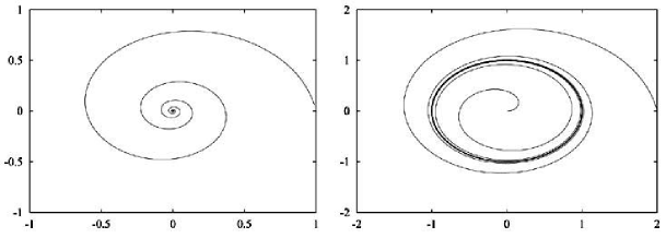
Figure 2: Examples of regular attractors: fixed–point (left) and limit cycle (right). Note that limit cycles exist only in nonlinear dynamics.

A rather natural question is the possible existence of less regular behaviors i.e., different from stable fixed–points, periodic or quasi-periodic motion.

After the seminal works of Poincaré, Lorenz, Smale, May, and Hénon (to cite only the most eminent ones) it is now well established that the so called chaotic behavior is ubiquitous. As a relevant system, originated in the geophysical context, we mention the celebrated Lorenz system [Lorenz, 1963, Sparrow, 1982]

$$\dot{x} = -\sigma(x-y)$$

$$\dot{y} = -xz+rx-y$$ (7)

$$\dot{z} = xy-bz$$

This system is related to the Rayleigh–Bénard convection under very crude approximations. The quantity $x$ is proportional the circulatory fluid particle velocity; the quantities $y$ and $z$ are related to the temperature profile; $\sigma$, $b$ and $r$ are dimensionless parameters. Lorenz studied the case with $\sigma=10$ and $b=8/3$ at varying $r$ (which is proportional to the Rayleigh number). It is easy to see by linear analysis that the fixed–point $(0,0,0)$ is stable for $r<1$. For $r>1$ it becomes unstable and two new fixed–points appear

$$C_{+,-}=(\pm\sqrt{b(r-1)},\pm\sqrt{b(r-1)},r-1),$$ (8)

these are stable for $r<r_{c}=24.74$. A nontrivial behavior, i.e., non periodic, is present for $r>r_{c}$, as is shown in Figure 3.

In this ‘strange’, chaotic regime one has the so called sensitive dependence on initial conditions. Consider two trajectories, $\mathbf{x}(t)$ and $\mathbf{x}^{\prime}(t)$, initially very close and denote with $\Delta(t)=||\mathbf{x}^{\prime}(t)-\mathbf{x}(t)||$ their separation. Chaotic behavior means that if $\Delta(0)\to 0$, then as $t\to\infty$ one has $\Delta(t)\sim\Delta(0)\exp{\lambda_{1}t}$, with $\lambda_{1}>0$ [Boffetta et al., 2001].

Let us notice that, because of its chaotic behavior and its dissipative nature, i.e.,

$${\frac{\partial\dot{x}}{\partial x}}+{\frac{\partial\dot{y}}{\partial y}}+{\frac{\partial\dot{z}}{\partial z}}<0,$$ (9)

the attractor of the Lorenz system cannot be a smooth surface. Indeed the attractor has a self–similar structure with a fractal dimension between $2$ and $3$. The Lorenz model (which had an important historical relevance in the development of chaos theory) is now considered a paradigmatic example of a chaotic system.

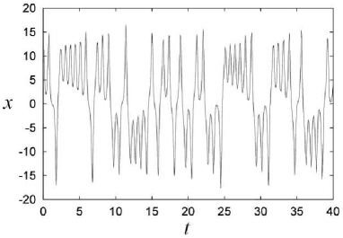
Figure 3: Example of an aperiodic signal: the $x$ variable of the Lorenz system (7) as function of time $t$, for $r=28$.

2.3.2 Lyapunov Exponents

The sensitive dependence on the initial conditions can be formalized in order to give it a quantitative characterization. The main growth rate of trajectory separation is measured by the first (or maximum) Lyapunov exponent, defined as (see, e.g., [Boffetta et al., 2001])

$$\lambda_{1}=\lim_{t\rightarrow\infty}\lim_{\Delta(0)\rightarrow 0}{\frac{1}{t}}\ln{\frac{\Delta(t)}{\Delta(0)}},$$ (10)

As long as $\Delta(t)$ remains sufficiently small (i.e., infinitesimal, strictly speaking), one can regard the separation as a tangent vector $\mathbf{z}(t)$ whose time evolution is

$$\dot{z}_{i}={\frac{\partial f_{i}}{\partial x_{j}}}|_{\mathbf{x}(t)}\cdot z_{j},$$ (11)

and, therefore,

$$\lambda_{1}=\lim_{t\rightarrow\infty}{\frac{1}{t}}\ln{\frac{||\mathbf{z}(t)||}{||\mathbf{z}(0)||}}.$$ (12)

In principle, $\lambda_{1}$ may depend on the initial condition $\mathbf{x}(0)$, but this dependence disappears for ergodic systems. In general there exist as many Lyapunov exponents, conventionally written in decreasing order $\lambda_{1}\geq\lambda_{2}\geq\lambda_{3}\geq...$, as the independent coordinates of the phase–space [Benettin et al., 1980]. Without entering the details, one can define the sum of the first $k$ Lyapunov exponents as the growth rate of an infinitesimal $k$D volume in the phase–space. In particular, $\lambda_{1}$ is the growth rate of material lines, $\lambda_{1}+\lambda_{2}$ is the growth rate of $2D$ surfaces, and so on. A numerical widely used efficient method is due to [Benettin et al., 1980].

It must be observed that, after a transient, the growth rate of any generic small perturbation (i.e., distance between two initially close trajectories) is measured by the first (maximum) Lyapunov exponent $\lambda_{1}$, and $\lambda_{1}>0$ means chaos. In such a case, the state of the system is unpredictable on long times. Indeed, if we want to predict the state with a certain tolerance $\Delta$ then our forecast cannot be pushed over a certain time interval $T_{P}$, called predictability time, given by [Boffetta et al., 2001]:

$$T_{P}\sim{\frac{1}{\lambda_{1}}}\ln{\frac{\Delta}{\Delta(0)}}.$$ (13)

The above relation shows that $T_{P}$ is basically determined by $1/\lambda_{1}$, seen its weak dependence on the ratio $\Delta/\Delta(0)$. To be precise one must state that, for a series of reasons, relation (13) is too simple to be of actual relevance [Boffetta et al., 2002].

2.3.3 Kolmogorov–Sinai Entropy

Deterministic chaotic systems, because of their irregular behavior, have many aspects in common with stochastic processes. The idea of using stochastic processes to mimic chaotic behavior, therefore, is rather natural [Chirikov, 1979, Benettin, 1984]. One of the most relevant and successful approaches is symbolic dynamics [Beck & Schlögl, 1993]. For the sake of simplicity let us consider a discrete time dynamical system. One can introduce a partition $\mathcal{A}$ of the phase–space formed by $N$ disjoint sets $A_{1},...,A_{N}$. From any initial condition one has a trajectory

$$\mathbf{x}(0)\rightarrow\mathbf{x}(1),\mathbf{x}(2),...,\mathbf{x}(n),...$$ (14)

dependently on the partition element visited, the trajectory (14), is associated to a symbolic sequence

$$\mathbf{x}(0)\rightarrow i_{1},i_{2},...,i_{n},...$$ (15)

where $i_{n}$ ($n=1,2,...,N$) means that $\mathbf{x}(n)\in A_{i_{n}}$ at the step $n$, for $n=1,2,...$. The coarse-grained properties of chaotic trajectories are therefore studied through the discrete time process (15).

An important characterization of symbolic dynamics is given by the Kolmogorov–Sinai entropy (KS), defined as follows. Let $C_{n}=(i_{1},i_{2},...,i_{n})$ be a generic ‘word’ of size $n$ and $P(C_{n})$ its occurrence probability, the quantity [Boffetta et al., 2001]

$$H_{n}=\sup_{A}[-\sum_{C_{n}}P(C_{n})\ln P(C_{n})],$$ (16)

is called block entropy of the $n-$sequences, and it is computed by taking the largest value over all possible partitions. In the limit of infinitely long sequences, the asymptotic entropy increment

$$h_{KS}=\lim_{n\rightarrow\infty}H_{n+1}-H_{n},$$ (17)

is the Kolmogorov–Sinai entropy. The difference $H_{n+1}-H_{n}$ has the intuitive meaning of average information gain supplied by the $(n+1)-$th symbol, provided that the previous $n$ symbols are known. KS–entropy has an important connection with the positive Lyapunov exponents of the system [Ott, 1993]:

$$h_{KS}=\sum_{\lambda_{i}>0}\lambda_{i}.$$ (18)

In particular, for low–dimensional chaotic systems for which only one Lyapunov exponent is positive, one has $h_{KS}=\lambda_{1}$.

We observe that in (16) there is a technical difficulty, i.e., taking the sup over all the possible partitions. However, sometimes there exits a special partition, called generating partition, for which one finds that $H_{n}$ coincides with its superior bound. Unfortunately the generating partition is often hard to find, even admitting that it exist. Nevertheless, given a certain partition, chosen by physical intuition, the statistical properties of the related symbol sequences can give information on the dynamical system beneath. For example, if the probability of observing a symbol (state) depends only by the knowledge of the immediately preceding symbol, the symbolic process becomes a Markov chain (see [Ivancevic & Ivancevic, 2006b]) and all the statistical properties are determined by the transition matrix elements $W_{ij}$ giving the probability of observing a transition $i\rightarrow j$ in one time step. If the memory of the system extends far beyond the time step between two consecutive symbols, and the occurrence probability of a symbol depends on $k$ preceding steps, the process is called Markov process of order $k$ and, in principle, a $k$ rank tensor would be required to describe the dynamical system with good accuracy. It is possible to demonstrate that if $H_{n+1}-H_{n}=h_{KS}$ for $n\geq k+1$, $k$ is the (minimum) order of the required Markov process. It has to be pointed out, however, that to know the order of the suitable Markov process we need is of no practical utility if $k\gg 1$.

2.4 Nonlinear Analysis of Time Series Data

In this subsection, following [Sharma, 2006], we apply two basic techniques of nonlinear dynamics to the heart inter-beat interval (IBI) time series data. The volunteer participant was a twenty year-old male pilot with 400 hours total flight experience and a commercial pilot license. He flew a single-engine aircraft in a fixed-base generic flight simulator. A Polar Heart-rate Receiver/Transmitter was used to record his heart IBI. The task of the participant in the flight segments M1 and M2 was to maintain manually a set airspeed, altitude, and heading as closely as possible. The only difference between the two segments, M1 and M2, was the level of perceived risk of mid-air collision involved if the participant was unable to execute the task adequately. First, a sample participant’s heart IBI data at segments M1 and M2 are represented graphically and analyzed in terms of phase plots. Next, the measure of approximate entropy is employed to quantify the dynamics for each time series [Sharma, 2006].

2.4.1 Phase Plots

The qualitative dynamics of a system may be represented in a graphical form. The Phase plot is the simplest graphical representation of the temporal information contained in a time series. It relates the current value of the time series to its preceding value. However, the preceding value is expressed in such a manner that it is approximately equal to the derivative of the current value. The phase plot provides a spatial representation of the evolving dynamics of a nonlinear system, giving some information on how the process evolves over time [Williams, 1997].

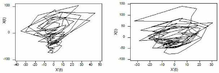
Figure 4: Two-dimensional phase plots of heart inter-beat interval (IBI) for a pilot at the simulated flying segments M1 (left) and M2 (right; adapted from [Sharma, 2006]).

Figure 4 represents two-dimensional phase plots employed to depict the graphical dynamics of a sample participant’s heart IBI at flight segments M1 and M2. The figure shows that the two plots are qualitatively different from each other in terms of their dynamics within the manifold, which is represented by their trajectories. This suggests that they have different vector fields that govern their evolution within their manifolds. Further, a thorough analysis indicates that the system entropy (information content) at segment M2 is slightly higher than that at segment M1. In other words, the heart IBI dynamics at segment M2 appears slightly less structured compared to that at segment M1. However, some quantitative evidence may be required to support this observation, which has been done in the next section. The above observations suggest that heart IBI dynamics depends on the level of the pilot’s perceived risk [Sharma, 2006].

2.4.2 Approximate Entropy

In general, entropy is concerned with information about the state of a dynamical system. Approximate entropy ($ApEn$) is a useful general measure of nonlinear dynamics. The technical details of the $ApEn$ index have been provided in [Pincus, 1995]. $ApEn$ is a measure quantifying the regularity of the time series [Pikkujamsa et al., 1999]. $ApEn$ is defined as

$$ApEn\left({m,r}\right)={\mathop{\lim}\limits_{N\to\infty}}{\left[{\phi\left({m,r,N}\right)-\phi\left({m+1,r,N}\right)}\right]}$$

where $m$ is the maximum run length, $r$ is the tolerance, $N$ is the total number of observations in the time series, and $\phi\left({m,r,N}\right)$ is the average value of the logarithm of proportion of vectors that are closer than the $r$over all vectors. $ApEn$ has a relatively lower value for a structured/deterministic data set and a higher value for a disordered/less-deterministic data set [Ho et al., 1997].

An algorithm has been provided in [Kaplan et al., 1991] to compute $ApEn$. The algorithm detects similar patterns in a time series and then estimates the logarithmic likelihood that the following observation will differ from the previously observed pattern. Further, the pattern length and the pattern similarity criterion can be manipulated while running the program [Ho et al., 1997]. $ApEn$ can be computed using no more than 100 observations [Pincus, 1995].

[Sharma, 2006] employed $ApEn$ to analyze the heart IBI dynamics of a pilot during flight segments M1 and M2. During the analysis, the value for the maximum run length ($m$) was set equal to 2 and the tolerance ($r$) was selected as 0.15 of the standard deviation as suggested in [Pincus, 1995]. The resulting $ApEn$ values at segments M1 and M2 were 0.452 and 0.551 respectively. These quantitative results indicate that the heart IBI $ApEn$ becomes higher at segment M2 compared to that at segment M1. These results re-confirm the visual analysis of the heart IBI Phase Plot data in the previous section, where the entropy at segment M2 was believed to be slightly higher than that at segment M1. This result may further imply that the structure of the heart IBI data becomes more disordered and unstructured during a higher level of perceived-risk. Finally, these results suggest that the heart IBI $ApEn$ may be a sensitive index of the level of perceived risk.

2.5 Lyapunov Exponents in Time Series Data

Recall that chaos arises from the exponential growth of infinitesimal perturbations, together with global folding mechanisms to guarantee boundedness of the solutions. This exponential instability is characterized by the spectrum of Lyapunov exponents
[Eckmann & Ruelle, 1985]. If one assumes a local decomposition of the phase space into directions with different stretching or contraction rates, then the spectrum of exponents is the proper average of these local rates over the whole invariant set, and thus consists of as many exponents as there are space directions. The most prominent problem in time series analysis is that the physical phase space is unknown, and that instead the spectrum is computed in some embedding space. Thus the number of exponents depends on the reconstruction, and might be larger than in the physical phase space. Such additional exponents are called spurious, and there are several suggestions to either avoid them, or to identify them. Moreover, it is plausible that only as many exponents can be determined from a time series as are entering the Kaplan Yorke formula (see below). To give a simple example: Consider motion of a high-dimensional system on a stable limit cycle. The data cannot contain any information about the stability of this orbit against perturbations, as long as they are exactly on the limit cycle. For transients, the situation can be different, but then data are not distributed according to an invariant measure and the numerical values are thus difficult to interpret. Apart from these difficulties, there is one relevant positive feature: Lyapunov exponents are invariant under smooth transformations and are thus independent of the measurement function or the embedding procedure. They carry a dimension of an inverse time and have to be normalized to the sampling interval [Hegger et al., 1999].

2.5.1 The Maximal Lyapunov Exponent

The maximal Lyapunov exponent can be determined without the explicit construction of a model for the time series. A reliable characterization requires that the independence of embedding parameters and the exponential law for the growth of distances are checked [Kantz, 1994, Rosenstein et. al, 1993] explicitly. Consider the representation of the time series data as a trajectory in the embedding space, and assume that you observe a very close return $s_{n^{\prime}}$ to a previously visited point $s_{n}$. Then one can consider the distance [Hegger et al., 1999]

$$\Delta_{0}={s}_{n}-{s}_{n^{\prime}}$$

as a small perturbation, which should grow exponentially in time. Its future can be read from the time series:

$$\Delta_{l}={s}_{n+l}-{s}_{n^{\prime}+l}.$$

If one finds that $|\Delta_{l}|\approx\Delta_{0}e^{\lambda l}$ then $\lambda$ is (with probability one) the maximal Lyapunov exponent. In practice, there will be fluctuations because of many effects, which are discussed in detail in [Kantz, 1994]. Based on this understanding, one can derive a robust consistent and unbiased estimator for the maximal Lyapunov exponent. One computes

$$S(\epsilon,m,t)=\left\langle\ln\left(\frac{1}{|\mathcal{U}_{n}|}\sum_{s_{n\prime}\in\mathcal{U}_{n}}|s_{n+t}-s_{n\prime+t}|\right)\right\rangle_{n}.$$ (19)

If $S(\epsilon,m,t)$ exhibits a linear increase with identical slope for all $m$ larger than some $m_{0}$ and for a reasonable range of $\epsilon$, then this slope can be taken as an estimate of the maximal exponent $\lambda_{1}$.

The formula is implemented using the Euclidean norm. Apart from parameters characterizing the embedding, the initial neighborhood size $\epsilon$ is of relevance: The smaller $\epsilon$, the large the linear range of $S$, if there is one. Obviously, noise and the finite number of data points limit $\epsilon$ from below. It is not always necessary to extend the average in (19) over the whole available data, reasonable averages can be obtained already with a few hundred reference points $s_{n}$. If some of the reference points have very few neighbors, the corresponding inner sum in (19) is dominated by fluctuations. Therefore one may choose to exclude those reference points which have less than, say, ten neighbors. However, discretion has to be applied with this parameter since it may introduce a bias against sparsely populated regions. This could in theory affect the estimated exponents due to multifractality. Like other quantities, Lyapunov estimates may be affected by serial correlations between reference points and neighbors. Therefore, a minimum time for $|n-n^{\prime}|$ can and should be specified here as well.

Figure 5: Estimating the maximal Lyapunov exponent of the CO2 laser data (adapted from [Hegger et al., 1999]). Left: results for the Poincaré map data, where the average time interval $T_{av}$ is 52.2 samples of the flow, and the straight line indicates $\lambda=0.38$. Right: Lyapunov exponents determined directly from the flow data. The straight line has slope $\lambda=0.007$. In good approximation, $\lambda_{map}=\lambda_{flow}T_{av}$. Here, the time window w to suppress correlated neighbors has been set to 1000, and the delay time was 6 units.

For example, the data underlying the top panel of Figure 5 are the values of the maxima of the CO₂ laser data. Since this laser exhibits low dimensional chaos with a reasonable noise level, we observe a clear linear increase in this semi-logarithmic plot, reflecting the exponential divergence of nearby trajectories. The exponent is $\lambda\approx 0.38$ per iteration (map data!), or, when introducing the average time interval, 0.007 per $\mu$s [Hegger et al., 1999].

2.5.2 The Lyapunov Spectrum

The computation of the full Lyapunov spectrum requires considerably more effort than just the maximal exponent. An essential ingredient is some estimate of the local Jacobians, i.e. of the linearized dynamics, which rules the growth of infinitesimal perturbations. One either finds it from direct fits of local linear models of the type

$$s_{n+1}=a_{n}s_{n}+b_{n},$$

such that the first row of the Jacobian is the vector $a_{n}$, and

$$(J)_{ij}=\delta_{i-1,j}\text{ \ \ \ \ \ for }i=2,\ldots,m,$$

where $m$ is the embedding dimension. The $a_{n}$ is given by the least squares minimization

$$\sigma^{2}=\sum_{l}(s_{l+1}-a_{n}s_{l}-b_{n})^{2},$$

where $\{s_{l}\}$ is the set of neighbors of $s_{n}$ [Hegger et al., 1999]. Or one constructs a global nonlinear model and computes its local Jacobians by taking derivatives. In both cases, one multiplies the Jacobians one by one, following the trajectory, to as many different vectors $u_{k}$ in tangent space as one wants to compute Lyapunov exponents. Every few steps, one applies a Gram–Schmidt orthonormalization procedure to the set of $u_{k}$, and accumulates the logarithms of their rescaling factors. Their average, in the order of the Gram-Schmidt procedure, give the Lyapunov exponents in descending order. Apart from the problem of spurious exponents, this method contains some other pitfalls: It assumes that there exist well defined Jacobians, and does not test for their relevance. In particular, when attractors are thin in the embedding space, some (or all) of the local Jacobians might be estimated very badly. Then the whole product can suffer from these bad estimates and the exponents are correspondingly wrong. Thus the global nonlinear approach can be superior, if a modelling has been successful.

The computation of the first part of the Lyapunov spectrum allows for some interesting cross-checks. It was conjectured [Kaplan & Yorke, 1987], and is found to be correct in most physical situations, that the Lyapunov spectrum and the fractal dimension of an attractor are closely related. If the expanding and least contracting directions in space are continuously filled and only one partial dimension is fractal, then one can ask for the dimensionality of a (fractal) volume such that it is invariant, i.e. such that the sum of the corresponding Lyapunov exponents vanishes, where the last one is weighted with the non-integer part of the Kaplan–Yorke dimension:

$$D_{KY}=k+\frac{\sum_{i=1}^{k}\lambda_{i}}{|\lambda_{k+1}|},$$

where $k$ is the maximum integer such that the sum of the $k$ largest exponents is still non-negative. $D_{KY}$ is conjectured to coincide with the information dimension.

The so–called Pesin identity is valid under the same assumptions and allows to compute the Kolmogorov–Sinai entropy:

$$h_{KS}=\sum_{i=1}^{m}\Theta(\lambda_{i})\lambda_{i},$$

where $\Theta$ is the Heaviside step function.

2.6 Dimensions and Entropies of Time Series Data

Solutions of dissipative dynamical systems cannot fill a volume of the phase space, since dissipation is synonymous with a contraction of volume elements under the action of the equations of motion. Instead, trajectories are confined to lower dimensional subsets which have measure zero in the phase space. These subsets can be extremely complicated, and frequently they possess a fractal structure, which means that they are in a nontrivial way self-similar. Generalized dimensions are one class of quantities to characterize this fractality. The Hausdorff dimension is, from the mathematical point of view, the most natural concept to characterize fractal sets [Eckmann & Ruelle, 1985], whereas the information dimension takes into account the relative visitation frequencies and is therefore more attractive for physical systems. Finally, for the characterization of measured data, other similar concepts, like the correlation dimension, are more useful. One general remark is highly relevant in order to understand the limitations of any numerical approach: dimensions characterize a set or an invariant measure whose support is the set, whereas any data set contains only a finite number of points representing the set or the measure. By definition, the dimension of a finite set of points is zero. When we determine the dimension of an attractor numerically, we extrapolate from finite length scales, where the statistics we apply is insensitive to the finiteness of the number of data, to the infinitesimal scales, where the concept of dimensions is defined. This extrapolation can fail for many reasons which will be partly discussed below. Dimensions are invariant under smooth transformations and thus again computable in time delay embedding spaces.

Entropies are an information theoretical concept to characterize the amount of information needed to predict the next measurement with a certain precision. The most popular one is the Kolmogorov-Sinai entropy. We will discuss here only the correlation entropy, which can be computed in a much more robust way. The occurrence of entropies in a section on dimensions has to do with the fact that they can be determined both by the same statistical tool [Hegger et al., 1999].

2.6.1 Correlation Dimension

Roughly speaking, the idea behind certain quantifiers of dimensions is that the weight $p(\epsilon)$ of a typical $\epsilon$-ball covering part of the invariant set scales with its diameter like $p(\epsilon)\approx\epsilon^{D}$, where the value for $D$ depends also on the precise way one defines the weight. Using the square of the probability $p_{i}$ to find a point of the set inside the ball, the dimension is called the correlation dimension $D_{2}$, which is computed most efficiently by the correlation sum [Hegger et al., 1999]

$$C(m,\epsilon)={\frac{1}{N_{\mbox{\scriptsize pairs}}}}\sum_{j=m}^{N}\sum_{k<j-w}\Theta(\epsilon-|\text{s }_{j}-\text{s }_{k}|)\,,$$

where $s_{i}$ are $m$-dimensional delay vectors, while

$$N_{\mbox{\scriptsize pairs}}=(N-m+1)(N-m-w+1)/2$$

is the number of pairs of points covered by the sums, $\Theta$ is the Heaviside step function and $w$ will be discussed below. On sufficiently small length scales and when the embedding dimension $m$ exceeds the box-dimension of the attractor [Sauer & Yorke, 1993],

$$C(m,\epsilon)\propto\epsilon^{D_{2}},$$

Since one does not know the box-dimension a priori, one checks for convergence of the estimated values of $D_{2}$ in $m$.

Fast implementation of the correlation sum have been proposed by several authors. At small length scales, the computation of pairs can be done in $O(N\log N)$ or even $O(N)$ time rather than $O(N^{2})$ without loosing any of the precious pairs. However, for intermediate size data sets we also need the correlation sum at intermediate length scales where neighbor searching becomes expensive.

2.6.2 Information Dimension

Another way of attaching weight to $\epsilon$-balls, which is more natural, is the probability $p_{i}$ itself. The resulting scaling exponent is called the information dimension $D_{1}$. Since the Kaplan–Yorke dimension is an approximation of $D_{1}$, the computation of $D_{1}$ through scaling properties is a relevant cross-check for highly deterministic data. $D_{1}$ can be computed from a modified correlation sum, where, however, unpleasant systematic errors occur. The fixed mass approach [Badii & Politi, 1985] circumvents these problems, so that, including finite sample corrections [Grassberger, 1988], a rather robust estimator exists. Instead of counting the number of points in a ball one asks here for the diameter $\epsilon$ which a ball must have to contain a certain number $k$ of points when a time series of length $N$ is given. Its scaling with $k$ and $N$ yields the dimension in the limit of small length scales by

$$D_{1}(m)=\lim_{k/N\rightarrow 0}{\frac{d\log k/N}{d<\log\epsilon(k/N)>}}.$$

Unlike the correlation sum, finite sample corrections are necessary if $k$ is small. Essentially, the $\log$ of $k$ has to be replaced by the digamma function $\Psi(k)$. Given $m$ and $\tau$, the routine varies $k$ and $N$ such that the largest reasonable range of $k/N$ is covered with moderate computational effort. This means that for $1/N\leq k/N\leq K/N$ (default: $K=100$), all $N$ available points are searched for neighbors and $k$ is varied. For $K/N<k/N\leq 1$, $k=K$ is kept fixed and $N$ is decreased [Hegger et al., 1999].

2.6.3 Entropy estimates

The correlation dimension characterizes the $\epsilon$ dependence of the correlation sum inside the scaling range. It is natural to ask what we can learn form its $m$-dependence, once $m$ is larger than $D_{0}$. The number of $\epsilon$-neighbors of a delay vector is an estimate of the local probability density, and in fact it is a kind of joint probability: All $m$-components of the neighbor have to be similar to those of the actual vector simultaneously. Thus when increasing $m$, joint probabilities covering larger time spans get involved. The scaling of these joint probabilities is related to the correlation entropy $h_{2}$, such that

$$C(m,\epsilon)\approx\epsilon^{D_{2}}e^{-mh_{2}},$$

As for the scaling in $\epsilon$, also the dependence on $m$ is valid only asymptotically for large $m$, which one will not reach due to the lack of data points. So one will study $h_{2}(m)$ versus $m$ and try to extrapolate to large $m$. The correlation entropy is a lower bound of the Kolmogorov–Sinai entropy, which in turn can be estimated by the sum of the positive Lyapunov exponents.

An alternate means of obtaining these and the other generalized entropies is by a box counting approach. Let $p_{i}$ be the probability to find the system state in box $i$, then the order $q$ entropy is defined by the limit of small box size and large $m$ of

$$\sum_{i}p_{i}^{q}\approx e^{-mh_{q}}.$$

To evaluate $\sum_{i}p_{i}^{q}$ over a fine mesh of boxes in $m>>1$ dimensions, economical use of memory is necessary: A simple histogram would take $(1/\epsilon)^{m}$ storage [Hegger et al., 1999].

References

- [Berkowitz & Papiernik, 1993] Berkowitz, G.S., Papiernik, E.: Epidemiology of Preterm Birth. Epidem. Rev. 15(2), 414–443, (1993)
- [Robillard et al., 2007] Robillard, P.-Y., Dekker, G., Chaouat, G., Hulsey, T.C.: Etiology of preeclampsia: maternal vascular predisposition and couple disease mutual exclusion or complementarity? J. Reprod. Immun. 76, 1 -7, (2007)
- [Rush et al., 1976] Rush, R.W., Keirse, M.J., Howat, P., et al.: Contribution of preterm delivery to perinatal mortality. Br. Med. J. 2, 965-8, (1976)
- [Overpeck et al., 1992] Overpeck, M.D., Hoffman, H.J., Prager, K.: The lowest birth-weight infants and the US infant mortality rate: NCHS 1983 linked birth/infant death. Am. J. Public Health 82, 441–444, (1992)
- [Nat. Acad. Sci, 1985] Institute of Medicine, National Academy of Sciences: Preventing low birth weight. Washington, DC: Nat. Acad. Press, (1985)
- [Arias & Tomich, 1993] Arias, F., Tomich, P.: Etiology and outcome of low birth weight and preterm infants. Obstet. Gynecol. 60, 277-81, (1982)
- [Kitchen et al., 1992] Kitchen, W.F., Doyle, L.W., Ford, E.G., et al.: Very low birth weight and growth to age 8 years. I. Weight and height. Am. J. Dis. Child. 146, 40–5, (1992)
- [Ross et al., 1990] Ross, G., Upper, E.G., Auld, P.A.M.: Growth achievement of very low birth weight premature children at school age. J. Pediatr. 117, 307–309, (1990)
- [Escobar et al., 1991] Escobar, G.J., Littenberg, B., Petitti, D.B.: Outcome among surviving very low birth weight infants: a meta-analysis. Arch. Dis. Child. 66, 204-211, (1991)
- [Veen et al., 1991] Veen, S., Ens-Dokkum, M.H., Schreuder, A.M., et al.: Impairments, disabilities, and handicaps of very preterm and very-low-birthweight infants at five years of age: The Collaborative Project on Preterm and Small for Gestational Age Infants (POPS) in the Netherlands. Lancet, 338, 33-336, (1991)
- [Kessel et al., 1984] Kessel, S.S., Villar, J., Berendes, H.W., et al.: The changing pattern of low birth weight in the United States 1970 to 1980. JAMA, 251, 1978-82, (1984)
- [Kleinman & Kessel, 1981] Kleinman, J.C., Kessel, S.S.: The recent decline in infant mortality: Health, United States 1980. Washington, DC: US Department of Health, Education, and Welfare. DHEW publication no. 81-1232, (1981)
- [World Health Org. 1977] World Health Organization. International classification of diseases: manual of the international statistical classification of diseases, injuries, and causes of death. Ninth Revision. Geneva, Switzerland: World Health Organization, (1977)
- [Oczeretko et al., 2006] Oczeretko, E., Swiatecka, J., Kitlas, A., Laudanski, T., Pierzynski, P.: Visualization of synchronization of the uterine contraction signals: Running cross-correlation and wavelet running cross-correlation methods. Med. Eng. Phys. 28, 75 81, (2006)
- [Radharkrishnan et al., 2000] Radharkrishnan, N., Wilson, J.D., Lowery, C., Eswaran, H., Murphy, P.: A fast algorithm for detecting contractions in uterine electromyography. IEEE Eng. Med. Biol. 19(2), 89 94, (2000)
- [Pierzynski et al., 2007] Pierzynski, P., Oczeretko, E., Laudanski, P., Laudanski, T.: New research models and novel signal analysis in studies on preterm labor: a key to progress? BMC Pregn. Childbirth, 7(Suppl 1), S6, (2007)
- [Oczeretko et al., 2005] Oczeretko, E., Kitlas, A., Swiatecka, J., Borowska, M., Laudanski, T.: Nonlinear dynamics in uterine contractions analysis. In Fractals in Biology and Medicine, Volume IV. Edited by: Losa G, Merlini D, Nonnemacher T, Weibel E. Birkhäuser Verlag, Basel, 215-222, (2005)
- [Oczeretko et al., 2004] Oczeretko, E., Kitlas, A., Swiatecka, J., Laudanski, T.: Fractal analysis of the uterine contractions. Rivista di Biologia/Biology Forum, 97(3), 499-504, (2004)
- [Badii & Politi, 1985] Badii, R., Politi, A.: Statistical description of chaotic attractors. J. Stat. Phys. 40, 725, (1985)
- [Beck & Schlögl, 1993] Beck, C., Schlögl, F.: Thermodynamics of chaotic systems. Cambridge Univ. Press, Cambridge, (1993)
- [Benettin et al., 1980] Benettin, G., Giorgilli, A., Galgani, L., Strelcyn, J.M.: Lyapunov exponents for smooth dynamical systems and for Hamiltonian systems; a method for computing all of them. Part 1: theory, and Part 2: numerical applications. Meccanica, 15, 9-20 and 21-30, (1980)
- [Benettin, 1984] Benettin, G.: Power law behaviour of Lyapunov exponents in some conservative dynamical systems. Physica D 13, 211-213, (1984)
- [Boffetta et al., 2001] Boffetta, G., Lacorata, G., Vulpiani, A.: Introduction to chaos and diffusion. Chaos in geophysical flows, ISSAOS, (2001)
- [Boffetta et al., 2002] Boffetta, G., Cencini, M., Falcioni, M., Vulpiani, A.: Predictability: a way to characterize Complexity, Phys. Rep., 356, 367–474, (2002)
- [Caiani et al., 1997] L. Caiani, L. Casetti, C. Clementi, M. Pettini, Geometry of Dynamics, Lyapunov Exponents, and Phase Transitions. Phys. Rev. Lett. 79, 4361–4364, (1997)
- [Chen & Dong, 1998] Chen, G., Dong, X.: From Chaos to Order: Methodologies, Perspectives and Application. Singapore: World Scientific, 1998.
- [Chirikov, 1979] Chirikov, B.V.: A universal instability of many-dimensional oscillator systems. Phys. Rep. 52, 264-379, (1979)
- [Eckmann & Ruelle, 1985] Eckmann, J.P., Ruelle, D.: Ergodic theory of chaos and strange attractors. Rev. Mod. Phys. 57, 617, (1985)
- [Eisenhart, 1929] Eisenhart, L.P.: Dynamical trajectories and geodesics. Math. Ann. 30, 591-606, (1929)
- [Franzosi & Pettini, 2004] Franzosi, R., Pettini, M.: Theorem on the origin of Phase Transitions. Phys. Rev. Lett. 92(6), 060601, (2004)
- [Franzosi et al., 1999] R. Franzosi, L. Casetti, L. Spinelli, M. Pettini, Topological aspects of geometrical signatures of phase transitions. Phys. Rev. E 60, 5009, (1999)
- [Franzosi et al., 2000] R. Franzosi, M. Pettini, L. Spinelli, Topology and phase transitions: a paradigmatic evidence. Phys. Rev. Lett. 84, 2774–2777, (2000)
- [Grassberger, 1988] Grassberger, P.: Finite sample corrections to entropy and dimension estimates. Phys. Lett. A 128, 369, (1988)
- [Grote & Schöner, 2006] Grote, C., Schöner, G.: Context-sensitive generation of goal-directed behavioral sequences based on neural attractor dynamics. Proceeedings of the ISR/ROBOTIK2006 Joint Conference on Robotics, Munich, Germany, May, (2006)
- [Haken, 1983] Haken, H.: Synergetics: An Introduction (3rd ed). Springer, Berlin, (1983)
- [Haken, 1993] Haken, H.: Advanced Synergetics: Instability Hierarchies of Self-Organizing Systems and Devices (3nd ed). Springer, Berlin, (1993)
- [Haken, 2002] Haken, H.: Brain Dynamics, Synchronization and Activity Patterns in Pulse-Coded Neural Nets with Delays and Noise, Springer, New York, (2002)
- [Hegger et al., 1999] Hegger, R., Kantz, H., Schreiber, T.: Practical implementation of nonlinear time series methods: The TISEAN package. CHAOS 9, 413 (1999)
- [Hilborn, 1994] Hilborn, R.C.: Chaos and Nonlinear Dynamics: An Introduction for Scientists and Engineers. New York: Oxford University Press, (1994)
- [Ho et al., 1997] Ho, K.K.L. et al.: Predicting survival in heart failure case control subjects by use of fully automated methods for deriving nonlinear and conventional indices of heart rate dynamics. Circulation, 96, 842-848, 1997
- [Hodgkin & Huxley, 1952] Hodgkin, A.L., Huxley, A.F.: A quantitative description of membrane current and application to conduction and excitation in nerve. J. Physiol., 117, 500–544, (1952)
- [Hoppensteadt & Izhikevich, 1997] Hoppensteadt, F.C., Izhikevich, E.M.: Weakly Connected Neural Networks. Springer, New York, (1997)