PReBeaM for Planck: A Polarized Regularized Beam Deconvolution Map-Making Method

Abstract

We describe a maximum likelihood regularized beam deconvolution map-making algorithm for data from high resolution, polarization sensitive instruments, such as the Planck data set. The resulting algorithm, which we call PReBeaM, is pixel-free and solves for the map directly in spherical harmonic space, avoiding pixelization artifacts. While Fourier methods like ours are expected to work best when applied to smooth, large-scale asymmetric beam systematics (such as far-side lobe effects) we show that our $m$-truncated spherical harmonic representation of the beam results in negligible reconstruction error – even for $m$ as small as 4 for a polarized elliptically asymmetric beam. We describe a hybrid OpenMP/MPI parallelization scheme which allows us to store and manipulate the time-ordered data from instruments with arbitrary scanning strategy. Finally, we apply our technique to noisy data and show that it succeeds in removing visible power spectrum artifacts without generating excess noise on small scales.

1 Introduction

One of the most exciting prospects for the upcoming Planck satellite is its capability to measure the polarization anisotropies of the CMB over the entire sky in nine frequency channels. The potential rewards from these measurements are many and include tighter constraints on cosmological parameters, determination of the reionization history of the universe, and detection of signatures left by primordial gravitational waves generated during inflation (The Planck Collaboration, 2005).

Measurement of the CMB polarization signal presents a great experimental challenge as it is an order of magnitude smaller than the temperature signal and is especially susceptible to distortions due to optical systematics and foreground contaminants. Indeed, if left untreated, leakage from the much stronger temperature signal will contaminate the polarization maps. Maps and spectra will also suffer from leakage from E-mode polarization to B-mode polarization, jeopardizing the potential detection of inflationary B-modes. At the resolution and sensitivity of the next generation of experiments, including the Planck mission, studies of primordial non-Gaussianity may also be sensitive to beam-induced systematics. In this paper, we present a novel technique for both assessing and removing systematic effects due to beams in temperature and polarization maps.

The Planck satellite is designed to extract essentially all of the information in the primordial temperature anisotropies and to measure the polarization anisotropies to high accuracy for $2\lesssim\ell\lesssim 2500$. This will be achieved by measuring the full-sky signal to an angular resolution of 5’, to a sensitivity of $\Delta$T/T $\sim 2$x$10^{-6}$, and over a frequency range of 30-857 GHz (The Planck Collaboration, 2005). The scientific performance of Planck depends, in part, on the behavior of systematic effects which may distort the signal.

A primary objective of Planck is to produce all-sky CMB maps at each frequency. The process by which the satellite’s time-ordered data (TOD) is wrapped back on to the sphere to create an image is known as map-making. The map-making process becomes difficult due to a number of challenges: distortions in the beam, foreground contamination through far-side lobes, size of the data, and correlated noise effects. It is of critical importance to fully characterize the beam, and use this information during map-making to deconvolve beam effects. We have previously described a powerful map-making algorithm which implements the beam deconvolution technique for temperature measurements (Armitage & Wandelt, 2004). In this paper, we will extend that description to include polarization measurements. We refer to this new technique as PReBeaM: Polarized Regularized Beam deconvolution Map-making. While we focus on reconstructing the map with a uniform effective beam and realize corrections to the power spectrum as a consequence, other work by Souradeep et al. (2006) and Mitra et al. (2007) has focused on deriving corrections to the power spectrum due to asymmetric (non-circular) beam effects.

Within the Planck collaboration, the CTP working group has developed five map-making methods and compared their results using the simulated 30 GHz data in what is known as the Trieste paper (Ashdown et al., 2008). The Trieste paper assessed the impact of beam asymmetries on the Planck spectra without attempting to treat the problem of beam asymmetry at the map-making level (an angular power spectrum correction method was developed based on simplifying assumptions). In addition to PReBeaM, another deconvolution map-making technique for Planck has been established by Harrison et al. (2008). Both methods allow for arbitrary beam shapes and in both cases the asymmetry of the beam is parametrized by an asymmetry parameter $m_{max}$ which can vary between 0 and $\ell_{max}$. Our method scales computationally as a function of $m_{max}$; this is advantageous when large gains in accuracy can be achieved with small increases in $m_{max}$. In contrast, the Harrison method incurs a fixed computational expense for arbitrarily large $m_{max}$. The Harrison method takes advantage of the Planck scanning strategy to condense the full TOD into phase-binned rings, thereby achieving a significant reduction in processing time.

A complete characterization of the beam includes both the main beam and the far-side lobes. Sidelobes are located as far away as $90^{\circ}$ from the main focal plane beam, and therefore require a large $m_{max}$ parameter for a complete harmonic description. In Armitage & Wandelt (2004) we demonstrated the full potential of our method using far-side lobes and maps with foreground signals. Here, we show the usefulness of PReBeaM for deconvolving main-beam distortions. In fact, we find that it makes sense to use PReBeaM for main beam effects since only a small $m_{max}$ parameter is needed to capture the azimuthal structure of the main beam. In this way, we profit from the computational advantage of our method in the case of small $m_{max}$, allowing for the unified treatment of main beam and side lobe effects.

In §2 we describe the deconvolution map-making algorithm for PReBeaM. The simulated data and beams are detailed in §3. We present results in §4 showing the effectiveness of PReBeaM in removing systematic effects due to beam asymmetry and we discuss computational considerations. We finish with our conclusions from this study in §5.

2 PReBeaM Method

First we review the standard set-up to the map-making problem for a solution of the least-squares (or maximum-likelihood) type.

The TOD generated by a detector is effectively a convolution of the true CMB sky with a beam function. If we consider the sky as a pixelized vector, it will have length $n_{pixel}\times n_{pol}$ where $n_{pol}=3$ for the I (total intensity), Q, and U Stokes components. The $n_{TOD}$-length TOD vector d is the result of a matrix multiplication of the observation matrix A with the sky s

$$\mathbf{A}\mathbf{s}=\mathbf{d}.$$ (1)

In our implementation of the maximum-likelihood solution, we refer to A as the convolution operator. A encodes information about both the scanning strategy and the optics of the scanning instrument. The least-squares estimate of the true sky, ${\bf\hat{s}}$, is given by the normal equation

$$\mathbf{A}^{\mathrm{T}}\mathbf{A}\mathbf{\hat{s}}=\mathbf{A}^{\mathrm{T}}\mathbf{d}$$ (2)

where ${\mathbf{A}^{\mathrm{T}}}$ is the transpose convolution operator. Equation (2) is exact if the noise is stationary and uncorrelated in the time-ordered domain. The generalization to non-white noise is as follows

$$\mathbf{A}^{\mathrm{T}}\mathbf{N}^{-1}\mathbf{A}\mathbf{\hat{s}}=\mathbf{A}^{\mathrm{T}}\mathbf{N}^{-1}\mathbf{d}$$ (3)

where N is a noise covariance matrix. In this work we consider CMB only and CMB plus white noise.

We modify the normal equation by introducing a regularization technique in order cope with the ill-conditioned nature of the coefficient matrix A^TA. We split off the ill-conditioned part of A by factoring it into two parts: A = BG. The factor G is what we refer to as the regularizer in PReBeaM. In general, the regularizer can be any target beam; a natural choice would be the angle-averaged detector beam. In our study, we choose G to be a Gaussian smoothing matrix, defined in harmonic space as

$$G_{\ell}^{I} = \exp\left(\frac{-\sigma^{2}\ell(\ell+1)}{2}\right)$$

$$G_{\ell}^{G,C} = \exp\left(\frac{-\sigma^{2}(\ell(\ell+1)-4)}{2}\right)$$ (4)

where $\sigma$ = FWHM/$\sqrt{8\ln 2}$. The superscripts $G$ and $C$ refer to the gradient and curl components in the typical linear polarization decomposition. Our modified normal equation becomes

$$\mathbf{B}^{\mathrm{T}}\mathbf{B}\mathbf{\hat{x}}=\mathbf{B}^{\mathrm{T}}\mathbf{d}$$ (5)

where we are solving for x = G$\mathbf{\hat{s}}$. In this way, we do not attempt to reconstruct the sky at a higher resolution than that of the instrument.

In a standard pixel-based solution of equation (2), in which one assumes that the observing beam is spherically symmetric, ${\mathbf{A}}$ is a sparsely-filled pointing matrix. For polarization measurements, each row of ${\mathbf{A}}$ contains only three non-zero elements. The deconvolution map-making approach does not assume spherically symmetric beams, instead allowing for arbitrary beam shapes. We achieve this added complexity primarily by solving the normal equation in spherical harmonic space in order to make use of fast and exact algorithms for the convolution and transpose convolution of two arbitrary functions on the sphere (Wandelt & Gorski, 2001; Challinor et al., 2000). These algorithms are described in abbreviated form below. A secondary advantage of operating entirely in harmonic space is that artifacts due to pixelization (such as uneven sampling of the pixel) are completely avoided.

2.1 Fast all-sky convolution for polariametry measurements

For a full presentation of the formalism for convolution of an instrument beam with a sky signal, the reader is referred to Challinor et al. (2000).

In compact spherical harmonic basis, equation (2) is written as

$$A^{T}_{L^{\prime}M^{\prime}mm^{\prime}m^{\prime\prime}}A_{mm^{\prime}m^{\prime\prime}LM}s_{LM}=A^{T}_{L^{\prime}M^{\prime}mm^{\prime}m^{\prime\prime}}T_{mm^{\prime}m^{\prime\prime}}$$ (6)

where $s_{LM}$ is the spherical harmonic representation of the sky and $T_{mm^{\prime}m^{\prime\prime}}$ is defined as the result of a convolution of a band-limited function b with the sky s. The Planck Level-S software (Reinecke et al., 2006) nomenclature refers to $T_{mm^{\prime}m^{\prime\prime}}$ as a ring set. This is written in harmonic space as

$$T_{mm^{\prime}m^{\prime\prime}}=\sum_{\ell}(\frac{1}{2}s_{\ell m}^{I}b_{\ell M^{\prime}}^{I\ast}+s_{\ell m}^{G}b_{\ell M^{\prime}}^{G\ast}$$

$$+s_{\ell m}^{C}b_{\ell M^{\prime}}^{C\ast})d_{mM}^{\ell}(\theta_{E})d_{MM^{\prime}}^{\ell}(\theta)$$ (7)

where $(\theta_{E},\theta)$ are fixed parameters which define the scanning geometry.

In equation (2.1), $d_{mM}^{\ell}(\theta_{E})$ and $d_{MM^{\prime}}^{\ell}(\theta)$ are related to the Wigner D-matrices by

$$D^{\ell}_{m^{\prime}m}(\phi,\theta,\psi)=e^{-im^{\prime}\phi}d^{\ell}_{m^{\prime}m}(\theta)e^{-im\psi}.$$ (8)

Analogously, the transpose convolution in harmonic space is given by

$$y^{P\ast}_{\ell m}=\sum_{m^{\prime}m^{\prime\prime}}d^{\ell}_{mm^{\prime}}(\theta_{E})d^{\ell}_{m^{\prime}m^{\prime\prime}}(\theta)b_{\ell m^{\prime\prime}}^{P\ast}T_{mm^{\prime}m^{\prime\prime}}$$ (9)

where $P=I,G,C$.

2.2 PReBeaM Implementation

Now we outline the algorithmic steps taken to make a map from a TOD vector by PReBeaM.

First we construct the right-hand side of equation (6) in two steps: converting TOD to a $T_{mm^{\prime}m^{\prime\prime}}$ array and applying ${\mathrm{\bf A^{T}}}$. $T_{mm^{\prime}m^{\prime\prime}}$ is constructed by transpose interpolating the TOD vector d. The transpose interpolation of the TOD vector onto the $T_{mm^{\prime}m^{\prime\prime}}$ grid is akin to a binning step, where each element of the TOD is mapped, via interpolation weights, to several elements of the $T_{mm^{\prime}m^{\prime\prime}}$ cube according to the orientation and position of that data point in the scanning-strategy. The interpolation scheme is described in greater detail in §2.3. Next, we transpose convolve the beam coefficients $b_{\ell m}$ with $T_{mm^{\prime}m^{\prime\prime}}$ according to equation (9).

Once the right-hand side has been computed, we use the conjugate gradient iterative method to solve equation (2). With each iteration, the coefficient matrix ${\mathrm{\bf A^{T}A}}$, is applied using the following procedure:

1. Apply the convolution operator, A, to project the sky $a_{\ell m}$ on to the convolution grid $T_{mm^{\prime}m^{\prime\prime}}$

2. Inverse Fourier transform over the first two indices of $T_{mm^{\prime}m^{\prime\prime}}$ to get $T_{\Phi_{2},\Theta,m^{\prime\prime}}$ (we omit the transform over $m^{\prime\prime}$ as it is incorporated in the interpolation scheme)

3. Forward interpolate from $T_{\Phi_{2},\Theta,m^{\prime\prime}}$ to a TOD vector

4. Transpose interpolate from the TOD vector to a new ring set $T^{\prime}_{\Phi_{2},\Theta,m^{\prime\prime}}$

5. Fourier transform over the first two indices of $T^{\prime}_{\Phi_{2},\Theta,m^{\prime\prime}}$ to get $T^{\prime}_{mm^{\prime}m^{\prime\prime}}$

6. Apply the transpose convolution operator, ${\mathrm{\bf A^{T}}}$, to project the ring set $T^{\prime}_{mm^{\prime}m^{\prime\prime}}$ back into a new sky $a_{\ell m}$ vector

2.3 Polynomial Interpolation and Zero-Padding

PReBeaM uses the same polynomial interpolation as implemented in the Level-S software used to generate the simulation TODs and as described in Reinecke et al. (2006). The objective of forward interpolation is to construct a TOD element at a particular co-latitude, longitude and beam orientation using several elements of the ring set $T$ and their corresponding weights. Transpose interpolation operates in exactly the opposite manner as the forward interpolation: distributing a single element in the TOD to multiple elements of the ring set. This is done using the same weights calculated for the forward interpolation. The entire operation of interpolation and transpose interpolation from ring set to TOD and back again is depicted in figure 1

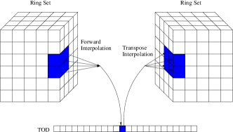
Figure 1: Forward interpolation from ring set to TOD element and transpose interpolation from TOD element to ring set.

PReBeaM also includes the option to zero-pad during the FFT and inverse FFT steps. This means that the working array (either $T_{mm^{\prime}m^{\prime\prime}}$ or $T_{\Phi_{2},\Theta,m^{\prime\prime}}$) is enlarged and padded with zeroes out to $\ell_{max,pad}>\ell_{max}$. This has the effect of decreasing the sampling interval. We found that the combined effects of small-order polynomial interpolation (order 1 or 3) and zero-padding of $2\times\ell_{max}$ or $4\times\ell_{max}$ dramatically reduced the residuals in our maps.

2.4 Parallelization Description

PReBeaM employs a hierarchical parallelization scheme using both shared-memory (OpenMP) and distributed-memory (MPI) types of parallelization. The map-making was performed on the NERSC computer Bassi. Bassi processors are distributed among compute nodes, with 8 processors per node. OpenMP tasks occur within a node and MPI tasks occur between nodes.

We show a diagram of our hybrid parallelization scheme in Figure 2. The full TOD and pointings are divided equally between the nodes for input and storage of pointings. Within an iteration loop, four head nodes are designated to perform the convolutions, while the remaining active nodes are dedicated to the interpolation routines. Each of these four nodes performs the convolution of the sky with one of the four detectors. The resulting arrays are then distributed to all nodes for interpolation over the segment of data stored there and then gathered back onto the designated nodes for transpose convolution. Finally, the $a_{\ell m}$ are summed, using MPI task mpi_reduce, into a single $a_{\ell m}$ on a single node; this is the new estimate for the sky vector.

Figure 2: Depiction of hybrid parallelization scheme used in PReBeaM. Rectangles represent work done on a node, ellipses represent data products, and arrows represent transfer of data. The work done within a node (convolution, interpolation and their transpose operations) is parallelized using OpenMP. This shows a slice of two head nodes though the algorithm may operate on many more nodes.

This particular scheme was devised so that the four distinct convolutions that must occur (one sky with four different beams) can take place simultaneously, while the pointings are distributed among as many nodes as possible for maximum speed in interpolation. Both convolution and interpolation and their transpose operations make use of all processors on a node by using OpenMP directives.

3 Simulations and Beams

The simulated Planck data on which PReBeaM was run was generated by the Planck CTP working group for the study of the performance and accuracy of five map-making codes summarized in the Trieste paper (Ashdown et al., 2008). Planck will spin at a rate of approximately one rpm, with an angle between the spin axis and the optical axis of $\sim 85^{\circ}$. We used the cycloidal scan strategy in which the spin axis follows a circular path with a period of six months, and the angle between the spin axis and the anti-Sun direction is $7.5^{\circ}$. TODs were generated for 366 days for the four 30 GHz Low Frenquency Instrument (LFI) detectors. At a sampling frequency of 32.5 Hz, this corresponds to 1.028x$10^{9}$ samples per detector, for a total of over 65 Gb of data and pointings. The simulated data also included the effects of variable spin velocity and nutation (the option to include the effects of a finite sampling period was not included).

The data was simulated with elliptical having with a geometric mean FWHM of $32.^{\prime}1865$ and ellipticity (maximum FWHM divided by minimum FWHM) of 1.3562 and 1.3929 for each pair of horns. The widths and orientations of the beams were different; this was referred to as beam mismatch in the Trieste paper. In spherical harmonic space, the simulation beams were described up to a beam $m_{max}$ of 14. The same beams were used in PReBeaM to solve for the map, although we allowed the beam asymmetry parameter $m_{max}$ to vary.

4 Results and Discussion

For this paper, we make temperature and polarization maps from simulated one-year observations of the four 30 GHz detectors of the Planck LFI. We examine two cases: CMB signal only and CMB plus uncorrelated (white) noise. Foreground signals and correlated noise properties will be examined in a future paper. The 30 GHz data was an optimal choice for this analysis because the low sampling rate and resolution minimize the data volume, while the large beam ellipticity allows us to demonstrate the full potential of our beam deconvolution technique.

PReBeaM operates entirely in harmonic space, solving for and producing as output $a_{\ell m}$. For visualization purposes, maps were made from $a_{\ell m}$’s out to $\ell_{max}$ 512 and at the Healpix (Gorski et al., 2005) resolution of nside 512 ($\sim 7^{\prime\prime}$ pixel size). Most of the results presented in this paper were attained with an FFT zero-padding of factor four, an interpolation order of 3, and an asymmetry parameter of $m_{max}=$4 (we note where the parameters differ from this). To compare with the input signal, a reference map representing the true sky was created by smoothing the input $a_{\ell m}$ by a Gaussian beam of FWHM = $32.^{\prime}1865$. Similarly, our regularizer $G$ (in equation (2)) was set to have a FWHM of $32.^{\prime}1865$ to match this smoothing. As noted in §3, the same data we use here has been processed by five map-making codes in Ashdown et al. (2008). We have chosen to compare our results with the analogous results from Springtide, one of the codes in this study. Springtide was chosen, out of the five codes, because it is the map-making code installed in and used by the Planck Data Processing Centers for the HFI and LFI instrument. It is sufficient to compare with Springtide only as no significant differences in accuracy were found between codes (with similar baselines and in the absence of noise) (Ashdown et al., 2008). In the absence of noise, Springtide is algorithmically akin to a straight-forward binning of the TOD into a sky pixel map. Because we are using Springtide to represent all non-beam-deconvolution methods we will refer to the Springtide maps as the binned maps.

We begin by examining the spectra in the binned map, PReBeaM map and the smoothed input map shown in Figure 3. The effect of the beam mismatch is clearly seen where the peaks and valleys of the binned map spectra have been shifted towards higher multipoles. The detectors measure different Stokes I which translates to artifacts in the polarization map. Deconvolution suppresses leakage from temperature to polarization as evidenced by the PReBeaM spectra which overlays the input spectra. This shift is expected to remain apparent in the TE spectra of non-beam-deconvolved maps even in the presence of noise because of larger temperature signal and the temperature-to-polarization cross-coupling.

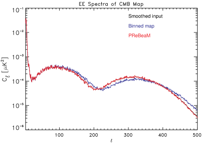
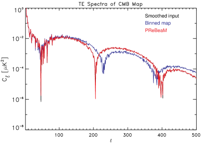
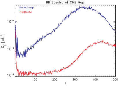
Figure 3: EE, TE, and BB spectra of smoothed input map (black curve), binned map (blue curve) and PReBeaM (red curve). The EE and TE spectra show the effect of temperature-to-polarization cross-coupling seen in the binned map spectra as shifts in the peaks and valleys and absent from the PReBeaM spectra. The input BB spectra is absent from the BB plot since the input B-modes were zero. TT spectra are omitted since differences in the three spectra are not apparent in this representation.

The fractional difference in the angular power spectrum (defined as $(C_{\ell_{out}}-C_{\ell_{in}})/C_{\ell_{in}}$) of the input and output maps is shown in Figure 4. We show the fractional difference spectra for the TT, EE, and cross-correlation TE signals, omitting the BB spectra since $C^{BB}_{\ell}$ is zero in the simulation of the CMB map . The results for PReBeaM are shown at three intervals: the 25th, 50th and 75th iterations. This shows the behavior of the power spectra as PReBeaM converges on the solution. The beam mismatch effect is also seen in Figure 4, where the fractional difference in the PReBeaM spectra lie closer to zero than the binned map spectra over the full range of multipole moments for EE and TE.

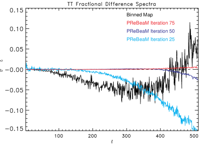
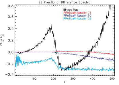
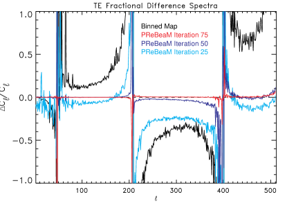
Figure 4: Fractional difference in power spectrum for PReBeaM (red, blue, and cyan curves) and the binned map (black curve) for TT, EE, and TE. Spectra for PReBeaM are shown as a function of number of iterations to demonstrate convergence.

As described earlier, PReBeaM allows for variation in the asymmetry parameter $m_{max}$. We examined the performance of PReBeaM as a function of $m_{max}$, setting it to 2, 4 and 6. A remarkable improvement in the power spectra was found by increasing $m_{max}$ from 2 to 4, while an increase from 4 to 6 only resulted in marginal improvements. This effect is best seen in the BB power spectra as shown in Figure 5. Thus, while the input TOD was simulated with a beam having an $m_{max}$ cut-off of 14, PReBeaM operates optimally at an $m_{max}$ of just 4, thereby allowing us to capitalize on the computational property that PReBeaM scales as $m_{max}$.

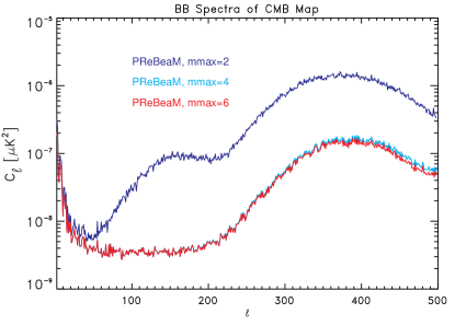
Figure 5: BB power spectra as a function of asymmetry parameter $m_{max}$ for $m_{max}=$ 2 (blue curve) , 4 (cyan curve), and 6 (red curve). The input BB spectra was zero so the smallest output BB spectra is most desirable. In this run, the PReBeaM input parameters interpolation order and zero-padding were set to 1 and 2, respectively.

We define a quantity called $n_{\sigma}$

$$n_{\sigma_{\ell}}=\sum_{\ell^{\prime}=2}^{\ell}\frac{|\Delta C_{\ell^{\prime}}|}{\sigma_{Planck_{\ell^{\prime}}}}$$ (10)

which we use to quantify the maximum, or worst-case bias beam systematics could induce in a cosmological parameter that happened to be degenerate with that parameter. The quantity $\sigma_{Planck}$ is the expected one-sigma errors for the LFI 30 GHz channel, computed as the diagonal elements of the covariance matrix for the simulated input spectra, assuming a sky fraction of 0.65. The $n_{sigma}$ values are plotted in Figure 6 and show that PReBeaM reduces the worst case bias due to untreated beam systematics from tens of sigma to much less than one sigma over the entire $\ell$ range.

Figure 6: Worst case bias in estimation of cosmological parameters due to errors in the power spectra of PReBeaM (dashed curve) and due to the errors in the power spectra of the binned map (solid curve).

We examine the resulting temperature and polarization (Q and U) maps. The output map for both PReBeaM and the binned map was subtracted from the smoothed input map at the same resolution to make the residual maps shown in Figure 7. PReBeaM residuals were plotted on the same color scale as the binned map, showing that PReBeaM attained smaller residuals for both temperature and polarization.

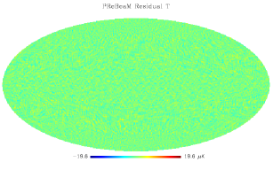
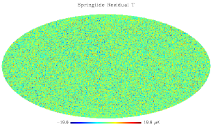
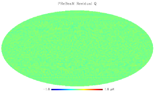
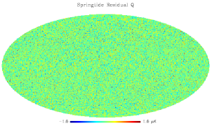
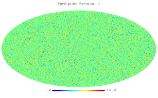
Figure 7: The residuals between the input reference sky and PReBeaM output (left column) and the residual between the input reference sky and the binned map (right column) for Temperature (T), and the Stokes Q, and U parameters.

As a final test, we run PReBeaM on TOD containing CMB signal and white noise and compare with the smoothed input CMB spectrum and the analogous results from Springtide (in this case we refer to Springtide directly since this is not simply a binned map). The level of the uncorrelated noise is specifed in the detector database and has a nominal standard deviation per sample time of $\sigma=1350\mu K$ (Ashdown et al., 2008). PReBeaM achieves a noticeably superior fit to the input spectrum compared with Springtide from $\ell\sim 150$ to $\sim 250$. Assessing the relative performance of PReBeaM and Springtide in more detail would require performing Monte Carlo averages. We focus on the TE spectrum since the improvement is visible even for a single simulation. For the other spectra PReBeaM performs as least as well as Springtide but the detailed difference are more difficult to assess without a Monte Carlo study.

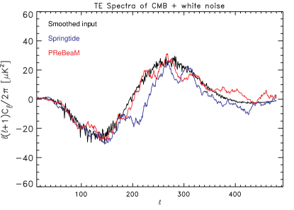
Figure 8: TE spectrum of CMB and white noise for Springtide (blue curve) and PReBeaM (red curve). The smoothed input map is shown in black. Following the example in Ashdown et al. (2008), we reduce $\ell$ to $\ell$ variation by filtering the spectra by a sliding average ($\Delta\ell=20$). In this run, the PReBeaM input parameters interpolation order and zero-padding were set to 1 and 4, respectively. While PReBeaM performs at least as well as Springtide in the TT, EE, and BB spectra, we omit these spectra since the detailed differences are difficult to assess without an in-depth Monte Carlo study.

4.1 Computational Considerations

The computational costs and advantages of our method should be noted. To perform a convolution up to $\ell_{max}$ requires $\mathcal{O}(\ell^{3}_{max}m_{max})$ for the general case. Since $m_{max}$ is bounded by $\ell_{max}$, the cost never scales worse than $\mathcal{O}(\ell^{4}_{max})$ and is only $\mathcal{O}(\ell^{3}_{max})$ for the symmetric beam case. By comparison, a brute force computation in pixel space would require $\mathcal{O}(\ell^{5}_{max})$. In this study, data was simulated with beams having an asymmetry parameter of $m_{max}=14$, but maps were made using a cut-off value of $m_{max}=4$ in PReBeaM. We have demonstrated that computational cost can be conserved while still achieving the benefits of beam deconvolution

It was found that an increase in the zero-padding factor from two to four produced superior results over an increase in the interpolation order from one to three. An optimal run of PReBeaM will therefore include the largest zero-padding possible given machine memory constraints in conjunction with a polynomial interpolation of order one or three. This is advantageous since the time spent in an FFT is nearly negligible and affected only minimally with an increase in zero-padding. In contrast, time for interpolation scales as interpolation-order-squared and as this is a TOD-handling step, it dominates over any cost incurred by convolutions. In the case of the results shown here, interpolation steps consume more than 90% of the wall-clock time per iteration.

The results produced here were generated using 12 nodes on NERSC computer Bassi (making use of all 8 processors per node) and was complete in about 29 wall-clock hours, for a total of 2797-CPU hours. The maximum task memory was 20 GB on a single node.

5 Conclusion

We have found that PReBeaM has outperformed the standard binned noiseless map using two measures: spectra and residual maps. We examined the fractional differences in the spectra and found markedly smaller differences in the PReBeaM spectra versus the binned map spectra across a range of multipole moments. We find that map-making codes which do not deconvolve beam asymmetries lead to significant systematics in the polarization power spectra measurements. The temperature-to-polarization cross-coupling due to beam asymmetries is manifested as shifts in the peaks and valleys of the spectra. These shifts are absent from the PReBeaM spectra. We translated the errors found in the power spectra to an estimate of the statistical significance of the errors in a parameter estimation resulting from these spectra, which we call $n_{\sigma}$. This analysis showed that the worst case parameter bias due to beam-induced power spectrum systematics could be tens of sigma while PReBeaM reduces the risk of parameter bias due to beam systematics to much less than 1 sigma We also found the I, Q, and U component residual maps to be smaller for PReBeaM than for the binned map, implying smaller map-making errors.

We have presented here the first results from PReBeaM for a straightforward test cases of CMB only and CMB plus white noise, and including only the effects of beams in the main focal plane. However, there is great potential for using PReBeaM to remove or assess systematics due to the combination of foregrounds and beam side lobes. Systematics introduced by side lobes will appear on the largest scales, potentially impeding the detection of primordial B-modes on the scales where they are most likely to be measured. We have already shown for temperature measurements (Armitage & Wandelt, 2004) that our deconvolution technique can be used to remove effects due to side lobes. Future work will examine the noise properties of PReBeaM maps and will include foregrounds from extragalactic sources and diffuse Galactic emission.

References

- Armitage & Wandelt (2004) Armitage, C., & Wandelt, B. 2004, Phys. Rev. D 70, 123007
- Ashdown et al. (2008) Ashdown, M. A. J. et al. 2008, submitted to AA, astro-ph 0702483
- Challinor et al. (2000) Challinor, A. et al 2000, Phys. Rev. D 62, 123002
- Gorski et al. (2005) Górski, K. et al 2005, “The HEALPix Primer” (Version 2.00), available at http://healpix.jpl.nasa.gov
- Harrison et al. (2008) Harrison, D. L., van Leeuwen, F., and Ashdown, M. A. J. 2008, in preparation
- Mitra et al. (2007) Mitra, S., et al. 2007, astro-ph 0702100
- The Planck Collaboration (2005) The Planck Collaboration 2005, ESA-SCI(2005)-1., astro-ph 0604069v1
- Reinecke et al. (2006) Reinecke, M. et al. 2006, A&A, 445, 373
- Souradeep et al. (2006) Souradeep, T. et al. 2006, New A Rev., 50, 1030
- Wandelt & Gorski (2001) Wandelt, B. & Górski, K. 2001, Phys. Rev. D 63, 123002