Effects of intersegmental transfers on target location by proteins

Abstract

We study a model for a protein searching for a target, using facilitated diffusion, on a DNA molecule confined in a finite volume. The model includes three distinct pathways for facilitated diffusion: (a) sliding - in which the protein diffuses along the contour of the DNA (b) jumping - where the protein travels between two sites along the DNA by three-dimensional diffusion, and finally (c) intersegmental transfer - which allows the protein to move from one site to another by transiently binding both at the same time. The typical search time is calculated using scaling arguments which are verified numerically. Our results suggest that the inclusion of intersegmental transfer (i) decreases the search time considerably (ii) makes the search time much more robust to variations in the parameters of the model and (iii) that the optimal search time occurs in a regime very different than that found for models which ignore intersegmental transfers. The behavior we find is rich and shows surprising dependencies, for example, on the DNA length.

I Introduction

Many biological processes depend on the ability of proteins to locate specific DNA sequences on time scales ranging from seconds to minutes. Examples include gene expression and repression, DNA replication and others ABLRRW94 . Naively, one might expect the protein to search for its target using only three-dimensional diffusion. Neglecting interactions of the protein with the environment and the DNA (apart from the target site) one then finds, using results first obtained by Smoluchowski S17 , that the average search time, $t^{search}$, is given by:

$$t^{search}\sim\frac{\Lambda^{3}}{D_{3}r}\;.$$ (1)

Here $D_{3}$ is the three-dimensional diffusion constant of the protein, $r$ is the target size and $\Lambda^{3}$ is the volume that needs to be searched. Assuming a target size of the order of a base-pair $r\approx 0.34nm$, a typical nucleus (or bacteria) size of $\Lambda\sim 10^{3}nm$ and using the measured three-dimensional diffusion coefficient for a GFP protein in vivo, $D_{3}\sim 10^{7}{nm}^{2}/s$ ESWSL99 , one finds $t^{search}$ of the order of hundreds of seconds. If $N$ proteins are searching for the same target the search time is given by $t_{N}^{search}\simeq t^{search}/N$. This suggests that about $10$ proteins could find a target in reasonable times for cells to function properly.

In real systems, due to the interactions of proteins with non-specific DNA sequences and the environment LR72 , the picture is more complex. Indeed, in vitro experiments have suggested that mechanisms other than three-dimensional diffusion are used by many proteins to locate their targets RSB70 ; RBC70 . These strategies have been studied and debated extensively both in the context of in vivo BWH81 ; SM2004 ; HGS2006 ; HS2007 and in vitro systems BB76 ; BWH81 ; HM2004 ; BZ2004 ; Z2005 ; LAM2005 ; HGS2006 and are believed, in general, to allow for search times which are faster than that given by Eq. (1).

Historically, the first strategy that was proposed combines one-dimensional diffusion (sliding) over the DNA with intervals of three-dimensional diffusion (typically called jumping in this context) AD68 ; BWH81 (see Fig. 1). Each individual search mechanism, when applied alone, has shortcoming and advantages over the other. When using only three-dimensional diffusion, the number of new three dimensional positions probed grows linearly in time but the protein spends much time probing sites where there is no DNA present. In contrast, during one-dimensional diffusion the protein is constantly bound to the DNA but suffers from a slow increase in the number of new positions probed as a function of time ($\sim t^{1/2}$, where $t$ denotes time) H95Volume1 . As shown, for example, in Refs. AD68 ; BWH81 by intertwining one and three dimensional search strategies and tuning the properties of both one can in fact decrease the search time significantly.

The combined strategy, while better than the pure search strategies, comes at a cost of being sensitive to changes in the properties of either the three-dimensional or one-dimensional diffusive processes. For example, as we argue below, the typical search time changes exponentially in the square root of the ionic strength. Moreover, given the many constraints on the protein to function it is very restrictive to demand optimization for the search process. Indeed, equilibrium measurements K-HRBOCNVH77 and recent single molecule experiment WAC2006 ; ELX2007 on the Lac repressor protein suggest that the search process may not be in general optimized for this search strategy.

A third mechanism which was suggested to speed the search time is intersegmental transfer (IT) HRGW75 ; BC75 . During an IT the protein moves from one site to another by transiently binding both at the same time. In principle the new site can be either close along the one-dimensional DNA sequence (or chemical distance) or distant (see Fig. 3). This mechanism is likely to be relevant for the proteins that have more than one binding domain like the Lac repressor FM92 ; RC92 , GRdbd LN97 and SfiI enzyme EWWH99 . However, it could also occur in proteins with a single binding site in locations where the DNA crosses itself . To date we are aware of direct evidence for IT only for RNA polymerase BGZY99 . However, measurement of the dissociation rate from a labeled (operator) DNA site of the rat glucocorticoid receptor LN97 , CAP and Lac repressor FC84 revealed significant dependence on the DNA concentration in the solvent, a possible explanation for which is IT.

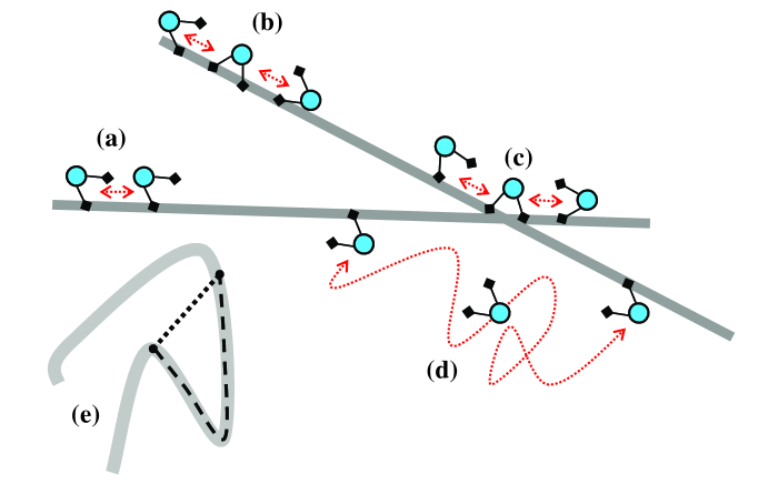
Figure 1: Schematic plots illustrating the different mechanisms that can participate in the facilitated diffusion process. Here dashed arrows represent different protein moves, the solid curve represents the DNA and a small circle with two legs indicates a protein with two binding domains. The figure shows (a) sliding, (b) a correlated intersegmental transfer, (c) an uncorrelated intersegmental transfer, (d) jumping. The distinction between (b) and (c) is defined in Sec. III. (e) The dashed (dotted) line represents a one-dimensional (three-dimensional) distance.

Some theoretical work has suggested that in vivo, when the DNA concentration is much larger than in vitro experiments, IT may play a determinative role BWH81 ; LAM2005 ; HS2007 . These studies focus on the ITs resulting from the DNA dynamics and consider the protein to be point like.

In this paper we present a rather comprehensive study of the effects of ITs on the search process for a DNA molecule confined in a finite volume, similar to the in vivo scenario. Our work complements previous ones by explicitly accounting for the size of the protein and considering two limiting cases: (i) DNA which is completely static during the search process and (ii) DNA whose motion is quicker than that of the protein’s motion along the DNA. Using scaling arguments backed by numerics we obtain expressions for $t^{search}$, and the optimal search time (obtained by tuning parameters such as the DNA-protein affinity). A central conclusion of this paper is that the search time is much more robust to variations in parameters when ITs are allowed. This is to the extent that in some cases any finite jumping rate can have a negative influence on the search time. In particular, the optimal search time is found to occur for parameter regimes very different than the canonical one (see Sec. II) found in models which ignore ITs. Perhaps most important, as we show, our work suggests that ITs could explain recent findings which indicate a much higher affinity of the TF Lac repressor to the DNA than required by an optimal search strategy which uses only sliding and jumping WAC2006 ; ELX2007 ; K-HRBOCNVH77 .

The scaling dependence of the search time on different parameters is rich and very different from regular facilitated diffusion (involving only sliding and jumping). Consider, for example, the dependence of the search process on the length of the DNA, $L$ for a DNA confined in a volume $\Lambda^{3}$. Using only sliding and jumping the regime typically thought to be relevant to experiment has a linear dependence of the search time on the DNA length $L$. A Smoluchowski-like search time is independent of $L$. In contrast, when ITs are allowed we find different behavior. We estimate that the regime most relevant to in vivo experiments (in prokaryotic organisms) occurs when the dependence on the length of the DNA is weak. For example, when a searches are performed using only ITs the search time can be independent of $L$ or scales as $\sqrt{L}$ depending on the DNA’s dynamics. The scaling behaviors relics on the confinement of the DNA in a finite volume (shown in detail in Fig. 9) and could be used as experimental probes for the existence of ITs.

The paper is organized as follows: Sec. II briefly reviews the main arguments used to analyze searches that combines only sliding and jumping. In Sec. III the average search time is calculated for the case of a strategy based only on ITs for both quenched and annealed DNA. In Sec. IV a search process that includes ITs and sliding is considered. Sec. V considers the possibility that the protein can unbind from the DNA (jump) and perform ITs. Sec. VI studies a model with all three mechanisms. Finally, in Sec. VII we discuss possible scenarios for the Lac repressor and summarize in Sec. VIII.

II Sliding and jumping

To set the stage for a discussion of the effects of IT we consider a search process which uses only sliding and jumping. The discussion follows Refs. SM2004 and HM2004 closely. We imagine a single protein searching for a single target located on the DNA. The search is composed of a series of intervals of one-dimensional diffusion along the DNA (sliding) and three-dimensional diffusion in the solution (jumping). The typical time of each is denoted by $\tau_{1}$ and $\tau_{3}$ respectively. Following a jump, the protein is assumed to associate on a new randomly chosen location along the DNA. While this approach is somewhat simplistic for jumps occurring in two-dimensions and below, for three dimensions, which case we consider, it is well suited CBTVK2007 .

Under these assumptions, during each sliding event the protein covers a typical length $l$, where $l\sim\sqrt{D_{1}\tau_{1}}$ (often called the antenna size) H95Volume1 . Since correlations between the locations of the protein before and after the jump are neglected, the search process, completed when roughly all the DNA is scanned, is separated into

$$N_{r}\sim\frac{L}{l_{s}}$$ (2)

rounds of sliding and jumping. Here $l_{s}$ is the typical length scanned by the protein during a round. If during the slide the protein does not skip sites on the DNA $l_{s}\sim l$ (the distinction between $l_{s}$ and $l$ will become apparent when ITs are introduced). The total time needed to find a specific site is then:

$$t^{search}=N_{r}\tau_{r}\;,$$ (3)

with $\tau_{r}=\tau_{1}+\tau_{3}$. Using Eqs. (2) and (3) one obtains

$$t^{search}\sim\frac{L}{l_{s}}(\tau_{1}+\tau_{3})\sim\frac{L}{\sqrt{2D_{1}}}\left(\sqrt{\tau_{1}}+\frac{\tau_{3}}{\sqrt{\tau_{1}}}\right)\;.$$ (4)

Furthermore, it is easy to argue (see Appendix A) that

$$\tau_{3}\sim\frac{\Lambda^{3}}{D_{3}L}\;.$$ (5)

In Fig. 2 a comparison between the presented scaling arguments and a numerical simulation of a search that explicitly includes sliding on a DNA with a frozen configuration in a finite volume and three dimensional diffusion is shown (see Appendix B for details of the numerics). The excellent agreement justifies many of the simplifications made, in particular, the neglect correlation between the initial and final location of the jump. Throughout the  paper we assume this always holds (see Appendix B).

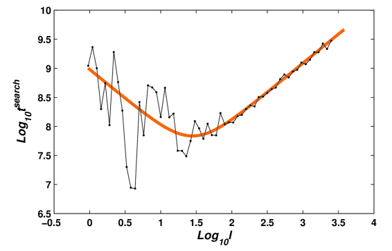
Figure 2: The search time $t^{search}$ is shown as a function of the antenna length, $l$. The thin line represents the results from numerical simulations while the bold one is given by Eq. (4). Numerics were performed on a DNA embedded in a finite volume with a frozen configuration. The length of the DNA was taken to be $1224000$ lattice constants and $D_{3}=D_{1}=1$ (see details in Appendix B). Similar results were obtained for different values of $D_{1}$ and $D_{3}$.

The analysis leads to a richer range of possible behaviors than found in Eq. (1), where the search time depends only on the volume in which the DNA is embedded HGS2006 . Here, in contrast, three regimes are found: (i) For $\tau_{1}\ll\tau_{3}$ there is no dependence on $L$ and the search time is given to a good approximation by Eq. (1). (ii) For $\frac{L^{2}}{D_{1}}\gg\tau_{1}\gg\tau_{3}$ the dependence on the DNA length is linear. This is the regime typically considered relevant for experiments. (iii) For $\frac{L^{2}}{D_{1}}\ll\tau_{1}$ one finds $t^{search}\propto L^{2}$.

It is natural to ask which $\tau_{1}$ optimizes $t^{search}$. Using Eq. (4) it is easy to verify that

$$\left(\tau_{1}^{opt}\right)_{0}=\tau_{3}\;,$$ (6)

where $0$ denotes a value obtained with no ITs. Alternatively, one can consider an optimal antenna size $(l_{opt})_{0}=\sqrt{2D_{1}\tau_{3}}$. When this condition is met, the total search time scales as

$$t_{opt}^{search}=\sqrt{\frac{\tau_{3}}{D_{1}}}L\sim\sqrt{\frac{\Lambda^{3}L}{D_{1}D_{3}}}\;.$$ (7)

Note that the $\sqrt{L}$ dependence is obtained by optimizing, say $\tau_{1}$, as $L$ is varied.

This model, at the optimal $\tau_{1}$ and assuming known values for $D_{1}$, $L$ and $\tau_{3}$, predicts reasonable search times in vivo and is commonly assumed to give a possible explanation for the two order of magnitude difference between the experiments in vitro and Eq. (1).

Within the model the optimal search process requires fine tuning of the antenna size, $l$, as a function of the parameters $D_{1}$ and $\tau_{3}$. These parameters depend on various cell and environmental conditions such as the size of the cell, the DNA length, the ionic strength etc. The dependence can be quite significant: for example, the parameter $\frac{\tau_{3}}{\tau_{1}}$ has an exponential dependence on the square root of the ionic strength LR75 . Deviations of this parameter from the optimum value might be crucial to the search time since $\frac{t^{search}}{t_{opt}^{search}}=\frac{1}{2}\left(\sqrt{\frac{\tau_{3}}{\tau_{1}}}+\sqrt{\frac{\tau_{1}}{\tau_{3}}}\right)$. Indeed, a strong dependence of the search time on the ionic strength was found in in vitro experiments RBC70 . Interestingly, in vivo, when the DNA is densely packed, no effect of the ionic strength on the efficiency of the Lac repressor was revealed RCMKAFR87 . Other experiments also suggest that $\tau_{1}$ is not optimized. In particular, equilibrium measurements K-HRBOCNVH77 , as well as recent single molecule experiment WAC2006 ; ELX2007 , find a value of $\tau_{1}$ for dimeric Lac repressor that is much larger than the predicted optimum $\tau_{3}$ in vivo.

The lack of sensitivity to the ionic strength in vivo and the rapid search times found for the Lac repressor, even with very large values of $\tau_{1}$, suggest that other processes, apart from jumping and sliding, are involved in the search process. These seem to be more important in vivo than in vitro. In the next section we show that a search process which uses ITs modifies the behavior found for searches which use only sliding and jumping in a significant manner. In particular the problems encountered above (e.g., high sensitivity to the antenna length, very long and non-optimal measured antennas etc.), are largely eliminated when ITs are included.

III Pure intersegmental transfer

Before turning to the full problem of a search which uses sliding, jumping and ITs we will consider a series of simplified models. Within the first model, considered in this section, the protein can only perform ITs. We will see that already at this level many of the problems of the search discussed above, which uses only sliding and jumping, are resolved to a large extent.

To model ITs we consider a protein with two binding sites. The protein can either have one site bound to the DNA or perform an IT to a new location by having both binding sites bound to the DNA (see Fig. 1). The DNA is scanned for the target by the binding sites, each checking a length $b$ when bound (note that since the protein has to align with the DNA sequence, $b$ is of the order of a length of a single base-pair). A possible motivation for this picture is, for example, the tetrameric structure of the Lac repressor. However, as will be evident many results also apply to proteins with different shapes.

Motivated by DNA in cells, we consider a DNA molecule which is densely packed in a small volume. In typical systems the DNA has a total length of $L\sim 10^{6}nm$, a persistence length $L_{0}\sim 50nm$, a cross section radius $\rho\sim 1nm$ and is contained in a volume of $\Lambda^{3}\sim 10^{9}nm^{3}$. The typical distance between segments of DNA of length $L_{0}$ is therefore much smaller than $L_{0}$: $\frac{\Lambda^{3}}{L/L_{0}}\ll L_{0}^{3}$. Under these conditions, using $\Lambda\gg L_{0}$, it is easy to check that the radius of gyration of free DNA, which is of the order of $L_{0}\sqrt{\frac{L}{L_{0}}}$ is much larger than the cell size $\Lambda$ - the DNA is densely packed even though its fractional volume, $L\rho^{2}/\Lambda^{3}$, in the container is small (about one percent). By way of comparison, typical protein sizes are in the range $R\mathbf{\sim}1-10nm$, much smaller than the DNA’s persistence length. Although in vivo the packing has a more complicate structure than we consider, we expect similar behavior to occur also there.

As stated above the protein moves by first being bound with only one binding site and then with both. The typical time for this, defined by $\delta=\tau_{b}+\tau_{IT}$, is the sum of the typical time that protein probes a length $b$ (by being bound with one domain) and the time that the protein is bound with both binding domains to the DNA while performing an IT. We assume that the protein moves (for example, using both legs of the Lac repressor) to a random position located at a distance smaller or equal to $R$, the size of the protein, from it (see Fig. 1). Defining a “chemical” coordinate $x$ which runs along the length of the DNA the protein can either perform moves from its location $x$ to the interval $[x-R,x+R]$ (we refer to these as “correlated ITs” (CITs)) or reach distant sites along the chemical coordinate available through the structure of the packed DNA.

Under the above conditions it is easy to verify (see Appendix C) that almost all ITs performed by the protein are either correlated moves or performed to a coordinate along the DNA whose distance from its previous location is bigger than $\frac{\Lambda^{2}}{L_{0}}$ (but smaller than $L$). We call these steps “uncorrelated ITs” (UITs) (see Fig. 1(c)). In other words, one can safely neglect the possibility that the protein will move using ITs to a chemical distance larger than $R$ and smaller than $\frac{\Lambda^{2}}{L_{0}}$.

Our main interest is the typical search time. For this purpose it is useful to define $\lambda$ - the average length that the protein travels before performing an UIT. On chemical distances larger than $R$ but smaller than $\lambda$ the motion is effectively diffusive in one dimension with a diffusion coefficient $D_{1eff}$ $\sim\frac{R^{2}}{\delta}$. On chemical distance scales larger than $\lambda$ and smaller than $L$ the motion is controlled by UITs. Due to the three-dimensional nature of each UIT one expects correlations between different UITs to be negligible. We verify this assumption later using numerical simulations.

From the discussion and using a language similar to that of Sec. II the search process can be described as a sequence of

$$N_{r}\sim\frac{L}{l_{s}}$$ (8)

rounds of correlated ITs where $l_{s}$ is the length scanned by the protein during each round (namely between two subsequent UITs). The typical time of each round is

$$\tau_{r}\sim\frac{\lambda^{2}}{D_{1eff}}\sim\left(\frac{\lambda}{R}\right)^{2}\delta\;.$$ (9)

In general while performing CITs the protein can miss regions of the DNA by skipping over them. Since each segment of size $R$ is visited $\sqrt{\frac{\tau_{r}}{\delta}}\sim\frac{\lambda}{R}$ times H95Volume1 , when $\frac{\lambda}{R}\gg\frac{R}{b}$ the walk is recurrent and no sites are skipped so that $l_{s}\sim\lambda$. In contrast, when $\frac{\lambda}{R}\ll\frac{R}{b}$ the walk is not recurrent and $l_{s}\sim\frac{\lambda}{R/b}\frac{\lambda}{R}\sim\frac{\lambda^{2}}{R^{2}}b$. Therefore the recurrence length,

$$l_{R}\sim\frac{R^{2}}{b}\;,$$ (10)

separates between two regimes

$$l_{s}\sim\left\{\begin{array}[c]{c}\frac{\lambda^{2}}{l_{R}}\hskip 36.135pt\lambda\ll l_{R}\\ \lambda\hskip 43.36243pt\lambda\gg l_{R}\end{array}\right.\;,$$ (11)

the first transient and the second recurrent.

Using Eqs. (3), (8), (9) and (11) the typical search time is obtained

$$t^{search}\sim\frac{L}{l_{s}}\left(\frac{\lambda}{R}\right)^{2}\delta\sim\left\{\begin{array}[c]{c}\frac{L}{b}\delta\;\;\;\;\;\;\;\lambda\ll l_{R}\\ \frac{L\lambda}{R^{2}}\delta\;\;\;\;\;\;\lambda\gg l_{R}\end{array}\right.\;.$$ (12)

To complete the expression one needs to evaluate $\lambda$. Its value depends on various parameters and, in particular, the time scale which characterize the motion of the DNA. As discussed in the introduction we consider two extreme regimes - quenched DNA and annealed DNA. In both cases $\lambda$ can be evaluated from an intermediate quantity, $p$, the probability that the protein can make an UIT from a specific location $x$ on the DNA. Since this quantity is independent of the DNA’s motion we estimate it first before turning to the two regimes.

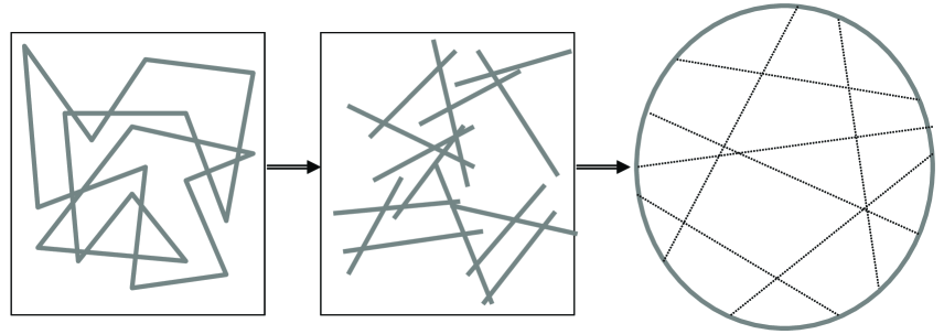
Figure 3: Illustrated schematically is the simplified treatment of the folded DNA. We first represent the DNA as the ideal gas of rods each with of a length of one persistence length. Then we connect the rods randomly to form a small world network (see text for details). Numerically we find the description to work well.

To do so, we consider a packed DNA as an ideal gas of $\frac{L}{L_{0}}$ straight rods of length $L_{0}$ that are distributed randomly in the cell (see Fig. 3). The probability $p_{seg}$, that two given rods cross within a distance of $R$ from each other is given by

$$p_{seg}=A\frac{L_{0}^{3}}{\Lambda^{3}}\frac{R^{2}}{L_{0}^{2}}=A\frac{L_{0}R^{2}}{\Lambda^{3}}\;,$$ (13)

where $A$ is a constant of order unity. Here $\frac{L_{0}^{3}}{\Lambda^{3}}$ is the probability that a given segments is located within a distance $L_{0}$ of a point inside the cell and $\frac{R^{2}}{L_{0}^{2}}$ is proportional to the probability that this segment crosses a sphere of radius $R$ around the point. Under the conditions described above we find that typically $p_{seg}\ll 1$. Finally, to relate $p$ to $p_{seg}$ we note that to make an IT at least one segment should be accessible. This yields

$$p=1-\left(1-p_{seg}\right)^{L/L_{0}}\simeq 1-e^{-A\frac{LR^{2}}{\Lambda^{3}}}\;.$$ (14)

Eq. (14) implies that there are two possible regimes depending on the value of $L$

$$p=\left\{\begin{array}[c]{c}A\frac{LR^{2}}{\Lambda^{3}}\ll 1\hskip 36.135ptL\ll L_{c}\\ 1\hskip 50.58878pt\hskip 28.90755ptL\gg L_{c}\end{array}\right.\;,$$ (15)

where

$$L_{c}\sim\frac{\Lambda^{3}}{R^{2}}\;.$$ (16)

In essence when $L\gg L_{c}$ (which can occur for example by having a large protein) $p\simeq 1$ and about half of the ITs are uncorrelated. However, when $L\ll L_{c}$ we have that $p=A\frac{LR^{2}}{\Lambda^{3}}\ll 1$, and most ITs are correlated. The value of $L_{c}$ for the range of parameters of interest is of the order of $10^{7}nm$ for very large proteins ($R$ of order of tens of $nm$, similar to the Lac repressor). Therefore in vivo we expect a relatively large $L_{c}$, so the regime $L\ll L_{c}$ should be relevant.

To summarize the above analysis we note that it effectively represents motion on the DNA, using ITs, as motion on a one-dimensional discrete network. The size of each site on this network is $b$, the scanned length on the DNA during one binding event. Each step on the network takes on average a time $\delta$. During an IT the protein can move from its position, $x$, to a randomly chosen position in the interval $\left[x-R,x+R\right]$ along the chemical coordinate (correlated transfer) with probability $1-p$ or to an uncorrelated site with probability $p$ (uncorrelated transfer). Such networks are commonly referred to as Small World Networks W99SM (see Fig. 3(c)).

To find the relation between $\lambda$ and $p$ one has to consider the dynamics of the DNA. Below we consider two extreme cases (a) a completely quenched DNA configuration and (b) a strongly fluctuating DNA, which we term annealed. A quenched DNA is static throughout the search process. An annealed DNA changes its conformation on time scale much quicker than the motion of the protein.

III.1 Quenched DNA

In this section we derive the search time for a quenched DNA. In particular we will show that it is has a non-trivial behavior as a function of $L$. In the regime that is expected to be relevant in vivo the search time is independent of the DNA’s length (see Fig. 4).

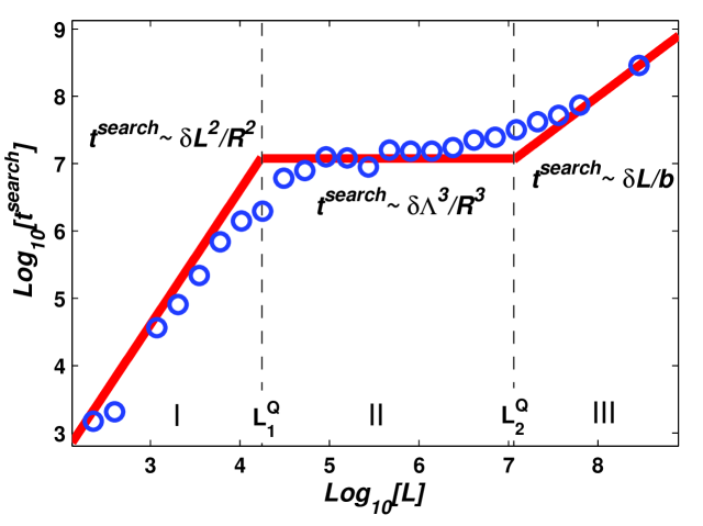
Figure 4: The search time, $t^{search}$, is plotted as a function of $L$, the DNA length for the pure IT case with a quenched DNA configuration. The circles represent numerical data, while the solid line was obtained using Eqs. (21) ,(23) and (24). The three visible regimes correspond to the three on Fig. 5 (see also Fig. 9). In this plot $R$ and $b$ were taken to be $3$ and $1$ lattice constants respectively (the rest of the details are found in Appendix B). The search time is shown in units of $\delta$.

For quenched DNA one expects that if an UIT can occur at point $x$ it can also happen in a region of size $R$ around it. Similar considerations apply to sites where an UIT can not occur. The typical distance traveled by the protein along the DNA’s chemical coordinate between two subsequent UITs, $L>\lambda>R$, is of the order of the typical distance between two distinct locations where an UIT can occur. This implies for $p\gg R/L$ a scaling of $\lambda$ of the form

$$\lambda\sim\frac{R}{p}\;,$$ (17)

where $p$ is defined above (see Eq. (15)) while for $p\ll R/L$ clearly $\lambda=L$ (see Fig. 5).

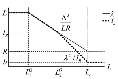
Figure 5: The schematic behaviors of $\lambda$ and $l_{s}$ as a function of $L$ (on a log-log scale) is shown for quenched DNA and $b\ll R$.

From the previous discussion one may infer that there are three distinct behaviors as a function of $L$ shown on Fig. 5. The first regime occurs for DNA so short that an UIT cannot occur during the search. This happens when $p\ll R/L$, or equivalently when  $L\ll L_{1}^{Q}$, where using Eq. (15) one finds

$$L_{1}^{Q}=\sqrt{\frac{\Lambda^{3}}{R}}\;.$$ (18)

In fact, the estimate for $L_{1}^{Q}$ pushes the limit of our treatment since the DNA is no longer densely packed in this regime. Nonetheless, we find good agreement with numerical simulations.

The other regimes occur for $L\gg L_{1}^{Q}$, where one has $p\gg R/L$. In this case the proteins can use UITs during the search. As discussed above there is a length scale $L_{c}$ separating two distinct behaviors of $p$, and therefore we have three different behaviors for $\lambda$ which are given by (see Fig. 5):

$$\lambda\sim\left\{\begin{array}[c]{cc}L&\;\;\;\;L\ll\sqrt{\frac{\Lambda^{3}}{R}}=L_{1}^{Q}\\ \frac{\Lambda^{3}}{LR}&\;\;\;\;L_{1}^{Q}\ll L\ll L_{c}\\ R&\;\;\;\;\;\;L\gg\frac{\Lambda^{3}}{R^{2}}=L_{c}\end{array}\right.\;,$$ (19)

where as before $L_{c}=\Lambda^{3}/R^{2}$. Furthermore, as described above, the scan between two subsequent UIT can either be recurrent ($\lambda\gg l_{R}$) or transient ($\lambda\ll l_{R}$) with a crossover length $L_{2}^{Q}$. This length scale $L_{2}^{Q}$ is determined by the condition $\lambda\left(L=L_{2}^{Q}\right)\sim l_{R}$. In the recurrent regime the walk between two ITs doesn’t skip locations on the DNA. This is in contrast to the transient regime where many sites are skipped. Thus using Eqs. (15) and (17) one finds

$$L_{2}^{Q}=\frac{\Lambda^{3}}{R^{3}}b\;.$$ (20)

For $L\gg L_{2}^{Q}$ the search between two subsequent UITs is short and therefore transient while for $L\ll L_{2}^{Q}$ the search between two subsequent UITs is long and therefore recurrent.

Note that when the search is transient, $t^{search}$ is independent of $\lambda$ (see Eq. (12)). Therefore, the crossover between two distinct scaling behaviors of $t^{search}$ is governed by the smaller of the two length scales $L_{c}$ and $L_{2}^{Q}$. For proteins performing only ITs one expects $b$ to be smaller than $R$. It is easy to see that in such cases $L_{2}^{Q}$ is smaller than $L_{c}$. (Other possibilities are discussed in Sec. IV.)

To summarize there are two length scales $L_{1}^{Q}$ and $L_{2}^{Q}$ which separate three possible regimes (see Fig. 5).

• Regime $\mathbf{I}$: $L\ll L_{1}^{Q}$

In this regime $\lambda\sim L$. There are no UITs and Eqs. (11) and (12) give

$$t^{search}\sim\frac{L^{2}}{2D_{1eff}}\sim\frac{L^{2}}{R^{2}}\delta\;.$$ (21)

This regime is clearly not relevant in vivo (using the typical values, $\Lambda\sim 1\mu m$ and $R\sim 10nm$, we find $L_{1}^{Q}\sim 10\mu m$ which is much shorter than typical DNA lengths).

• Regime $\mathbf{II}$: $L_{1}^{Q}\ll L\ll L_{2}^{Q}$

Now the motion between two subsequent UITs is recurrent, $l_{R}\ll\lambda$, and Eq. (17) gives

$$\lambda\sim\frac{\Lambda^{3}}{LR}\;.$$ (22)

Using Eqs. (11) and (12) we obtain

$$t^{search}\sim\frac{\Lambda^{3}}{R^{3}}\delta\;.$$ (23)

Note that in this regime, as opposed to Sec. II, the search time is independent of the DNA’s length. Eq. (23) is equivalent to Eq. (1) with an effective three-dimensional diffusion coefficient $D_{3}\sim\frac{R^{3}}{r\delta}$. In contrast to the simple three-dimensional diffusive search Eq. (23) does not depends on the target size $r$ but rather on the protein size which may be much larger.

• Regime $\mathbf{III}$: $L\gg L_{2}^{Q}$

Here $\lambda\ll l_{R}$. and Eqs. (11) and (12) give

$$t^{search}\sim\frac{L\delta}{b}\;.$$ (24)

The obtained results, compared to numerics, are summarized in Figs. 4 (see also Fig. 9). One can clearly see the three regimes arising for different lengths of DNA which are separated by $L_{1}^{Q}$ and $L_{2}^{Q}$. The details of the numerical simulation are described in Appendix B. Note that $L_{1}^{Q}$ and $L_{2}^{Q}$ are well predicted by the scaling arguments.

The most relevant regime for in vivo experiments in prokaryotic organisms is likely to be the intermediate regime ($\mathbf{II}$) where the search time is independent of the DNA’s length and scales as $\Lambda^{3}$. Comparing the search time in this regime (23) with the minimal search time in the case when sliding and jumping are used, Eq. (7), one may see that if $\delta<R^{3}\sqrt{\frac{L}{\Lambda^{3}D_{1}D_{3}}}$ the search time in the pure IT scenario is in fact smaller than the one of Sec. II which includes only sliding and jumping case. This is despite the fact that the protein never unbinds from the DNA.

III.2 Annealed DNA

In this section we consider the annealed case. As we show, here the search time also has non-trivial but different than the quenched case behavior as a function of $L$. In the regime that is expected to be relevant in vivo the search time scales as $\sqrt{L}$.

In the annealed case the time scale for a rearrangement of the DNA’s configuration is assumed to be much smaller than the time of the protein’s motion during an IT. As a result of the constant rearrangement of the DNA UITs now occur with probability $p$ for each IT. The average number of ITs with no UITs performed is therefore of the order of $\frac{1}{p}$ and thus the average time that the protein spends between two subsequent UITs is $\frac{\delta}{p}$ ($\delta$ as before is the typical time between two subsequent ITs). On one-dimensional length scales smaller than $\lambda$ the protein diffuses with a diffusion constant $D_{1eff}\sim\frac{R^{2}}{\delta}$. Therefore, the typical one-dimensional distance between two subsequent UITs $\lambda$ is

$$\lambda\sim\sqrt{D_{1eff}\frac{\delta}{p}}\simeq\left\{\begin{array}[c]{cc}\sqrt{\frac{\Lambda^{3}}{L}}&\;\;\;\;L\ll L_{c}\\ R&\;\;\;\;L\gg L_{c}\end{array}\right.\;,$$ (25)

where $L_{c}$ is defined in Eq. (16). As for the quenched case we will see that again three distinct behaviors arise with two crossover lengths.

The first occurs when no UITs occur. The crossover length $L_{1}^{A}$ can be extracted using the condition $\lambda\left(L=L_{1}^{A}\right)\sim L$ which under our assumptions on the protein’s size can only occur when $L\ll L_{c}$. This yields

$$L_{1}^{A}\sim\Lambda\;.$$

It is easy to see that $L_{1}^{A}\ll L_{1}^{Q}$. This means that, as expected, in the annealed case the effects of UITs become important at much smaller DNA concentration than in the quenched case. This happens because fast DNA movements increase the probability to perform an UIT. As for $L_{1}^{Q}$, the estimate for $L_{1}^{A}$ pushes the limit of our treatment since the DNA is no longer densely packed in this regime.

The second crossover length $L_{2}^{A}$ occurs when the motion between UITs becomes transient. It can therefore be estimated using $\lambda\left(L=L_{1}^{A}\right)\sim l_{R}$. Taking the regime $L\ll L_{c}$ in Eq. (25) yields

$$L_{2}^{A}\sim\frac{b^{2}\Lambda^{3}}{R^{4}}\;.$$ (26)

For target sizes much smaller than the protein size ($b\ll R$), it is clear that $L_{2}^{A}\ll L_{c}$ (see Eq. (16)). Hence, using the same arguments as before, only two length scales, $L_{1}^{A}$ and $L_{2}^{A}$, determines three possible regimes (see Fig. 6).

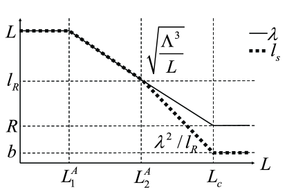
Figure 6: The schematic behavior of $\lambda$ and $l_{s}$ as a function of $L$ (on a log-log scale) is shown for annealed DNA and $b\ll R$.

The three regimes which arise are:

• Regime $\mathbf{I}$: $L\ll L_{1}^{A}$

Here $\lambda\sim L$. There are no UITs and Eqs. (11) and (12) give

$$t^{search}\sim\frac{L^{2}}{2D_{1eff}}\sim\frac{L^{2}}{R^{2}}\delta\;.$$ (27)

• Regime $\mathbf{II}$: $L_{1}^{A}\ll L\ll L_{2}^{A}$

Here searches between two subsequent UIT are recurrent so that $l_{R}\ll\lambda$. Eq. (25) gives

$$\lambda\sim\sqrt{\frac{\Lambda^{3}}{L}}\;.$$ (28)

Using Eqs. (11) and (12) we obtain

$$t^{search}\sim\frac{\sqrt{L\Lambda^{3}}}{R^{2}}\delta\;.$$ (29)

Here, in contrast to the quenched case the intermediate result scales with the length of the DNA as $L^{1/2}$. Note that the search time is always shorter than that on a quenched DNA. This happens because the DNA’s movement destroys the correlation in the motion of the protein and, therefore, increases the efficiency of the search. A similar dependence on $L$ ($t^{search}\propto\sqrt{L}$) was obtained for a different model HS2007 . There, however, the origin of the dependence is different, and is linked to modeling the DNA’s motion as diffusion of an ideal gas of rods.

• Regime $\mathbf{III}$: $L\gg L_{2}^{A}$

Here $\lambda\ll l_{R}$. Therefore, Eqs. (11) and (12) give

$$t^{search}\sim\frac{L\delta}{b}\;.$$ (30)

The obtained results are summarized later in Fig. 9.

The most relevant regime for in vivo experiments in prokaryotic organisms is likely to be the intermediate one ($\mathbf{II}$) where the search time scales as $L^{1/2}$ or alternatively as $\Lambda^{3/2}$. Comparing the search time in this regime (29) with the minimal search time in the case when sliding and jumping are used (7) one may see that if $\delta<\frac{R^{2}}{\sqrt{D_{1}D_{3}}}$ the search time in the pure IT case is smaller than the one in the sliding and jumping case. This is despite the fact that the protein never unbinds from the DNA.

Numerical simulation of the annealed case require dynamical moves for the whole DNA molecule. This is a formidable task for DNAs with reasonable length which is beyond the scope of this paper.

IV Intersegmental transfer and sliding

Next we consider a protein that can perform both ITs and sliding. Namely, in addition to ITs the protein can perform one-dimensional diffusion with only one binding domain bound (see Fig. 1(a)). In the language of Sec. III, $b$ is now the typical sliding length between two subsequent ITs. Now each step (distinct from a round defined above), defined as the interval between the ends of two subsequent ITs, takes a typical time $\delta=\frac{b^{2}}{2D_{1}}+\tau_{IT}$, where $D_{1}$ is the one dimensional diffusion coefficient of the protein with only one binding domain bound and $\tau_{IT}$ is the typical time that the protein is bound to two DNA segments.

If $b\ll R$ it is straightforward to see that the results of the Sec. III hold with a redefined $\delta$. However, in general the sliding length $b$ might be much larger than the proteins size $R$. This is the regime that we focus on in this section.

Clearly, now the search between two subsequent UIT is always recurrent so that $l_{s}\sim\lambda$. Here as before $\lambda$ is the typical distance traveled by the protein between two subsequent UITs. However, now $D_{1eff}$ $\sim\frac{b^{2}}{\delta}$, where as above $\delta=\frac{b^{2}}{2D_{1}}+\tau_{IT}$. The search time as a function of $\lambda$, similar to Eq. (12), becomes

$$t^{search}\sim\frac{L}{\lambda}\frac{\lambda^{2}}{D_{1eff}}\sim\frac{L\lambda}{b^{2}}\delta\;.$$ (31)

The value of $\lambda$, as in the previous section, depends on the dynamics of the DNA molecule. Again we consider two extreme cases (a) quenched DNA and (b) annealed DNA.

IV.1 Quenched DNA

To obtain $\lambda$ we first introduce a new quantity, $\lambda_{0}$, defined as the typical chemical distance between two locations in which the protein can perform an UIT. Note that we are interesting in the regime $b\gg R$. Therefore the values of $\lambda$ and $\lambda_{0}$ may be distinct since an UIT is not necessarily performed at every possible location on the DNA. Clearly, however, the functional behavior of $\lambda_{0}$ is identical to that of $\lambda$ in the previous section. This yields (see Eq. 19)

$$\lambda_{0}\sim\left\{\begin{array}[c]{cc}L&\;\;\;\;L\ll\sqrt{\frac{\Lambda^{3}}{R}}=L_{1}^{Q}\\ \frac{\Lambda^{3}}{LR}&\;\;\;\;L_{1}^{Q}\ll L\ll L_{c}\\ R&\;\;\;\;\;\;\;\;L\gg\frac{\Lambda^{3}}{R^{2}}=L_{c}\end{array}\right.\;,$$ (32)

where we have used the definitions of $L_{1}^{Q}$ and $L_{c}$ of the previous section.

Similar to the derivation of Eq. (10), when $\lambda_{0}/b\gg b/R$, the effective random walk of the protein along a length $\lambda_{0}$ is recurrent. Here recurrent motion implies that sites where an UIT can occur are visited many times before a neighboring site where an UIT can occur is met (note that this is distinct from the recurrent behavior of Sec. III). In the recurrent regime a location of a possible UITs is visited many times and therefore not missed. In this case $\lambda\sim\lambda_{0}$. In the opposite transient regime (again distinct in meaning from that used in Sec. III), $\frac{\lambda_{0}}{b}\ll\frac{b}{R}$ and the protein performs an UIT only after it travels a distance $\lambda\gg\lambda_{0}$. In the latter regime each IT has a probability $\frac{R}{\lambda_{0}}$ to be an UIT. Therefore between two subsequent UITs the protein performs $\frac{\lambda_{0}}{R}$ ITs. Using the diffusive nature of the motion we find $\lambda\sim b\sqrt{\frac{\lambda_{0}}{R}}$. The value of $\lambda$ as function of $\lambda_{0}$ is shown schematically in Fig. 7.

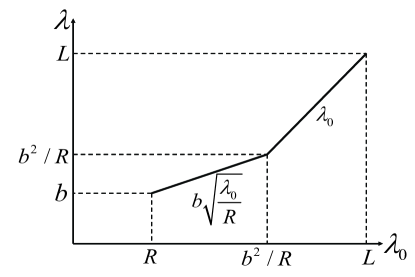
Figure 7: The schematic behavior of $\lambda$ and $l_{s}$ as a function of $L$ (on a log-log scale) is shown for quenched DNA, $L\gg\frac{b^{2}}{R}$ and $b\gg R$.

Combining the three regimes of $\lambda_{0}$ with the above mentioned crossover from $\lambda\sim\lambda_{0}$ to $\lambda\sim b\sqrt{\frac{\lambda_{0}}{R}}$ (which occurs at $L=\Lambda^{3}/b^{2}$) one finds, using $b/R\gg 1$, four regimes for the search time:

• Regime $\mathbf{I}$ occurs for $L\ll L_{1}^{Q}$ corresponding to $\lambda\sim\lambda_{0}=L$ in Eq. (32). Using Eq. (31) gives

  $$t^{search}\sim\frac{L^{2}}{b^{2}}\delta\;.$$ (33)

• Regime $\mathbf{II}$ occurs for $\frac{\Lambda^{3}}{b^{2}}\gg L\gg L_{1}^{Q}$ and $\lambda\sim\lambda_{0}\sim\frac{\Lambda^{3}}{LR}$. Using Eq. (31) yields

  $$t^{search}\sim\frac{\Lambda^{3}}{b^{2}R}\delta\;.$$ (34)

• Regime $\mathbf{III}$ occurs for $\frac{\Lambda^{3}}{b^{2}}\ll L\ll L_{c}$. Now $\lambda\sim b\sqrt{\frac{\lambda_{0}}{R}}\sim b\sqrt{\frac{\Lambda^{3}}{LR^{2}}}$. Using Eq. (31) we find

  $$t^{search}\sim\frac{\sqrt{\Lambda^{3}L}}{bR}\delta\;.$$ (35)

• Regime $\mathbf{IV}$ occurs for $L\gg L_{c}$. Here $\lambda\sim b\sqrt{\frac{\lambda_{0}}{R}}\sim b$ and with Eq. (31) one gets

  $$t^{search}\sim\frac{L}{b}\delta\;.$$ (36)

Fig. 8 shows a comparison between the four theoretically predicted regimes and the numerical simulation of the model. Three regimes are reproduced by the numerics while the fourth one was not reproduced due to computational limitations.

For a moderate values of $\tau_{IT}$ one may see that long sliding may drastically decrease the efficiency of the search. This occurs because long sliding prevents both UITs that destroy correlations in the search process and CITs that increase the effective one-dimensional diffusive constant.

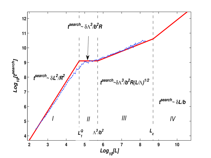
Figure 8:  $t^{search}$ is plotted as a function of $L$, the DNA length for a model with IT and sliding for a quenched DNA. The thin line with dots represent numerical data, while the bold solid line was obtained using Eqs. (33) ,(34), (35) and (36) (see also Fig. 9). In this plot $R$ and $b$ were taken to be $1$ and $20$ lattice constants respectively (the rest of the details could be found in Appendix B). The search time is shown in units of $\delta$.

IV.2 Annealed DNA

Here using the arguments presented in Sec. III.2, the average number of steps performed between two subsequent UITs is of the order of $\frac{1}{p}$ where $p$ is given in Eq. (15). This implies a typical time between the subsequent UITs of the order of $\frac{\delta}{p}$. Using the fact that along the DNA the motion of the protein is diffusive with an effective diffusion constant $D_{1eff}\sim\frac{b^{2}}{\delta}$ one finds

$$\lambda\sim\sqrt{D_{1eff}\frac{\delta}{p}}.$$ (37)

Clearly, $\lambda$ can only take values in the range $b\leq\lambda\leq L$. These with the possible values of $p$ (see Eq. (15)) define the borders of the following three regimes:

• Regime $\mathbf{I}$ occurs for $\lambda\sim L$. Using Eq. (37) and $p=LR^{2}/\Lambda^{3}$ it can be verified that this regime occurs when $L\ll\Lambda\left(\frac{b}{R}\right)^{2/3}$. In this case no UIT occur during the search and Eq. (31) gives

  $$t^{search}\sim\frac{L^{2}}{b^{2}}\delta\;.$$ (38)

• Regime $\mathbf{II}$ occurs when $\Lambda\left(\frac{b}{R}\right)^{2/3}\ll L\ll L_{c}$. Using Eq. (37) and $p=LR^{2}/\Lambda^{3}$ one finds that in this case $\lambda\sim b\sqrt{\frac{\Lambda^{3}}{LR^{2}}}$. Using Eq. (31) gives

  $$t^{search}\sim\frac{\sqrt{\Lambda^{3}L}}{bR}\delta\;.$$ (39)

• Regime $\mathbf{III}$ occurs where $L\gg L_{c}$ and almost all ITs are UITs. Here $\lambda\sim b$ and $p\simeq 1$ so that Eq. (31) gives

  $$t^{search}\sim\frac{L}{b}\delta\;.$$ (40)

The obtained results are summarized in Fig. 9.

One may see that in the case of long sliding, rapid DNA motion cannot decrease the search time significantly as in the pure IT case. This is because long sliding prevents fast decay of correlations.

IV.3 Motion with no CIT

Here we consider a case where the structure of the protein causes it to prefer UITs over CITs. This may occur, for example, in cases where the “legs” of the protein are antiparallel and rigid. The motion on length scale smaller than $\lambda$ is then diffusive involving only sliding with a diffusion coefficient $D_{1}$. In this case, clearly $l_{s}=\lambda$ and the time between two subsequent UITs is given $\frac{\lambda^{2}}{2D_{1}}+\tau_{IT}$ where $\tau_{IT}$ is the time of an UIT. One finds, similar to Sec. II

$$t^{search}\sim\frac{L}{\lambda}\left(\frac{\lambda^{2}}{2D_{1}}+\tau_{IT}\right)\;.$$ (41)

The relationship between this and the picture of Sec. II is given by identifying the antenna’s length $l$ with $\lambda$ and the three-dimensional diffusion time $\tau_{3}$ with $\tau_{IT}$.

Most of the results of Secs. III and IV are summarized in Fig. 9. The results of this section indicate that ITs may supply reasonable search times if they are quick enough. Combining IT with sliding we see that even rare UIT events may break correlations created by one-dimensional diffusion. In this sense ITs act as jumps without the need for detachment from the DNA. Besides this, CITs may effectively accelerate the one-dimensional diffusion or even replace it altogether.

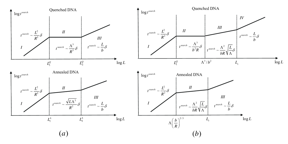
Figure 9:  In this figure the schematic behavior of $t^{search}$ as a function of the DNA length $L$ is shown in absence of the jumps. (a) shows short sliding results ($b\ll R$). (b) shows long sliding results ($b\gg R$).

V Intersegmental transfer and jumping

We now turn to consider the effect of jumping on the results described above. Before addressing the full problem, including ITs sliding and jumping, we first consider a model in which only ITs and jumps occur, and ignore sliding. To include jumping we assign a probability $\frac{dt}{\tau_{1}}$ for a protein to detach from the DNA during a time interval $dt$. The unbinding initiates a jump in which the protein uses three-dimensional diffusion to rebind at a new location on the DNA. Note that since there is no sliding it is safe to assume $b\ll R$.

As argued in the previous section, it is reasonable that both UITs and jumps move the protein to a new location which is chosen randomly on the DNA. Therefore, the search process is composed of a series of one-dimensional scans (occurring through CITs) of the DNA interrupted by uncorrelated relocations. The uncorrelated relocations can occur through two independent processes: jumps and UITs. The typical search time can be evaluated using an approach identical to that of the previous sections.

First, we need to estimate the typical time $\tau_{1eff}$ between two uncorrelated relocations. Combining, the previously derived typical time between two subsequent UITs, $\frac{\lambda^{2}}{2D_{1eff}}$, and the typical time between jumps $\tau_{1}$ we obtain

$$\tau_{1eff}\simeq\frac{1}{\frac{2D_{1eff}}{l^{2}}+\frac{2D_{1eff}}{\lambda^{2}}}\;,$$ (42)

where $\lambda$, defined before, is the typical distance that the protein travels between two subsequent UITs and we define an antenna length $l=\sqrt{2D_{1eff}\tau_{1}}$.

Here and in the next section we focus on the search time as a function of $l$. This quantity is influenced by the protein-DNA non-specific binding energy and governs the frequency of jumps. Other parameters that do not depend on $l$, such as $\lambda$, are taken as fixed. The value of $\lambda$ relevant for the discussion here is given in Sec. III , where $b\ll R$. Note, that when incorporated in the results below the resulting behavior is very complicated. While this is easy to obtain we skip all the regimes and focus on important qualitative behavior.

To proceed we note that the typical distance between two uncorrelated relocation events is given by

$$l_{eff}=\sqrt{2D_{1eff}\tau_{1eff}}\simeq l\sqrt{\frac{1}{1+\frac{l^{2}}{\lambda^{2}}}}\;.$$ (43)

As expected, and seen in Eqs. (42) and (43), the relative importance of both mechanisms is controlled by the ratio $\frac{l}{\lambda}$. In the case of $l/\lambda\gg 1$ jumping is rare compared to UITs and may be neglected leading to the behavior found in Sec. III. In the opposite case $l/\lambda\ll 1$ the possibility of performing an UIT is negligible and the results of Sec. II hold.

Finally, we must estimate the average time spent by the protein performing one uncorrelated relocation. This is given by the average of the jump time, $\tau_{3}$, and the time of an IT, weighed with the probability of performing each. This gives

$$\tau_{3eff} =\tau_{3}\frac{\tau_{1eff}}{\tau_{1}}+\delta\left(1-\frac{\tau_{1eff}}{\tau_{1}}\right)$$

$$=\tau_{3}\frac{l_{eff}^{2}}{l^{2}}+\delta\left(1-\frac{l_{eff}^{2}}{l^{2}}\right)\simeq\frac{\tau_{3}+\delta\frac{l^{2}}{\lambda^{2}}}{1+\frac{l^{2}}{\lambda^{2}}}\;,$$ (44)

where $\frac{1/\tau_{1}}{1/\tau_{eff}}$ is the probability of a jump, $1-\frac{1/\tau_{1}}{1/\tau_{eff}}=\frac{1/\frac{\lambda^{2}}{2D_{1eff}}}{1/\tau_{eff}}$ is the probability of an UIT and $\delta$, defined above is the time of an IT (see Appendix D.2 for a more detailed derivation).

The total search time, as before, takes the form of Eq. (3). Now, each search round is defined as the interval between two subsequent uncorrelated relocations. The total time of one round is $\tau_{r}\sim\tau_{1eff}+\tau_{3eff}$, and therefore the search time is given by

$$t^{search}\sim N_{r}\tau_{r}\sim\frac{L}{l_{s}}\left(\tau_{1eff}+\tau_{3eff}\right)\;.$$ (45)

Here $l_{s}$ is the length scanned between two subsequent uncorrelated relocations. In the case discussed here $b\ll R$, and the value of $l_{s}$ depends on the properties of the search between two uncorrelated relocations, namely the ratio of $l_{eff}$ and $l_{R}$, the recurrence length (see Eq. (10) and the relevant discussion). If $l_{eff}\gg l_{R}$ the search between two subsequent jumps is recurrent and $l_{s}\sim l_{eff}$. However, in the opposite regime, $l\ll l_{R}$, $l_{s}\sim\frac{l_{eff}^{2}}{l_{R}}$.

Therefore, for a given $\lambda$ there are two regimes (see Fig. 10 and 11):

• Regime $\mathbf{I}$ ($l_{R}\ll l_{eff}$):

In this regime, using Eq. (45), the total search time is

$$t^{search} \sim N_{r}\tau_{r}\sim\frac{L}{l_{eff}}\left(\tau_{1eff}+\tau_{3eff}\right)\sim$$

$$\sim\frac{L}{l}\left(\frac{\frac{l^{2}}{2D_{1eff}}+\tau_{3}+\delta\frac{l^{2}}{\lambda^{2}}}{\sqrt{1+\frac{l^{2}}{\lambda^{2}}}}\right)\simeq\frac{L}{l}\frac{\frac{l^{2}}{2D_{1eff}}+\tau_{3}}{\sqrt{1+\frac{l^{2}}{\lambda^{2}}}}\;,$$ (46)

where we used $\lambda\gg R$.

Comparing with Eq. (3) we note that here we have both an effective diffusion constant and an extra  enhancement factor given by $\left(1+\frac{l^{2}}{\lambda^{2}}\right)^{-1/2}$. As we now show, this factor has important consequence.

Consider the value of $\tau_{1}=\frac{l^{2}}{2D_{1eff}}$ for which a minimal search time is obtained and compare it with the usual paradigm of $\left(\tau_{1}^{opt}\right)_{0}=\tau_{3}$. Due to the enhancement factor we now find

$$\tau_{1}^{opt}=\frac{\left(\tau_{1}^{opt}\right)_{0}}{1-\frac{4D_{1eff}\tau_{3}}{\lambda^{2}}}\;,$$ (47)

where $\left(\tau_{1}^{opt}\right)_{0}=\tau_{3}$ (see Eq. (6)) is the optimal antenna size in absence of ITs ($\lambda\rightarrow\infty$) (see Sec. II). It is interesting to note that $l^{opt}$ approaches infinity when $\tau_{3}$ is larger than a critical value

$$\tau_{3c}=\frac{\lambda^{2}}{4D_{1eff}}\;.$$ (48)

Hence, the minimal search time for $\tau_{3}\geq\tau_{3c}$, is identical to that with no jumps (see Sec. III). It is important to note that $\tau_{3c}$ depends, as expected, on the time of an IT through $D_{1eff}$. In the case when $\tau_{3}\leq\tau_{3c}$ Eqs. (46) and (47) give

$$t_{opt}^{search}\sim L\sqrt{\frac{\tau_{3}}{D_{1eff}}}\sqrt{1-\frac{\tau_{3}}{2\tau_{3c}}}\;.$$ (49)

In this regime $t_{opt}^{search}$ is monotonically increasing in $\tau_{3}$.

In Fig. 12 we show a comparison between the results of numerical simulation and Eq. (46).

• Regime $\mathbf{II}$ ($l_{eff}\ll l_{R}$)

In this case $l_{s}\sim\frac{l_{eff}^{2}}{l_{R}}$ and Eq. (45) yields

$$t^{search}\sim\frac{Ll_{R}}{l_{eff}^{2}}\left(\tau_{1eff}+\tau_{3eff}\right)\sim\frac{Ll_{R}}{l^{2}}\left(\frac{l^{2}}{2D_{1eff}}+\tau_{3}\right)\;.$$ (50)

Interestingly, in this regime the minimal search time is obtained when $\tau_{1}$ diverges ; This means that jumping only increase the search slower in this case. We note that some care needs to be taken with the limit since if $\lambda>l_{R}$ and the value of $l$ exceeds $l_{R}$ the regime $l_{eff}\ll l_{R}$ transforms into Regime $\mathbf{I}$.

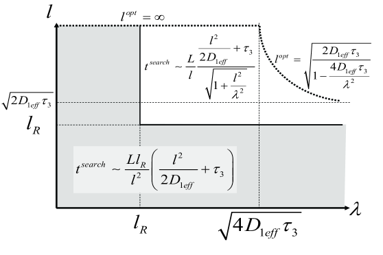
Figure 10: Possible regimes as a function of $l$ and $\lambda$ are shown in the case of ITs and jumping (or IT, jumping and sliding with $b\ll R$) for $l_{R}\ll\sqrt{2D_{1eff}\tau_{3}}$. The gray (white) area represents regime $\mathbf{I}$ ($\mathbf{II}$). The dashed line represents the optimal antenna length. The optimal antenna length in the absence of IT is equal to $\sqrt{2D_{1}\tau_{3}}$.

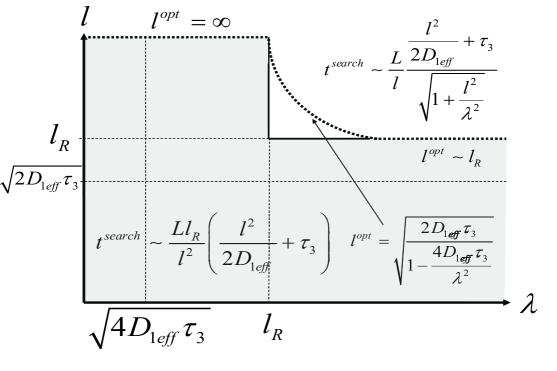
Figure 11: Possible regimes as a function of $l$ and $\lambda$ are shown in the case of ITs and jumping (or IT, jumping and sliding with $b\ll R$) for $l_{R}\gg\sqrt{2D_{1eff}\tau_{3}}$. The gray (white) area represents regime $\mathbf{I}$ ($\mathbf{II}$). The dashed line represents the optimal antenna length. The optimal antenna length in the absence of IT is equal to $\sqrt{2D_{1}\tau_{3}}$.

The results of this section highlight several interesting features which will also appear in the more general case, where sliding is also allowed. First, we note that in the limit of very strong protein-DNA affinity (large values of $\tau_{1}$) the search time becomes robust to changes in the value of $\tau_{1}$. This is very different from a search process with no ITs (see Eqs. (46), (50) and Fig. 12), and may give a possible explanation to the difference between in vitro experiments on the Lac repressor RBC70 . There a strong dependence of the search time on ionic strength (and therefore on the protein-DNA affinity) was found. However, in vivo experiment RCMKAFR87 found that the efficiency of the repression by the same protein is very robust to changes in the ionic strength.

Furthermore, by examining the optimal search time, we find that beyond some critical value of $\tau_{3}$ jumps increase the search time (see Fig. 12 for demonstration). This may give a possible explanation of the obtained value of $\tau_{1}$ in vitro WAC2006 and in vivo ELX2007 for the Lac repressor. These are much larger than the optimal $\tau_{1}$ predicted by models that do not include ITs.

In Fig. 12 a comparison between Eq. (46) and numerical simulation is shown. One may see that increasing the value of $\tau_{3}$ increases the optimal value of $l$ (or equivalently $\tau_{1}$) in such a way that above some critical value, predicted by Eq. (48), it becomes infinite.

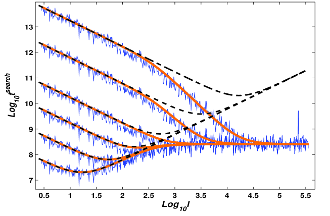
Figure 12: The influence of ITs on the search time is shown.The search time, $t^{search}$, is plotted as a function of the antenna length, $l,$ for a different values of $\tau_{3}$ ($140,\ 1400,\ 14000,\ 1400000,\ 5000000,\ 14000000$ in units of $\delta$ from bottom up). Here only ITs and jumping are allowed. Thin solid lines represent the numerical results. The bold solid lines represent analytic results (Eq. (46)). The black, dashed lines represent the search time in the case with no ITs, obtained by using Eq. (4) with the effective diffusion constant $D_{1eff}=\frac{R^{2}}{2\delta}$ instead of $D_{1}$. Here $L$, $R$ and $b$ were taken to be $1224000$, $1$ and $1$ lattice constants respectively. Since $R=b=1$ diffusion through sliding is identical to one through CITs. This allows us to directly compare sliding and jumping with ITs and jumping.

VI Intersegmental transfer, sliding and jumping

With the results of the previous section it is straightforward to consider the general case where ITs, sliding and jumping are allowed. Similar to the previous section we show that jumping may slow the search process significantly. However, ITs make the search process much more robust to variations in parameters.

First consider the case $b\ll R$ where sliding events are very short. Clearly, in this case the results of the previous section hold with $\delta=\frac{b^{2}}{2D_{1}}+\tau_{IT}$. Here as in Sec. IV, $D_{1}$ is the one dimensional diffusion coefficient for sliding and $\tau_{IT}$ is the typical time that the protein is bound to two DNA segments. With this in mind, in this section we discuss only the opposite case of $b\gg R$. Here, as in Sec. V, the parameters that do not depend on $l$, such as $\lambda$, are taken as given. In Sec. IV contains the relevant derivation of $\lambda$ is calculated for the case discussed here of long sliding, $b\gg R$.

As shown in Sec. IV in this case $D_{1eff}$ $\sim\frac{b^{2}}{2\delta}$ with $\delta=\frac{b^{2}}{2D_{1}}+\tau_{IT}$. Following Sec. V we first need $\tau_{3eff}$, the typical time of an uncorrelated relocation. This is given by (see the derivation of Eq. (44) and Appendix D.1)

$$\tau_{3eff}=\frac{\tau_{3}+\tau_{IT}\frac{l^{2}}{\lambda^{2}}}{1+\frac{l^{2}}{\lambda^{2}}}\;.$$ (51)

Note that here, since $b\gg R$, the search between two subsequent uncorrelated relocations is always recurrent and therefore $l_{s}\sim l_{eff}$. Therefore, similar to Sec. V, the search time is given by

$$t^{search}\sim\frac{L}{l_{eff}}\left(\tau_{1eff}+\tau_{3eff}\right)\sim\frac{L}{l_{eff}}\left(\frac{l_{eff}^{2}}{2D_{1eff}}+\frac{\tau_{3}+\tau_{IT}\frac{l^{2}}{\lambda^{2}}}{1+\frac{l^{2}}{\lambda^{2}}}\right)\;.$$ (52)

Using Eqs. (43) and (52), the total search time can be written as

$$t^{search}\sim\frac{L}{l\sqrt{1+\frac{l^{2}}{\lambda^{2}}}}\left(\frac{l^{2}}{2D_{1eff}}+\tau_{IT}\frac{l^{2}}{\lambda^{2}}+\tau_{3}\right)\;.$$ (53)

Again, it is interesting to consider the optimal value of $\tau_{1}$

$$\tau_{1}^{opt}=\frac{\left(\tau_{1}^{opt}\right)_{0}}{1-\frac{2\tau_{3}-\tau_{IT}}{\lambda^{2}/2D_{1eff}}}\;,$$ (54)

where $\left(\tau_{1}^{opt}\right)_{0}=\tau_{3}$ (see Eq. (6)) is the optimal antenna size in absence of ITs ($\lambda\rightarrow\infty$).

Interestingly, Eq. (54) shows that the optimal $\tau_{1}^{opt}$, may either be smaller or larger than $\left(\tau_{1}^{opt}\right)_{0}$ depending on the time of an IT, $\tau_{IT}$. It is also noteworthy that when $2\tau_{3}>\lambda^{2}/2D_{1eff}+\tau_{IT}$ the optimal $\tau_{1}$ value becomes infinite. Namely, jumping makes the search process slower. This is similar to the behavior found in Sec. V, and again the critical value of $\tau_{3}$ depends on microscopic quantities such as the time of an IT.

The minimal search time obtain is

$$t_{opt}^{search}\sim\left\{\begin{array}[c]{cc}\frac{L}{\lambda}\sqrt{\tau_{3}}\sqrt{\lambda^{2}/2D_{1eff}+\tau_{IT}-\tau_{3}}&\;\;\;\;\;\;\;\tau_{3}<\frac{\lambda^{2}/2D_{1eff}+\tau_{IT}}{2}\\ L\left(\frac{1}{2D_{1eff}}+\frac{\tau_{IT}}{\lambda^{2}}\right)&\;\;\;\;\;\;\;\tau_{3}>\frac{\lambda^{2}/2D_{1eff}+\tau_{IT}}{2}\end{array}\right.\;.$$ (55)

We stress again that it is clearly seen that jumping may slow the search considerably. Note that again the optimal value of $\tau_{1}$ is very different than the canonical one discussed in Sec. II.

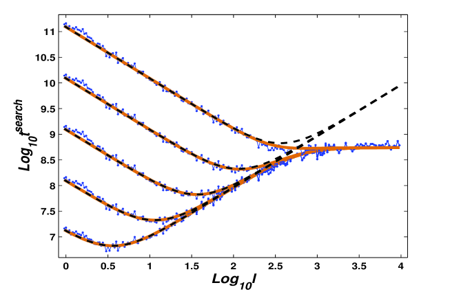
Figure 13: The influence of ITs on the search time is shown. The search time, $t^{search}$, is plotted vs. the antenna length, $l$, for a different values of $\tau_{3}$ ($10,\ 100,\ 1000,\ 10000,\ 100000$ in units of $\delta$ from bottom up). Here ITs, jumping and sliding are allowed. Thin solid lines with dots represent the numerical results. The bold solid lines represent analytic results (Eq. (53)). The black, dashed lines represent the search time in the case with no ITs, obtained by using Eq. (4) with $D_{1eff}=\frac{R^{2}}{2\delta}$. Here $L$, $R$ and $b$ were taken to be $1224000$, $1$ and $20$ lattice constants respectively.

Fig. 13 shows a comparison between the theoretically predicted search time (Eq. (53)) and numerical simulation.

VII Application to the Lac repressor

The above results cover a very wide variety of regimes. For a given protein only several are of interest. To illustrate the use of the results presented above we consider Lac repressor. Lac repressor is both the most studied DNA-binding protein (see M96 for a review) and its structure is highly suggestive of intersegmental transfers taking place. Despite of this several physical parameters of the protein are yet unknown. In this subsection we use the known parameters: $R\sim 10nm$ RR97 , $\Lambda\sim 1\mu$, $L\sim 1mm$, and those measured for Lac repressor with only one DNA-binding domain $\tau_{1}\sim 1ms$, $\tau_{3}\sim 0.1\tau_{1}$ and $D_{1}\sim 0.05\mu^{2}/s$ WAC2006 ; ELX2007 . Still unknown are $b$, the sliding length, and $\tau_{IT}$ which we use as free parameters and study the search time as these are varied. It is interesting to note that Lac repressor is so large that, as we show, essentially all ITs can move the protein at each step to a completely uncorrelated location on the DNA.

Fig. 14 shows the predicted $t^{search}$ from Secs. V and VI as a function of $b$ and $\tau_{IT}$. One may see that for $b\gg R$, ITs do not affect the search time significantly even if $\tau_{IT}$ is small. This is results from the small probability of performing UIT for a large values of $b$. However, if $b\ll R$ the search time may be decreased in a significant manner by including ITs. For example, by setting $b$ to be the size of one base pair $\sim 0.3nm$ the search time decrease by a factor of three when $\tau_{IT}=\tau_{3}$ and if $\tau_{IT}=\frac{\tau_{3}}{10}$ the search time decreases by a factor of ten. Finally, Fig. 14 shows that for large values of $\tau_{IT}$, ITs may slow down the search process.

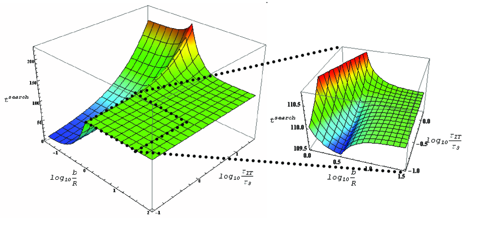
Figure 14: On this figure the analytical prediction of $t^{search}$ is shown as a function of the unknown parameters $b$ and $\tau_{IT}$.

VIII Summary

In this article we presented a comprehensive study of the influence of ITs on the search process. Using simple scaling arguments we studied a model which includes the protein dynamics and DNA conformation. Two extreme regimes for the DNA dynamics were studied: completely quenched (frozen) and annealed (rapidly moving) DNA. ITs were assumed to relocate the protein to a randomly chosen DNA position within a range of the order of the protein size. The essence of the description may be understood from Sec. III. The following sections elaborate and study a search processes based on ITs with sliding and/or jumping. The results for a particular protein of interest may be obtained by suitably selecting the section most relevant for a particular case.

The obtained results clearly indicate that including IT in the search process may increase, the robustness of the search efficiency to different parameters of the model such as the protein-DNA affinity, the three-dimensional diffusion coefficient etc.

The mechanism of IT may produce a significant increase of the optimal residence time of the protein on the DNA between two subsequent rounds of three-dimensional diffusion from the value predicted by the models that do not include IT. Recent experiments indicates that the value of the residence time of the proteins on the DNA between two subsequent rounds of the three-dimensional diffusion is much larger than the optimum predicted by the model. It is possible that the existence of the IT mechanism may explain the rather quick search times found in vivo experiments.

One of the most surprising results found that above some critical value of the typical time of a jump the protein has no reason to detach from the DNA. It is more efficient for it to stay bound to the DNA. The value of the critical jump time depends on the time of an IT.

A key ingredient needed for the behavior to occur is the confinement of the DNA in a volume much smaller than its radius of gyration. The probability to perform an UIT obviously depends on the DNA density. Larger density implies a larger probability for UITs. Therefore the effects of IT are expected to be more important in the systems with high DNA density as cells or eucaryotic nuclei rather than in the in vitro experiments.

The dependency, mentioned above, on the DNA density leads to many possible regimes which depend on the cell size, DNA length etc. In particular, we found non-trivial regimes when the search time increases as a square root of the DNA length or is completely independent of it. Our estimates indicate that these seem to be the ones most relevant to experiments.

Our results also show that the search on quenched and annealed DNA may have quite different scaling behavior. In general a search that uses ITs is shown to be more rapid on an annealed DNA than on a quenched DNA. This happens due to the rapid decrease in correlations which results from the motion of the DNA molecule.

Similar scaling arguments were used to discuss the effects of IT in HS2007 . However, there the main mechanism that drives the IT was assumed to be the motion of the DNA molecule. In our study even on completely quenched DNA ITs are shown to be important.

Appendix A

In this appendix we argue that the typical time that the protein spends in a jump is given by $\tau_{3}\sim\frac{\Lambda^{3}}{D_{3}L}$. This quantity is controlled by average volume which is free from DNA. Consider, first, the probability to find a volume, free from DNA of radius $s$. To do so we describe the packed DNA as an ideal gas of $\frac{L}{L_{0}}$ straight rods of length $L_{0}$ that are distributed randomly in the cell (see Fig. 3). The probability $p_{seg}$, that a given rods crosses a volume of radius $s$ is of order of $\frac{L_{0}^{3}}{\Lambda^{3}}\frac{s^{2}}{L_{0}^{2}}=\frac{L_{0}s^{2}}{\Lambda^{3}}$. Here $\frac{L_{0}^{3}}{\Lambda^{3}}$ is the probability that a given segments is located within a distance $L_{0}$ of a point inside the cell and $\sim\frac{s^{2}}{L_{0}^{2}}$ is the probability that this segment crosses a sphere of radius $s$ around the point. The probability that at least one segment crosses the void is

$$1-\left(1-p_{seg}\right)^{L/L_{0}}\simeq 1-e^{-\frac{LR^{2}}{\Lambda^{3}}}\;.$$ (56)

Therefore the typical free volume radius is $\sim\sqrt{\frac{\Lambda^{3}}{L}}$. Hence, the typical time to explore this volume is $\tau_{3}\sim\frac{\Lambda^{3}}{D_{3}L}$. A second way to get the same expression for $\tau_{3}$ is based on a comparison between Eqs. (1) and (4). Obviously, in the limiting case $\tau_{1}\ll\tau_{3}$ and $\sqrt{2D_{1}\tau_{1}}=r$, the search becomes based only on the three-dimensional diffusion. Hence, in this case the formula (4) should give (1). It is easy to see that this happens only when $\tau_{3}\sim\frac{\Lambda^{3}}{D_{3}L}$.

Appendix B

In this appendix we describe the details of the numerical simulation. The simulations were done on a cubic lattice containing $800\times 800\times 800$ sites. Assuming that a real cell has a volume of $1\mu m^{3}$ each site on the lattice represents a volume of $\left(dx\right)^{3}=\left(\frac{\mu m}{800}\right)^{3}$. Polymers (representing the DNA) with different lengths were embedded in the lattice by using a self-avoiding random walk. The persistence length was accounted for by assigning a probability $p_{0}$ of changing direction randomly among the possible directions. Using the persistence length of about $50nm$ leads to $p_{0}=\frac{dx}{50nm}=0.025$. If during the process of generating the configuration the polymer length can not be extended we shrink the polymer by $O\left(10\right)$ lattice constants and regenerate. While this leads to a bias in the configuration for single realization confined in a box, which are of interest, we expect no effect on the results (a non biased algorithm is not plausible within our computational resources). The search process is simulated following the model described in the text. In each step the protein has a probability $\frac{dx^{2}}{2b^{2}}$ to perform an IT and a probability $\frac{dx^{2}}{2l^{2}}$ to perform a jump. ITs were simulated by a randomly choosing a DNA site within a distance $R$ from the location of the protein. With the exception of Sec. II, where a complete simulation of the three-dimensional diffusion was carried out by performing moves to the $6$ available directions, a jump was simulated by randomly choosing a site on the DNA. The time of the jump was taken as a free constant ().

Appendix C

In this appendix we argue that using ITs the protein can only move along the chemical coordinate to distances smaller than $R$ or larger than $\frac{\Lambda^{2}}{L_{0}}$. As mentioned above, we assume that during an IT the protein chooses a new location whose three-dimensional distance from its current location is smaller than $R$. The new location is chosen randomly with a uniform probability. Given the uniform probability we need to estimate the total typical length available at each IT, $G$. We separate  this quantity to four types of contributions:

$$G=G_{1}+G_{2}+G_{3}+G_{4}\;.$$ (57)

The first $G_{1}$ is the contribution from DNA whose distance along the chemical coordinate from a point $x$ is smaller than $R$, the protein size. This is given by

$$G_{1}\left(x\right)\simeq 2R\;.$$ (58)

The contribution $G_{2}$ arises from DNA whose chemical distance from a point $x$ is larger than $R$ but smaller than $L_{0}$. The probability for the DNA to bend on a scale $l$ is approximately given by $\frac{1-e^{-l/2L_{0}}}{L_{0}}$. However, the probability that this bend will connect to $x$ is $\sim\frac{R^{2}}{l^{2}}$ (due to the area ratio). Since each connection contributes a length of the order of$\ R$ to $G_{2}$ we obtain

$$G_{2}\sim R{\int\limits_{R}^{L_{0}}}\frac{1-e^{-l/2L_{0}}}{L_{0}}\frac{R^{2}}{l^{2}}dl\sim\frac{R^{2}}{L_{0}}\left(1-e^{-R/2L_{0}}\right)\simeq\frac{R^{3}}{L_{0}^{2}}\;.$$ (59)

The contribution $G_{3}$ comes from DNA whose chemical distance from $x$ is larger than $L_{0}$ but smaller than the length at which the DNA feels the boundaries of the cell is $\sim\frac{\Lambda^{2}}{L_{0}}$. This value can be overestimated using the fact that a free three-dimensional random walk on a lattice returns to the origin about $1.5$ times on average. Therefore, a continuous free three-dimensional random walk with persistence length $L_{0}$ returns to a region with radius $R$ an order of $\left(\frac{R}{L_{0}}\right)^{2}$ times. Each such return contributes length of about $R$ to $G_{3}$, leading to

$$G_{3}\sim\frac{R^{3}}{L_{0}^{2}}\;.$$ (60)

Finally, $G_{4}$ is the contribution from the rest of the DNA (whose chemical distance is larger than $\frac{\Lambda^{2}}{L_{0}}$ but smaller than $L$). Using (13) and since each connected segment contributes a length of the order $R$ to $G_{4}$ one obtains

$$G_{4}\sim R\frac{L}{L_{0}}p_{seg}\sim\frac{LR^{3}}{\Lambda^{3}}\;.$$ (61)

This result can be understood within a mean field approach: if the DNA has a total length $L$ and is assumed to be distributed uniformly in the cell, every volume in the cell contains a part of the total DNA length that is equal to the total DNA length times the fraction of the volume. One can see that in the assumed regime where $L_{0}\gg R$ and $L\gg\Lambda\frac{\Lambda^{2}}{L_{0}^{2}}$, $G_{2}$ and $G_{3}$ are much smaller than $G_{4}$ and $G_{1}$. Therefore, we can safely neglect the probability that the protein will move to a location on the DNA whose chemical distance from protein’s actual location is larger than $R$ and smaller than $\frac{\Lambda^{2}}{L_{0}}$.

Appendix D

In this appendix the effective times $\tau_{1eff}$ and $\tau_{3eff}$ are calculated.

D.1 The effective time of a correlated movement

We have two independent mechanisms for an uncorrelated motion. The first is jumping with a typical time of $\tau_{1}$ between two subsequent jumps. This process has Poissonian statistics and therefore the probability that the protein does not perform a jump before time $t$ is

$$P_{J}=\exp\left(-\frac{t}{\tau_{1}}\right)\;.$$ (62)

The second mechanism for uncorrelated motion is an UIT with a typical time of order of $\frac{\lambda^{2}}{D_{1eff}}$ between two subsequent UITs. In the case of annealed DNA this mechanism has Poissonian statistics and the probability that the protein does not perform an UIT before time $t$ is

$$P_{IT}\sim\exp\left(-\frac{t}{\lambda^{2}/D_{1eff}}\right)\;.$$ (63)

For quenched DNA the probability that the protein did not performed an UIT after traveling distance $x$ is $\sim e^{-x/\lambda}$. Since the protein performs an effective one-dimensional diffusion, $x\sim\sqrt{2D_{1eff}t}$ and we obtain

$$P_{IT}\sim\exp\left(-\sqrt{\frac{t}{\lambda^{2}/2D_{1eff}}}\right)\;.$$

We will take the typical time of a non-interrupted (by an uncorrelated relocation) one-dimensional effective diffusion to be

$$\tau_{1eff}=\int_{0}^{\infty}P_{IT}P_{J}dt\sim\frac{1}{2}\frac{1}{\frac{D_{1eff}}{l^{2}}+\frac{D_{1eff}}{\lambda^{2}}}\;.$$ (64)

The last expression is exact in the annealed case but it is only an approximation in the quenched regime. One can verify that the error does not exceed $50\%$, which is sufficient for scaling arguments of the type used in the paper.

D.2 The effective time of an uncorrelated movement

Since there are two mechanisms for uncorrelated movement: a jump with a typical time $\tau_{3}$ and an UIT with a typical time $\delta$ the typical time of the uncorrelated movement is the average of $\tau_{3}$ and $\delta$ weighted by the relevant probabilities for each process:

$$\tau_{3eff} =\delta\int_{0}^{\infty}\left(-\frac{dP_{IT}}{dt}\right)P_{J}dt+\tau_{3}\int_{0}^{\infty}\left(-\frac{dP_{J}}{dt}\right)P_{IT}dt=$$

$$=\delta\int_{0}^{\infty}\frac{dP_{J}}{dt}P_{IT}dt-\tau_{3}\int_{0}^{\infty}\frac{dP_{J}}{dt}P_{IT}dt-\delta\int_{0}^{\infty}\frac{d}{dt}\left(P_{J}P_{IT}\right)dt=$$

$$=\frac{\tau_{3}-\delta}{\tau_{1}}\int_{0}^{\infty}P_{J}P_{IT}dt+\delta=\frac{\tau_{3}-\delta}{\tau_{1}}\tau_{1eff}+\delta=$$

$$=\tau_{3}\frac{\tau_{1eff}}{\tau_{1}}+\delta\left(1-\frac{\tau_{1eff}}{\tau_{1}}\right)=\tau_{3}\frac{l_{eff}^{2}}{l^{2}}+\delta\left(1-\frac{l_{eff}^{2}}{l^{2}}\right)=\frac{\tau_{3}+\delta\frac{l^{2}}{\lambda^{2}}}{1+\frac{l^{2}}{\lambda^{2}}}\;.$$ (65)

In the case of sliding $\delta$ is replaced by $\tau_{IT}$.

References

- [1] B. Alberts, D. Bray, J. Lewis, M. Raff, K. Roberts, and J. D. Watson. The molecular biology of the cell. Garland, New York, 4’th edition, 1994.
- [2] C. Loverdo, O. Benichou, M. Moreau, and R. Voituriez. Enhanced reaction kinetics in biological cells. Nature Physics, 4:134, 2007.
- [3] M. von Smoluchowski. Mathematical theory of the kinetics of the coagulation of colloidal solutions. Z. Phys. Chem., 92:129, 1917.
- [4] M. B. Elowitz, M. G. Surette, P. E. Wolf, J. B. Stock, and S. Leibler. Protein mobility in the cytoplasm of Escherichia coli. J. Bacteriol., 181(1):197, 1999.
- [5] S. Y. Lin and A. D. Riggs. Lac repressor binding to non-operator DNA: detailed studies and a comparison of eequilibrium and rate competition methods. J. Mol. Biol., 72(3):671, 1972.
- [6] A. D. Riggs, H. Suzuki, and S. Bourgeois. Lac repressor-operator interaction I. Equilibrium studies. J. Mol. Biol., 48(1):67, 1970.
- [7] A. D. Riggs, S. Bourgeois, and M. Cohn. The Lac repressor-operator interaction. 3. Kinetic studies. J. Mol. Biol., 53(3):401, 1970.
- [8] O. G. Berg, R. B. Winter, and P. H. von Hippel. Diffusion-driven mechanisms of protein translocation on nucleic acids. 1. models and theory. Biochemistry, 20(24):6929, 1981.
- [9] M. Slutsky and L. A. Mirny. Kinetics of protein-DNA interaction: Facilitated target location in sequence-dependent potential. Biophys J., 87:4021, 2004.
- [10] T. Hu, A. Y. Grosberg, and B. I. Shklovskii. How proteins search for their specific sites on DNA: The role of DNA conformation. Biophys J., 90:2731, 2006.
- [11] Tao Hu and B. I. Shklovskii. How proteins search for their specific sites on DNA: The role of intersegment transfer. Phys. Rev. E, 76:051909, 2007.
- [12] O. G. Berg and C. Blomberg. Association kinetics with coupled diffusional flows. special application to the Lac repressor-operator system. Biophys. Chem., 4:367, 1976.
- [13] S. E. Halford and J. F. Marko. How do site-specific DNA-binding proteins find their targets? Nucleic Acids Research, 32(10):3040, 2004.
- [14] B.P. Belotserkovskii and D.A. Zarling. Analysis of a one-dimensional random walk with irreversible losses at each step: applications for protein movement on DNA. J. Theor. Biol., 226:195, 2004.
- [15] H. X. Zhou. A model for the mediation of processivity of DNA-targeting proteins by nonspecific binding: Dependence on DNA length and presence of obstacles. Biophysical Journal, 88:1608, 2005.
- [16] M. A. Lomholt, T. Ambjrnsson, and R. Metzler. Optimal target search on a fast-folding polymer chain with volume exchange. Phys. Rev. Lett., 95:260603, 2005.
- [17] G. Adam and M. Delbruck. Reduction of dimensionality in biological diffusion processes. In A. Rich and N. Davidson, editors, Structural Chemistry and Molecular Biology, pages 198–215, San Francisco, CA, 1968. Freeman.
- [18] B. D. Hughes. Random walks and random enviroments, volume 1: Random walks. Clarendon press, Oxford, UK, 1995.
- [19] Y. M. Wang, Robert H. Austin, and Edvard C. Cox. Single molecule measurement of repressor protein 1d diffusion on DNA. Phys.Rev. Lett., 97:048302, 2006.
- [20] J. Elf, G.-W. Li, and P. X. Xie. Probing transcription factor dynamics at the simple single-molecule level in a living cell. Science, 316:1191, 2007.
- [21] Y. Kao-Huang, A. Revzin, A. P. Butler, P. O’Conner, D. W. Noble, and P. H. Von Hippel. Nonspecific DNA binding of genome-regulating proteins as a biological control mechanism: Measurement of DNA-bound Escherichia coli Lac repressor in vivo. PNAS, 74:4228, 1977.
- [22] P. H. von Hippel, A. Revzin, C. A. Gross, and A. C. Wang. In H. Sund and G. Blauer, editors, Protein-Ligand Interactions, pages 279–347, Berlin, 1975. Walter de Gruyter.
- [23] J. L. Bresloff and D. M. Crothers. DNA-ethidium reaction kinetics: demonstration of direct ligand transfer between DNA binding sites. L. Mol. Biol., 172:263, 1975.
- [24] R. Fickert and B. Muller-Hill. How Lac repressor finds Lac operator in vitro. J. Mol. Biol., 226(1):59, 1992.
- [25] T. Ruusala and D. M. Crothers. Sliding and intermolecular transfer of the Lac repressor: Kinetic perturbation of a reaction intermediate by a distant DNA sequence. Proc. Natl. Acad. Sci. USA, 89:4903, 1992.
- [26] B. A. Lieberman and S. K. Nordeen. DNA intersegment transfer, how steroid receptors search for a target site. J. Biol. Chem., 272(2):1061, 1997.
- [27] M. L. Embleton, S. A. Williams, M. A. Watson, and S. E. Halford. Specificity from the synapsis of DNA elements by the SfiI endonuclease. J. Mol. Biol., 289(4):785, 1999.
- [28] C. Bustamante, M. Guthold, X. Zhu, and G. Yang. Facilitated target location on DNA by individual Escherichia coli RNA polymerase molecules observed with the scanning force microscope operating in liquid. ASBMB, 274(24):16665, 1999.
- [29] M. G. Fried and D. M. Crothers. Kinetics and mechanism in the reaction of gene regulatory proteins with DNA. J. Mol. Biol., 172:263, 1984.
- [30] S. Condamin, O. Be nichou, V. Tejedor, R. Voituriez, and J. Klafter. First-passage times in complex scale-invariant media. Nature, 450:77, 2007.
- [31] S. Y. Lin and A. D. Riggs. The general affinity of Lac repressor for E. coli DNA: implication for gene regulation in procaryotes and eucaryotes. Cell, 4:107, 1975.
- [32] B. Richey, D. S. Cayley, M. C. Mossing, C. Kolka, C. F. Anderson, T. C. Farrar, and M. T. Record. Variability of the intracellular ionic environment of Escherichia coli. differences between in vitro and in vivo effects of ion concentrations on protein-DNA interactions and gene expression. J. Biol. Chem, 262:7157, 1987.
- [33] D. J. Watts. Small Worlds: The Dynamics of Networks Between Order and Randomness. Princeton University Press, 1999.
- [34] M. Muller-Hill. The Lac operon. A short history of a genetic paradigm. Walter de Gruyter, Berlin, 1996.
- [35] G. C. Ruben and T. B. Roos. Conformation of Lac repressor tetramer in solution, bound and unbound to operator DNA. Microscopy Research and Technique, 36:400, 1997.