Waiting time models of cancer progression

Abstract

Cancer progression is an evolutionary process that is driven by mutation and selection in a population of tumor cells. We discuss mathematical models of cancer progression, starting from traditional multistage theory. Each stage is associated with the occurrence of genetic alterations and their fixation in the population. We describe the accumulation of mutations using conjunctive Bayesian networks, an exponential family of waiting time models in which the occurrence of mutations is constrained to a partial temporal order. Two opposing limit cases arise if mutations either follow a linear order or occur independently. We derive exact analytical expressions for the waiting time until a specific number of mutations have accumulated in these limit cases as well as for the general conjunctive Bayesian network. Finally, we analyze a stochastic population genetics model that explicitly accounts for mutation and selection. In this model, waves of clonal expansions sweep through the population at equidistant intervals. We present an approximate analytical expression for the waiting time in this model and compare it to the results obtained for the conjunctive Bayesian networks.
Keywords: Bayesian network, cancer, genetic progression, multistage theory, Wright-Fisher process

I Introduction

Cancer is a genetic disease that develops as the result of mutations in specific genes. When these genes work normally, they control the growth of cells in the body. Cancer cells have lost the normal cooperative behavior of cells in multicellular organisms resulting in increased proliferation. Tumor development starts from a single genetically altered cell and proceeds by successive clonal expansions of cells that have acquired additional advantageous mutations. The progression of cancer is characterized by the accumulation of these genetic changes (Cairns, 1975; Nowell, 1976; Merlo et al., 2006; Michor et al., 2004; Crespi and Summers, 2005).

Many oncogenes and tumor suppressor genes have been identified that contribute to tumorigenesis (Futreal et al., 2004). In general, the mutational patterns of cancer cells vary greatly, not only among cancer types, but also among individual tumors of the same type. Some of this genetic variation might be due to the fact that all cancer cells need to acquire certain functional changes, the hallmarks of cancer, and most of these functions are accomplished by several gene products acting together in signaling pathways (Hanahan and Weinberg, 2000; Vogelstein and Kinzler, 2004). Thus, many different genetic alterations can have similar phenotypic effects.

The incidence of sporadic cancer indicates that the underlying events are stochastic and that, in general, several steps are necessary. Therefore, a random processes approach appears to be an appropriate modeling strategy. The progression stages are generally not observable on a molecular level in vivo, and in a clinical setting, patients are typically diagnosed at the final stages of tumorigenesis. Mathematical modeling plays an important role in cancer research today, because it can be used to reconstruct and to analyze the evolutionary process driving cancer progression (Anderson and Quaranta, 2008).

Models of tumorigenesis have been proposed early on to explain cancer incidence data (Nordling, 1953; Armitage and Doll, 1954; Knudson, 1971). These models assume that cancer is a stochastic multistep process with small transition rates and they have been further developed into the multistage theory of cancer (Moolgavkar and Luebeck, 1992; Frank, 2007; Jones et al., 2008a). The tumor stages may be defined by specific mutations, by the number of mutations, by epigenetic changes, by functional alterations, or by histological properties. Since cancer progression is an evolutionary process, population genetics models are used extensively to describe tumorigenesis (Nowak, 2006; Wodarz and Komarova, 2005; Schinazi, 2006; Beerenwinkel et al., 2007a; Durrett et al., 2008). Various deterministic and stochastic models have been proposed, some of which address specific questions, such as the dynamics of tumor suppressor genes (Iwasa et al., 2005), genetic instability (Nowak et al., 2006), or tissue architecture (Nowak et al., 2003).

As more and more genetic data from cancer cells become available from comprehensive studies (Sjöblom et al., 2006; Wood et al., 2007; Jones et al., 2008b; Parsons et al., 2008; Ley et al., 2008) and through databases (Futreal et al., 2004; Baudis, 2007; Mitelman et al., 2008), one can also start investigating the dependencies between genetic events using statistical models. In view of multistage theory, tumors proceed through distinct stages, which can be characterized by the appearance of certain mutations. Particular attention has been paid to inferring the order of genetic alterations. Several graphical models have been developed for this purpose and applied to various cancer types (Desper et al., 1999; Radmacher et al., 2001; Hjelm et al., 2006; Rahnenführer et al., 2005; Beerenwinkel et al., 2006, 2007b; Beerenwinkel and Sullivant, 2008).

A quantitative understanding of carcinogenesis can help developing new diagnostic and prognostic markers. Today a variety of univariate genetic markers is known (Sidransky, 2002), most of them comprising well-known oncogenes or tumor suppressors. Because of the diverse genetic nature of cancer, markers measuring the accumulation of several mutations, i.e., the progression of cancer, may improve existing ones. Here, we investigate the dynamics of cancer progression as a function of transition rates and of order constraints on the genetic events. The expected waiting time can be regarded as a measure of genetic progression to cancer (Rahnenführer et al., 2005).

In Section II, we introduce the general stochastic multistep process and present an equivalent description in terms of ordinary differential equations (ODEs). At this abstract level of description, carcinogenesis may be regarded as proceeding through distinct stages, which can be defined by histological grades, functional changes, or genetic alterations. In Section III, these stages will be associated with the occurrence of a certain number of mutations. We present expressions of the waiting time until a given stage is reached, for different models of mutation. Finally, in Section IV, we analyze an evolutionary model of carcinogenesis explicitly describing the appearance of genetic alterations in the tissue by mutations in single cells and their subsequent clonal expansions.

II Multistage theory

The multistage theory of cancer postulates that tumorigenesis is a linear multistep process, in which each step from one stage to the next is a rare event (Figure 1). Let us denote the cancer stages by $0$, $1$, $2$, $\dots$, $k$, where stage $0$ refers to the normal precancerous state, $1$ to the first adenomatous stage, and $k$ to a defined cancerous endpoint, such as the the formation of metastases. The process is started at time $t=0$ in state $0$.

Figure 1: The multistage model. Cancer is assumed to develop in a linear process consisting of $k$ stages. The progression steps mark the major transitions of the tissue from normal to cancerous and eventually to metastasizing. At each transitions $(j-1)\to j$ the waiting time follows an exponential distribution with parameter $u_{j}$ giving rise to the model defined by Eq. (1).

The transition rate from stage $j-1$ to stage $j$ is denoted $u_{j}$. That is, the waiting times for the transitions to occur are assumed to be independently exponentially distributed. Here, the coefficients $u_{j}$ denote the transition rates between the stages of tumor development; later we will link them to different models of mutation and fixation. Because of the sequential nature of the linear model, the waiting time $\tau_{k}$ until stage $k$ is reached is given recursively by the sum of exponentially distributed random variables,

$$\tau_{1}\sim\operatorname{Exp}(u_{1}),\qquad\tau_{j}\sim\tau_{j-1}+\operatorname{Exp}(u_{j}),\quad j=2,\dots,k.$$ (1)

The waiting times follow the linear order $\tau_{1}<\dots<\tau_{k}$ and the expected waiting time is

$$\mathbb{E}[\tau_{k}]=\mathbb{E}[\tau_{k-1}]+\frac{1}{u_{k}}=\sum_{j=1}^{k}\frac{1}{u_{j}}.$$ (2)

In particular, if all transition rates are equal, $u_{j}=u$ for all $j=1,\dots,k$, we find $\mathbb{E}[\tau_{k}]=k/u$. Hence the waiting time scales linear in the number of transitions $k$.

Let $f_{\tau_{1},\dots,\tau_{k}}(t_{1},\dots,t_{k})$ be the density function of the joint distribution of waiting times $\tau=(\tau_{1},\dots,\tau_{k})$ defined by Eq. (1). The linear order of the waiting times $\tau_{j}$ induces the factorization

$$f_{\tau_{1},\dots,\tau_{k}}(t_{1},\dots,t_{k})=\prod_{j=1}^{k}f_{\tau_{j}|\tau_{j-1}}(t_{j}\mid t_{j-1})$$ (3)

of $f_{\tau_{1},\dots,\tau_{k}}$ into the conditional densities

$$\begin{split}f_{\tau_{j}|\tau_{j-1}}(t_{j}\mid t_{j-1})=u_{j}\exp\left(-u_{j}[t_{j}-t_{j-1}]\right)\,\mathbb{I}(t_{j}>t_{j-1}),\end{split}$$ (4)

where $\mathbb{I}$ is the indicator function.

Multistage theory can also be formulated as a system of ordinary differential equations (ODEs). We derive this formulation as follows: Let $x_{j}(t)$ denote the probability that stage $j$ is reached before time $t\geq 0$, but stage $j+1$ has not yet been reached,

$$x_{0}(t) = \operatorname{Prob}[0<t<\tau_{1}]$$

$$x_{j}(t) = \operatorname{Prob}[\tau_{j}<t<\tau_{j+1}],\quad j=1,\dots k-1,$$ (5)

$$x_{k}(t) = \operatorname{Prob}[\tau_{k}<t].$$

We have $x_{0}(t)+\dots+x_{k}(t)=1$ and $x_{j}(t)=\operatorname{Prob}[t<\tau_{j+1}]-\operatorname{Prob}[t<\tau_{j}]$ due to the linearity of transitions. It follows that $\dot{x}_{j}(t)=f_{\tau_{j+1}}(t)-f_{\tau_{j}}(t)$.Using the conditional exponential nature of the model, Eq. (4), one finds that $f_{\tau_{j}}(t)=\int_{0}^{\infty}f_{\tau_{j},\tau_{j-1}}(t,t^{\prime})\,\mathrm{d}t^{\prime}=\int_{0}^{t}\exp(-u_{j}[t-t^{\prime}])f_{\tau_{j-1}}(t^{\prime})\,\mathrm{d}t^{\prime}$. From the identity $\exp(-u_{j}t)=u_{j}\int_{t}^{\infty}\exp(-u_{j}t^{\prime})\,\mathrm{d}t^{\prime}$, one obtains

$$f_{\tau_{j}}(t) =u_{j}\int_{t}^{\infty}\!\!\!\int_{0}^{t}\exp(-u_{j}[t^{\prime\prime}-t^{\prime}])f_{\tau_{j-1}}(t^{\prime})\,\mathrm{d}t^{\prime}\,\mathrm{d}t^{\prime\prime}$$

$$=u_{j}\int_{t}^{\infty}\!\!\!\int_{0}^{t}f_{\tau_{j},\tau_{j-1}}(t^{\prime\prime},t^{\prime})\,\mathrm{d}t^{\prime}\,\mathrm{d}t^{\prime\prime}$$ (6)

$$=u_{j}\operatorname{Prob}[\tau_{j-1}<t<\tau_{j}]=u_{j}x_{j-1}(t).$$

Hence, the probabilities $x_{j}(t)$ obey the set of ODEs,

$$\dot{x}_{0}(t) = -u_{1}\,x_{0}(t),$$

$$\dot{x}_{j}(t) = u_{j}x_{j-1}(t)-u_{j+1}x_{j}(t),\quad j=1,\dots,k-1,\quad$$ (7)

$$\dot{x}_{k}(t) = u_{k}\,x_{k-1}(t),$$

subject to initial conditions $x_{0}(0)=1$ and $x_{j}(0)=0$ for all $j\geq 1$. These rate equations describe the linear chain of exponential waiting time processes as a probability flux of rate $u_{j}x_{j-1}(t)$ from state $j-1$ to state $j$.

If all rates are identical, $u_{j}=u$ for all $j$, then the solution of this linear system of ODEs is given by Poisson distributions with time-dependent parameter $ut$,

$$x_{j}(t)=\operatorname{Pois}(j;ut)=\frac{(ut)^{j}\exp(-ut)}{j!},\quad j=0,\dots,k-1.$$ (8)

The probability of having reached the final stage of progression, $k$, at time $t$ is

$$x_{k}(t)=1-e^{-ut}\,\sum_{j=0}^{k-1}\frac{(ut)^{j}}{j!}=\operatorname{Pois}(k;ut)\sum_{j=0}^{\infty}\frac{(ut)^{j}}{(k+j)_{j}}.$$ (9)

We also recover from the ODE system the expected waiting time to the final cancer stage,

$$\mathbb{E}[\tau_{k}]=\int_{0}^{\infty}utx_{k-1}(t)\,\mathrm{d}t=\frac{k}{u}.$$ (10)

Multistage theory provides a mathematical framework for describing the stepwise progression of cancer. For the above discussion of the model, we have neither specified the definition of the postulated stages, nor the nature of the transitions. Indeed, different interpretations and uses of the model are possible. In the following we link multistage theory closely to the genetic progression of cancer.

III Genetic progression of cancer

In this section, we associate the stages of tumorigenesis to mutations in the genomes of cancer cells. Each stage is defined by the number of mutations that have accumulated in the cells of the tissue. Each mutation occurs initially in a single cell as the result of an erroneous DNA duplication. Some mutations alter the behavior of the cell in such a way that it experiences a growth advantage relative to the other cells in the tissue. These cells can outgrow their competitors in a clonal expansion and the mutation spreads in the tissue. While the first appearance of a mutation is essentially a random process, i.e., each mutation is equally likely to appear, the fate of a mutation in the population depends on the relative fitness of the cell in which it occurs.

We define tumor progression to be in stage $j$ of the multistep model, Eq. (1), if most of the tumor cells harbor exactly $j$ mutations. We are interested in the waiting time until $k$ out of $d$ possible mutations have accumulated, where typically $k\ll d$. For example, Sjöblom et al. (2006) suggest that $k\approx 20$ genes out of $d\approx 100$ to $1000$ need to be hit in order to develop invasive colon cancer. In this interpretation of multistage theory, stages correspond to population states and transitions correspond to genetic transformations of the ensemble of tumor cells, including mutation and selection. These population dynamics will be investigated in more detail in the next section. The focus of the present section is on how different models of accumulating mutations affect the waiting time.

Genetic mutations occur randomly at erroneous cell divisions, but the subsequent fixation of the mutation within the cell population is constrained: A mutation will only spread if it confers a growth advantage. This restricts not only the mutations driving cancer, but also the order in which they can appear, because some physiological changes must be achieved before others. For example, in colon cancer, cells must lose the ability to undergo apoptosis, before additional mutations accumulate in the resulting neoplasia. Hence loss of function of the tumor suppressor gene APC controlling apoptosis is necessary before other mutations such as KRAS2 can fixate (Nowak et al., 2003; Vogelstein and Kinzler, 2004). Furthermore, sometimes only the combined action of mutations drives cancer progression. It is known, for example, that only the combination of p53 and Ras trigger the development of tumors in mice (Land et al., 1983).

In general, there may exist several order constraints for the successive fixation of mutations as shown in Figure 2. The simplest of these constraints is the linear model, where the waiting times of all mutations are totally ordered (Figure 2(a)). The linear model is exactly the multistep process discussed in the previous section. Alternatively, mutations may occur independently without any constraints (Figure 2(b)). If there exist order relations among some of the possible mutations, a partial order may be used to describe the process of accumulating mutations (Figure 2(c)). We will discuss these models separately and show how the topology of the genotype space affects the waiting time.

Let $d$ be the number of possible mutations and denote by $T_{j}$ the waiting time for mutation $j$ ($j=1,\dots,d$) to be generated and to establish in the tumor. The waiting times $T_{j}$ are assumed to be exponentially distributed with parameters $\lambda_{j}$, and they obey certain temporal order constraints (Figure 2). The joint distribution of $T=(T_{1},\dots,T_{d})$ determines how long it takes until $k$ out of the $d$ mutations have accumulated. We define the random variable $\tau_{k}$ denoting stage $k$ as the waiting time until any $k$ mutations appear,

$$\tau_{k}=\min_{\{j_{1},\dots,j_{k}\}\subset[d]}\,\max\,\{T_{j_{1}},\dots T_{j_{k}}\},\quad[d]=\{1,2,\ldots,d\}.$$ (11)

If all mutations accumulate in a linear order (Figure 2(a)), each at rate $\lambda_{j}$,

$$T_{1}\sim\operatorname{Exp}(\lambda_{1}),\quad T_{j}\sim T_{j-1}+\operatorname{Exp}(\lambda_{j}),\quad j=2,\dots,d,$$ (12)

then $\tau_{k}=T_{k}$ and the process of mutation and clonal expansion is mathematically equivalent to the general linear multistep process of Eq. (1). In this case, the transition rates $u_{j}=\lambda_{j}$ may be interpreted as an effective rate for the mutation and the clonal expansion process. According to Eq. (2) the waiting time for $k<d$ mutations is given by $\mathbb{E}[\tau_{k}]=\sum_{j=1}^{k}1/\lambda_{j}$ and the waiting time scales linear with the number of mutations.

(a)
(b)
(c)
	Poset	Genotype lattice

Figure 2: Conjunctive Bayesian networks. Displayed are the Hasse diagrams of the posets representing the graph of the underlying Bayesian network (left) and their corresponding genotype lattices (right) for $d=3$ mutational events. In the Hasse diagrams, each directed edge $i\to j$ denotes a direct dependency between two mutational events $i\prec j$; each node $j$ is associated with an exponential waiting time process with parameter $\lambda_{j}$ conditioned on the prevalence of all mutations with directed edges to $j$. The genotype lattice is the lattice of order ideals of the poset. It consists of all genotypes that are compatible with the relations of the poset. A directed edge $S\to T$ is drawn between two genotypes $S$, $T\subset[d]$, if $T$ arises from $S$ by a mutation $j\in T$ and if the transition from $S$ to $T$ is consistent with the poset, i.e. there exists no $i\prec j$ with $i\not\in S$. Mutations accumulate along the different paths from $\emptyset$ to $[d]$ in the genotype lattice. Three network topologies are shown: a linear chain of mutations (a), independent mutations (b), and a poset in which both mutation 1 and mutation 2 need to occur before mutation 3 (c). These posets induce different genotype lattices, namely a single path (a), the complete $d$-dimensional hypercube (b), and a lattice of intermediate size (c), respectively.

3.1 Independent mutations

Let us now consider the situation where all mutations may occur in an arbitrary order (Figure 2(b)),

$$T_{j}\sim\operatorname{Exp}(\lambda_{j}),\quad j=1,\dots,d.$$ (13)

If $k=1$, Eq. (11) simplifies to

$$\tau_{1}=\min\{T_{1},\dots,T_{d}\}\sim\operatorname{Exp}(\lambda_{1}+\dots+\lambda_{d})$$ (14)

and the expected waiting time is $\mathbb{E}[\tau_{1}]=1/\sum_{j=1}^{d}\lambda_{j}$. If all fixation rates are equal to $\lambda$, then $\mathbb{E}[\tau_{1}]=1/(d\lambda)$. Thus, the occurrence of any one out of $d$ mutations is equivalent to a 1-step process at rate $u_{1}=d\lambda$.

For now, we continue assuming identical rates $\lambda$. If $k\geq 2$ and the first mutation has occurred, then there are $d-1$ choices left for the second mutation to occur, hence $\tau_{2}\sim\tau_{1}+\operatorname{Exp}((d-1)\lambda)$. In general, the accumulation of $k$ out of $d$ mutations, which occur independently at the same rate $\lambda$, is equivalent to the $k$-step process, Eq. (1), with rates $u_{j}=(d-j+1)\lambda$. From Eq. (2), we find

$$\mathbb{E}[\tau_{k}]=\frac{1}{\lambda}\sum_{j=1}^{k}\frac{1}{d-j+1}.$$ (15)

If many mutations are possible, $d\gg k$, then the expected waiting time for $k$ mutations is approximately $\mathbb{E}[\tau_{k}]\approx k/(d\lambda)$, which is smaller than $1/\lambda$ and linear in $k$. The waiting time approaches zero in the limit $d\rightarrow\infty$ for every fixed $k$, because the exponential distribution is non-zero at $t=0$. On the other hand, if $k=d$, all possible mutations need to occur and $\mathbb{E}[\tau_{k}]=H_{k}/\lambda$, where $H_{k}=\sum_{j=1}^{k}1/j$ is the $k$-th harmonic number. Using ${H_{k}}\approx{\gamma+\log k}$, $\gamma\approx 0.577$ being the Euler-Mascheroni constant, we find an approximate logarithmic dependency for the occurrence of all possible mutations, $\mathbb{E}[\tau_{k}]\approx(\gamma+\log k)/\lambda$. In contrast to the $k\ll d$ case, for $k=d$, the expectation of $\tau_{k}$ is larger than $1/\lambda$ and increases only logarithmically in $k$.

In both cases the expected waiting time is always larger if mutations can only occur in a linear fashion, Eq. (2), than if mutations are independent, Eq. (15). This is due to the fact that in the independent case, all mutations are possible in any step of the process, whereas in the linear case, only one mutation is feasible at each stage.

The ODE system, Eq. (II), corresponding to the multistage model with unequal transition rates $u_{j}=(d-j+1)\lambda$ has also an analytical solution. For $j=1,\dots,d$,

$$x_{j}(t)=\binom{d}{j}\left(1-e^{-ut}\right)^{j}\left(e^{-ut}\right)^{d-j}.$$ (16)

If $k\ll d$, then $u_{j}\approx d\lambda$ and Eq. (8) yields $x_{j}(t)\approx\operatorname{Pois}(j;d\lambda t)$. Thus, the number of independent mutations accumulates at a speed that is roughly $d$ times faster than for a linear chain of mutations.

We now turn to the case of independent mutations with arbitrary fixation rates $\lambda_{j}$. The distribution of $\tau_{1}$ is given by Eq. (14) with expected value $1/\sum_{j=1}^{d}\lambda_{j}$. If $k\geq 2$, then for the second mutation there are $d-1$ choices. However, the rate at which the second mutation occurs now depends on the specific realization of the first mutation. Hence, we have to consider the set $\mathcal{C}_{k}$ of all total orderings

$$T_{j_{1}}<\dots<T_{j_{k}}$$ (17)

of $k$ out of $d$ waiting times. There are $(d)_{k}=d!/(d-k!)$ such orders. We identify $\mathcal{C}_{k}$ with the set of all mutational pathways $j_{1}\rightarrow\dots\rightarrow j_{k}$ of length $k$ in $2^{[d]}$. For notational convenience, we write such a path $C\in\mathcal{C}_{k}$ as a collection of subsets $C=(C_{0},C_{1},\dots,C_{k})$ such that $C_{0}=\emptyset$ and $C_{i}=\cup_{\ell=1}^{i}\{j_{\ell}\}$, for $i=2,\dots,k$. Each set $C_{i}$ represents an intermediate genotype on the path with $i$ mutations.

The expected waiting time until any $k$ out of $d$ mutations occur is the weighted sum over all mutational pathways of length $k$,

$$\mathbb{E}[\tau_{k}]=\sum_{C\in\mathcal{C}_{k}}\mathbb{E}[\tau_{k}\mid C]\operatorname{Prob}[C],$$ (18)

where

$$\operatorname{Prob}[C]=\prod_{i=1}^{k}\frac{\lambda_{j_{i}}}{\sum_{j\in\mathrm{Exit}(C_{i-1})}\lambda_{j}},$$ (19)

is the probability of pathway $C$ with $\{j_{i}\}=C_{i}\setminus C_{i-1}$ and $\mathrm{Exit}(C_{i-1})=[d]\setminus C_{i-1}$ being the set of all possible mutations at step $i$. Furthermore,

$$\mathbb{E}[\tau_{k}\mid C]=\sum_{i=1}^{k}\frac{1}{\sum_{j\in\mathrm{Exit}(C_{i-1})}\lambda_{j}}$$ (20)

is the expectation of the waiting time $\tau_{k}$ given that the path $C$ is realized. For a fixed pathway, say $1\rightarrow\dots\rightarrow k$, the waiting time distribution is $\operatorname{Exp}(\lambda_{1}+\dots+\lambda_{d})$ for the first mutation,, $\operatorname{Exp}(\lambda_{2}+\dots+\lambda_{d})$ for the second mutation, and $\operatorname{Exp}(\lambda_{j}+\dots+\lambda_{d})$ for the $j$-th mutation. In general, Eq. (20) arises from a linear $k$-step process, Eq. (1), with transition rates $u_{j}=\sum_{\ell\in\mathrm{Exit}(C_{j-1})}\lambda_{\ell}$. Note that this waiting time is different from the waiting time in the linear model, because here a linear pathway is considered within a much larger lattice of mutational patterns (Figure 2(b)). In the denominators of both Eqs. (19) and (20) we account for alternative evolutionary routes by summing over the fixation rates of all mutations that could have occurred at this point.

If all fixation rates are identical to $\lambda$, then $\operatorname{Prob}[C]=1/(d)_{k}$ and $\mathbb{E}[\tau_{k}\mid C]=\sum_{i=1}^{k}1/(d-i+1)\lambda$ are independent of $C$, and we recover Eq. (15).

3.2 Partially ordered mutations

Sequentially and independently accumulating mutations can be regarded as two opposite extreme cases, where the linear model imposes maximum constraints on the order in which mutations can occur, while the independent model imposes none. For most biological systems, including cancer progression, we expect more realistic models to lie somewhere in between these extremes (Figure 2(c)). Conjunctive Bayesian networks are a class of waiting time models that allow for partial orders among the mutations, i.e., they encode constraints like $T_{i}<T_{j}$ for some of the mutations (Beerenwinkel et al., 2006, 2007b; Beerenwinkel and Sullivant, 2008).

Formally, the (continuous time) conjunctive Bayesian network is defined recursively by a partially ordered set, or poset, $P=([d],\prec)$ and fixation rates $\lambda_{j}$, as

$$T_{j}=\bigl{\{}\max_{i\in\mathrm{pa}(j)}T_{i}\bigr{\}}+\operatorname{Exp}(\lambda_{j}),\qquad j=1,\dots,d,$$ (21)

where $\mathrm{pa}(j)=\{i\mid i\prec j$ and $(i\prec\ell\prec j\Rightarrow i=\ell$ or $\ell=j)\}$ is the set of mutations that cover mutation $j$. This model class includes the linear and the independent model, for which $|\mathrm{pa}(j)|=1$ and $\mathrm{pa}(j)=\emptyset$, respectively. It is a Bayesian network model, because the joint density of $T=(T_{1},\dots,T_{d})$ factors into conditional densities as

$$\begin{split}f_{T_{1},\dots,T_{d}}(&t_{1},\dots,t_{d})=\prod_{i=1}^{d}f_{T_{i}|\{T_{j}:j\in\mathrm{pa}(i)\}}(t_{i}\mid\{t_{j}:j\in\mathrm{pa}(i)\})\\ &=\prod_{i=1}^{d}\lambda_{i}\exp\bigl{(}-\lambda_{i}[t_{i}-\max_{j\in\mathrm{pa}(i)}t_{j}]\bigr{)}\mathbb{I}\bigl{(}t_{i}>\max_{j\in\mathrm{pa}(i)}t_{j}\bigr{)}.\end{split}$$ (22)

The expected waiting time until $k$ mutations have accumulated according to the partial order $P$ can be calculated in a fashion similar to Eq. (18). Let $J(P)\subset 2^{[d]}$ denote the set of all genotypes that are compatible with the poset $P$, i.e., the subsets $S\subset[d]$ for which $j\in S$ and $i\prec j$ implies $i\in S$. Considering the set $\mathcal{C}_{k}(P)$ of all mutational pathways of length $k$ in $J(P)$, we find

$$\mathbb{E}[\tau_{k}]=\sum_{C\in\mathcal{C}_{k}(P)}\mathbb{E}[\tau_{k}\mid C]\operatorname{Prob}[C],$$ (23)

with $\operatorname{Prob}[C]$ and $\mathbb{E}[\tau_{k}\mid C]$ defined in Eqs. (19) and (20), respectively. The set of possible paths $\mathcal{C}_{k}(P)$ is restricted to the lattice $J(P)$; hence the set of possible next mutations, $\mathrm{Exit}(C_{i})$, is also constrained to the elements compatible with the poset $P$. The expected waiting time for $k$ mutations grows with the number of relations because $\mathrm{Exit}(C_{i})$ is the larger, the less relations exist in the poset. It is therefore maximal in a totally ordered set, then decreases for a partial order, and is minimal for an unordered set. The two opposing limit cases of the linear chain and the independent case represent extrema also in terms of the expected waiting time.

In practice, the number of mutational pathways can be large, but the expectation, Eq. (23), can be computed recursively without the need of enumerating all paths. The conjunctive Bayesian network does not only allow for calculating the expected waiting time, but it has also nice statistical properties. Both the parameters $\lambda_{j}$ and the structure $P$ of the model can be inferred efficiently from observed data. The maximum likelihood estimator for the parameters is

$$\hat{\lambda}_{j}=\frac{M}{\sum_{i=1}^{M}(t_{ij}-\max_{\ell\in\mathrm{pa}(j)}t_{\ell j})},$$ (24)

where $M$ is the number of observations and the $i$-th observation $t_{i\cdot}$ is a realization of $T=(T_{1},\dots,T_{d})$. The maximum likelihood poset $\hat{P}$ is the maximal poset that is compatible with the data. In other words, $\hat{P}$ is simply the poset that contains all compatible relations.

In practice, the occurrence times of mutations, $T_{j}$, may not be observable, but instead only mutational patterns are available. This setting gives rise to a censored version of the conjunctive Bayesian network, in which parameter estimation is still feasible using an Expectation-Maximization algorithm (Beerenwinkel and Sullivant, 2008).

IV Population dynamics

In the previous section we have treated genetic progression as an effective process with steps including both mutation and clonal expansion that occur at effective rates $\lambda_{j}$. We will now dissect these two processes and analyze models with explicit mutation and proliferation. Let $\mu$ denote the mutation rate. We assume that each mutation increases fitness by the same amount $s$ in a multiplicative manner such that the fitness of a cell with $j$ mutations is $(1+s)^{j}$. Before analyzing the system with both mutation and selection we first discuss this model for $s=0$. This corresponds to an ensemble of $N$ independently and identically distributed copies of the waiting time process. For example, such a situation is found in the colon: It consists of more than $10^{6}$ crypts (Humphries and Wright, 2008), each of which can develop an adenoma independently. The model also applies to the case of selectively neutral mutations in a tissue and we will present expressions for the waiting time until the first cell has accumulated a given number of mutations.

4.1 Independent cell lineages

If $s=0$, all cells have the same replicative capacity irrespective of their mutational patterns. Mutations therefore accumulate independently in a neutral evolutionary process. We can analyze this process by interpreting the independence model with rates $\lambda_{j}=\mu$ as describing the state of a single cell. The population of genetically heterogeneous, but phenotypically identical cells can then be regarded as an ensemble of independent cell lineages, each evolving according to Eq. (13). In this setting, we are interested in the average time it takes until the first cell with $k$ mutations appears in a population of size $N$, i.e., in the expectation of $\min\{\tau_{k}^{(i)}\mid i=1,\dots,N\}$, where all $\tau_{k}^{(i)}$ are identical distributed according to Eq. (1) with $u_{j}=(d-j+1)\mu$.

Rather than calculating this expectation, we take a different approach. Let $\tau_{k}$ be the waiting time for $k\ll d$ independent mutations, which is equivalently defined by the linear process with rate $\mu d$, Eq. (15). In an ensemble of many identical cell lineages the probabilities $x_{j}(t)=\operatorname{Prob}[\tau_{j}<t]$ may be identified with the relative abundances of cells with $j$ mutations in the population. Similarly, $\operatorname{Prob}[\tau_{k}<t]=\sum_{j\geq k}\operatorname{Pois}(j;\mu dt)$ is the fraction of cells having at least $k$ mutations. When this fraction exceeds $1/N$, chances are high that the first cell has accumulated $k$ mutations. Thus, we define

$$\tau_{k}^{*}=\inf\,\{t\geq 0\mid x_{k}(t)\geq 1/N\}.$$ (25)

This quantity can also be interpreted as the $(1/N)$-quantile of the distribution of $\tau_{k}$. Using Eq. (9), we can find $\tau_{k}^{*}$ by solving

$$\frac{1}{N}=\operatorname{Pois}(k;\mu dt)\sum_{j=0}^{\infty}\frac{(\mu dt)^{j}}{(k+j)_{j}}.$$ (26)

for $t$. Since $N$ is typically very large ($N=10^{6}$ to $10^{9}$ cells), we are searching for solutions in the regime where the right hand side of Eq. (26) is small. This is the case for $\mu dt\ll k$. Then only the $j=0$ term of the sum contributes appreciably and we have to solve $1/N=\operatorname{Pois}(k;\mu d\tau_{k}^{*})$.

For $k=1$, we consider the subset of 1-cells, i.e., cells containing one mutation, that starts growing in the background of mutation-free cells as $x_{1}(t)=\mu dt\exp(-\mu dt)\approx\mu dt$ for $t\approx 0$. Thus the average waiting time to the appearance of the first cell with one mutation is $\tau_{1}^{*}\approx 1/(\mu dN)$. Similarly, for $k=2$, we find $x_{2}(t)=(1/2)(\mu dt)^{2}\exp(-\mu dt)\approx(1/2)(\mu dt)^{2}$ and thus $x_{2}(t)=1/N$ has the approximate solution $\tau_{2}^{*}\approx\sqrt{2}/(\mu d\sqrt{N})$. Alternatively, one can arrive at this approximation by considering the initial linear growth of the population of 1-cells. The first 2-cell is produced by these growing 1-cells when

$$\mu d\,\int_{0}^{\tau_{2}^{*}}x_{1}(t)\,\mathrm{d}t=\frac{1}{N},$$ (27)

having the same approximate solution given above.

In general, the solution of $1/N=\operatorname{Pois}(k;\mu d\tau_{k}^{*})$ is given in terms of the Lambert $W$ function, which is defined as the solution of $W(z)e^{W(z)}=z$,

$$\tau_{k}^{*}=-\frac{k}{\mu d}\,W_{0}\left(-\frac{k!^{1/k}}{k\,N^{1/k}}\right),$$ (28)

where $W_{0}$ is the principle branch of $W$ (Corless et al., 1996). For large population sizes $N$, the argument of the Lambert $W$ function in Eq. (28) is close to zero and hence $W(z)\approx z$. We obtain

$$\tau_{k}^{*}\approx\frac{k!^{1/k}}{\mu d\,N^{1/k}},\qquad\mbox{for all }k\geq 1,$$ (29)

which generalizes the approximations for $\tau_{1}^{*}$ and $\tau_{2}^{*}$ given above.

On the other hand, for large $k$, we have $k!^{1/k}\approx k/e$ and $N^{1/k}\approx 1+(\log N)/k$ leading to

$$\tau_{k}^{*}\approx\frac{k^{2}}{e\mu d(k+\log N)}.$$ (30)

This approximation is less accurate, but reasonable for usual parameter values and $k=0,\dots,20$ (Figure 3). For $N=1$, it coincides with the result for a single cell line, Eq. (15), up to a constant factor of $1/e$. The waiting time depends on the the inverse of the logarithm of the population size. For example, the average waiting time to the first cell with $k$ mutations among $10^{9}$ cells is only about 20 times shorter than the same waiting time in a single cell. For large $k$, this expression becomes again linear in $k$ (Figure 3).

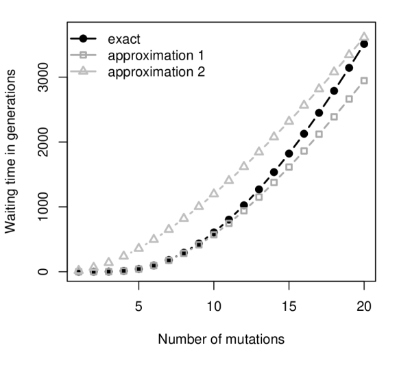
Figure 3: Approximate solutions of the waiting time $\tau_{k}^{*}$ as defined by the equation $1/N=\operatorname{Pois}(k;\mu d\tau_{k}^{*})$, for $N=10^{9}$, $\mu d=0.001$, and $k=1,\dots,20$. The exact solution in terms of the Lambert $W$ function (filled circles, Eq. (28)) is compared to the approximation given in Eq. (29) (squares) and the less accurate but simpler approximation of Eq. (30) (triangles).

The normal mutation rate due to DNA polymerase errors is on the order of $10^{-10}$ to $10^{-9}$ base pairs (bp) per cell per generation (Kunkel and Bebenek, 2000). For an average human gene size of 27kbp (Venter et al., 2001), the mutation rate per gene should be on the order of $\mu\approx 10^{-6}$ per cell per generation. The waiting time until the first of $10^{9}$ cells has accumulated $k=20$ mutations would be on the order of $10^{6}$ cell generations which, in turn, typically occur at the time-scale of days or weeks. Thus, the waiting time would be on the order of $10^{6}$ days or more, clearly exceeding a human lifetime. Hence a neutral evolutionary process alone cannot account for the genetic progression of cancer.

4.2 Selection and clonal expansion

We now analyze the dynamics of an evolving cell population in which each mutation confers the same selective advantage $s>0$. Because a new mutant with an additional mutation has a growth advantage, it will expand in the tissue and outcompete the other cells. The next mutation is most likely to occur on this growing clone. We therefore use an evolutionary model of carcinogenesis that accounts for mutation and selection (Beerenwinkel et al., 2007a) and trace the number of cells with $j$ mutations, $N_{j}(t)$, in each generation $t=0,1,2,\dots$.

Figure 4: Wright-Fisher process. Illustrated are four generations of a single realization of the Wright-Fisher process with population size $N=6$. In each generation $t+1$, cells are drawn randomly from the previous generation $t$ according to the multinomial distribution given in Eq. (31). Directed edges ($\rightarrow$) indicate the genealogy of this realization. In general, cells with more mutations are more likely to generate offspring and will therefore, on average, outcompete cells with fewer mutations. In each generation, cells are subject to mutation ($\rightsquigarrow$). In this realization, the waiting time to the first appearance of a cell with $k=2$ mutations was $\tau_{2}=3$ generations.

Consider a population of $N$ cells that undergo subsequent rounds of cell divisions as shown in Figure 4. In each generation, mutations occur randomly and independently at rate $\mu$. The total number of possible mutations is denoted $d$. We assume that fitness, i.e., the expected number of offspring, is proportional to $(1+s)^{j}$, where $j$ is the number of accumulated mutations. The population dynamics are assumed to follow a Wright-Fisher process (Ewens, 2004). In this model, generations are time-discrete and synchronized. A new configuration $[N_{0}(t+1),\ldots,N_{d}(t+1)]$ of cells is drawn from the previous generation $t$ according to the multinomial distribution

$$\begin{split}\operatorname{Prob}\left[N_{0}(t+1)=n_{0},\dots,N_{d}(t+1)=n_{d}\right]\\ =\frac{(n_{0}+\dots+n_{d})!}{n_{0}!\cdots n_{d}!}\prod_{i=1}^{d}\theta^{n_{j}}_{j},\end{split}$$ (31)

where $n_{0}+\dots+n_{k}=N$. The parameters $\theta_{j}$ denote the probability of sampling a $j$-cell,

$$\theta_{j}=\sum_{i=0}^{j}\binom{d-i}{j-i}\mu^{j-i}(1-\mu)^{d-j}\frac{(1+s)^{i}x_{i}}{\sum_{l}(1+s)^{l}x_{l}},$$ (32)

where we defined $x_{j}(t)=N_{j}(t)/N$ as the relative abundance of $j$-cells. A cell with $j$ mutations can occur in generation $t+1$ either as progeny of a $j$-cell in generation $t$, or by erroneous duplication of a $(j-1)$-cell. For $s=0$ and infinitesimal generation times, the model reduces to the case of independent cell lineages undergoing independent mutations, which has been discussed in the previous section.

In general, no closed form solution of the Wright-Fisher process is known. However, the dynamics defined by Eqs. (31) and (32) display certain regularities that can be exploited in order to derive an approximate analytical expression for the expected waiting time to the first cell with $k$ mutations, $\tau_{k}^{*}$. Numerical simulations show that the subsets of $j$-cells sequentially sweep through the population and the mutant waves travel at constant speed (Beerenwinkel et al., 2007a). This regular behavior can be analyzed by decomposing the process into the generation of a new cell type by mutation and its clonal expansion driven by selection.

The dynamics of clonal expansions are given by the replicator equation (Nowak, 2006),

$$\dot{x}_{j}(t)=sx_{j}(t)\left[j-\sum_{i=1}^{\infty}i\,x_{i}(t)\right],$$ (33)

where we consider only those cell types that are already present in the system and we ignore mutation. The fitness of $j$-cells is $(1+s)^{j}\approx 1+js$, if $s\ll 1$. Eq. (33) has a solution in terms of the Gaussians $x_{j}(t)=A\exp(-[j-vt]^{2}/[2\sigma^{2}])$ with normalization constant $A$ and width $\sigma^{2}=v/s$, where $v$ is the velocity of the traveling wave. The initial growth of a newly founded clone is exponential, but eventually follows this Gaussian distribution. The final decline corresponds to the clone ultimately becoming extinct by outcompetition of fitter clones harboring additional mutations.

The velocity of the waves is determined by the mutation process. A new $(j+1)$-cell is generated by mutation from the growing clone of $j$-cells. The equation $x_{j+1}(t)=1/N$ can therefore be rewritten, similar to Eq. (27), as

$$\int_{0}^{\tau_{j+1}^{*}}\mu dx_{j}(t)\,\mathrm{d}t=\frac{1}{N},$$ (34)

where initially, $x_{j}$ grows exponentially according to Eq. (33). This approach finally yields the approximate expected waiting time (Beerenwinkel et al., 2007a)

$$\tau_{k}^{*}\approx\frac{k\log^{2}(s/[\mu d])}{2s\log N}.$$ (35)

This expression suggests approximating the Wright Fisher process, Eqs. (31) and (32), by a linear multistep process, Eq. (1), with transition rate $u=(2s\log N)/\log^{2}(s/[\mu d])$ in which stages correspond to clonal expansions (Maley, 2007). Comparing Eq. (35) with the waiting time in a neutral evolutionary process, Eq. (30), here the waiting time per mutation, $1/du$, contributes only logarithmically and the expected waiting time Eq. (35) is proportional to $k/s$, reducing the overall waiting time considerably. The reason for this acceleration lies in the growth advantage of the mutated cells: A single cell produces an exponentially growing number of clonal offspring. This growth, in turn, directly relates to the probability of creating a cell with an additional mutation. Therefore, clonal expansions dramatically speed up the accumulation of mutations in a population.

For example, considering a fitness advantage of $s=10^{-2}$ per mutation, $d=100$ susceptible loci, a mutation rate of $u=10^{-7}$ per gene, and a population size of $N=10^{9}$ cells results in a waiting time of $\tau_{20}^{*}\approx 10^{3}$ generations. With a generation time of 1 to 2 days, this waiting time ranges on the time scale of several years, being consistent with clinical observations. By contrast, the waiting time in the neutral model is on the order of $10^{6}$ generations. Hence even a moderate selective advantage decreases the waiting time by three orders of magnitude.

The time $\tau^{*}_{j}$ denotes the time after which the probability that a cell with $j$ mutations has been generated exceeds $1/N$. This is an approximation for the expected waiting time of the first $j$-cell with an additional mutation in a population of size $N$. For the Wright-Fisher process it is known, however, that due to genetic drift the probability of fixation of a selectively advantageous mutation initially present in a single cell is only $2s$ (Ewens, 2004). Hence, the majority of mutated cells become extinct. This is also observed in the numerical simulations of the Wright-Fisher process (Eqs. (31, 32); Beerenwinkel et al. (2007a)). On average it takes $1/2s$ cells until the first successful mutant is generated. This effect is included indirectly in approximation Eq. (35): $x_{j}(t)\propto e^{st}$ is the expected frequency conditioned only on $x_{j}(0)=1/N$ and not on survival. It also accounts for all trajectories, including those going extinct. Recently, this effect has been studied in a related model (Desai and Fisher, 2007; Brunet et al., 2008). Desai and Fisher (2007) found an approximate waiting time of $\tau_{k}^{*}\approx k\log(s/[ud])/(s[2\log N+\log\{sud\}])$. Comparing with expression Eq. (35), the only difference is the term $\log(sud)$ in the denominator. For typical parameter values, $\log(sud)\approx-7\approx-\log N$. Therefore, the waiting time is larger by a factor of $1.5$ as compared to Eq. (35). But this comparison is limited, because the models are not identical. For example, Desai and Fisher (2007) obtain a fixation probability of $s$, whereas in the Wright-Fisher model it is $2s$.

V Conclusion

A quantitative understanding of cancer progression is required for constructing clinical markers and for revealing rate-limiting steps of this process. Here, we have analyzed waiting time models for carcinogenesis and solved the equations defining the expected waiting times. Similar quantities have previously been shown to measure the degree of tumor progression and to predict survival in cancer patients (Rahnenführer et al., 2005).

In the simplest case, carcinogenesis may be described by a linear multistep process. The progression stages are generally described by histological alterations and functional changes, or on a molecular level, by mutation of certain genes and subsequent clonal expansion. In a general multistep process, the overall waiting time to reach stage $k$ is the sum of the waiting times of all predecessing steps.

If tumor stages are defined by the number of mutations that have fixated in the cell population, then the progression dynamics depends on the order in which mutations accumulate. For example, mutations may accumulate in a linear fashion, according to a partial order, or completely independently. Linear accumulation is the slowest and independent progression is the fastest. The acceleration can be considerable, especially if many mutations are available that drive carcinogenesis.

The linear and the independent model present opposing limits of the conjunctive Bayesian network family of models, in which the mutations obey a partial order. The relations of the poset may result from causal relationships among mutations, such as the requirement in colon cancer for the tumor suppressor APC to be mutated before other mutations are beneficial and can fixate. The poset constraints induce a subset of mutational pathways in the hypercube representing all combinatorial genotypes (Figure 2). Because the waiting time is additive in the mutational pathways, its expected value for the conjunctive Bayesian networks ranges between those for the linear and the independent model.

We have discussed a particular instance of the Wright-Fisher process, an evolutionary model comprising mutation and selection. In this model, we find waiting times on the order of 20 years for a normal mutation rate and a selective advantage of 1% per mutation. The successive clonal waves might be regarded as the stages in classical multistage theory. A neutral evolutionary process can not explain the clinical progression of colon cancer, in which about 20 out of hundreds of mutations accumulate in a time frame of 5 to 20 years. This process may only be explained by advantageous mutations giving rise to clonal expansions. These selective sweeps drastically increase the chances of acquiring additional mutations the spreading offspring.

References

- Anderson and Quaranta (2008) Anderson ARA, Quaranta V (2008) Integrative mathematical oncology. Nat Rev Cancer 8:227–234
- Armitage and Doll (1954) Armitage P, Doll R (1954) The age distribution of cancer and a multi-stage theory of carcinogenesis. Br J Cancer 8:1–12
- Baudis (2007) Baudis M (2007) Genomic imbalances in 5918 malignant epithelial tumors: an explorative meta-analysis of chromosomal CGH data. BMC Cancer 7:226
- Beerenwinkel and Sullivant (2008) Beerenwinkel N, Sullivant S (2008) Markov models for accumulating mutations. ArXiv:0709.2646
- Beerenwinkel et al. (2006) Beerenwinkel N, Eriksson N, Sturmfels B (2006) Evolution on distributive lattices. J Theor Biol 242:409–420
- Beerenwinkel et al. (2007a) Beerenwinkel N, Antal T, Dingli D, Traulsen A, Kinzler KW, et al. (2007a) Genetic Progression and the Waiting Time to Cancer. PLoS Comput Biol 3:e225
- Beerenwinkel et al. (2007b) Beerenwinkel N, Eriksson N, Sturmfels B (2007b) Conjunctive Bayesian networks. Bernoulli 13:893–909
- Brunet et al. (2008) Brunet E, Rouzine IM, Wilke CO (2008) The stochastic edge in adaptive evolution. Genetics 179:603–620
- Cairns (1975) Cairns J (1975) Mutation selection and the natural history of cancer. Nature 255:197–200
- Corless et al. (1996) Corless RM, Gonnet GH, Hare DEG, Jeffrey DJ, Knuth DE (1996) On the Lambert W function. Adv Comput Math 5:329–359
- Crespi and Summers (2005) Crespi B, Summers K (2005) Evolutionary biology of cancer. Trends Ecol Evol 20:545–552
- Desai and Fisher (2007) Desai MM, Fisher DS (2007) Beneficial mutation selection balance and the effect of linkage on positive selection. Genetics 176:1759–1798
- Desper et al. (1999) Desper R, Jiang F, Kallioniemi OP, Moch H, Papadimitriou CH, et al. (1999) Inferring tree models for oncogenesis from comparative genome hybridization data. J Comput Biol 6:37–51
- Durrett et al. (2008) Durrett R, Schmidt D, Schweinsberg J (2008) A waiting time problem arising from the study of multi-stage carcinogenesis. ArXiv:0707.2057
- Ewens (2004) Ewens WJ (2004) Mathematical Population Genetics. Springer
- Frank (2007) Frank SA (2007) Dynamics of Cancer: Incidence, Inheritance, and Evolution. Princeton University Press
- Futreal et al. (2004) Futreal PA, Coin L, Marshall M, Down T, Hubbard T, et al. (2004) A census of human cancer genes. Nat Rev Cancer 4:177–183
- Hanahan and Weinberg (2000) Hanahan D, Weinberg RA (2000) The hallmarks of cancer. Cell 100:57–70
- Hjelm et al. (2006) Hjelm M, H glund M, Lagergren J (2006) New probabilistic network models and algorithms for oncogenesis. J Comput Biol 13:853–865
- Humphries and Wright (2008) Humphries A, Wright NA (2008) Colonic crypt organization and tumorigenesis. Nat Rev Cancer 8:415–424
- Iwasa et al. (2005) Iwasa Y, Michor F, Komarova NL, Nowak MA (2005) Population genetics of tumor suppressor genes. J Theor Biol 233:15–23
- Jones et al. (2008a) Jones S, Chen WD, Parmigiani G, Diehl F, Beerenwinkel N, et al. (2008a) Comparative lesion sequencing provides insights into tumor evolution. Proc Natl Acad Sci U S A 105:4283–4288
- Jones et al. (2008b) Jones S, Zhang X, Parsons DW, Lin JCH, Leary RJ, et al. (2008b) Core signaling pathways in human pancreatic cancers revealed by global genomic analyses. Science 321:1801–1806
- Knudson (1971) Knudson AG (1971) Mutation and cancer: statistical study of retinoblastoma. Proc Natl Acad Sci U S A 68:820–823
- Kunkel and Bebenek (2000) Kunkel TA, Bebenek K (2000) DNA replication fidelity. Annu Rev Biochem 69:497–529
- Land et al. (1983) Land H, Parada LF, Weinberg RA (1983) Cellular oncogenes and multistep carcinogenesis. Science 222:771–778
- Ley et al. (2008) Ley TJ, Mardis ER, Ding L, Fulton B, McLellan MD, et al. (2008) DNA sequencing of a cytogenetically normal acute myeloid leukaemia genome. Nature 456:66–72
- Maley (2007) Maley CC (2007) Multistage carcinogenesis in Barrett’s esophagus. Cancer Lett 245:22–32
- Merlo et al. (2006) Merlo LMF, Pepper JW, Reid BJ, Maley CC (2006) Cancer as an evolutionary and ecological process. Nat Rev Cancer 6:924–935
- Michor et al. (2004) Michor F, Iwasa Y, Nowak MA (2004) Dynamics of cancer progression. Nat Rev Cancer 4:197–205
- Mitelman et al. (2008) Mitelman F, Johansson B, Mertens F (2008) Mitelman Database of Chromosome Aberrations in Cancer
- Moolgavkar and Luebeck (1992) Moolgavkar SH, Luebeck EG (1992) Multistage carcinogenesis: population-based model for colon cancer. J Natl Cancer Inst 84:610–618
- Nordling (1953) Nordling CO (1953) A new theory on cancer-inducing mechanism. Br J Cancer 7:68–72
- Nowak (2006) Nowak MA (2006) Evolutionary Dynamics. The Belknap Press of Harvard University Press
- Nowak et al. (2003) Nowak MA, Michor F, Iwasa Y (2003) The linear process of somatic evolution. Proc Natl Acad Sci U S A 100:14966–14969
- Nowak et al. (2006) Nowak MA, Michor F, Iwasa Y (2006) Genetic instability and clonal expansion. J Theor Biol 241:26–32
- Nowell (1976) Nowell PC (1976) The clonal evolution of tumor cell populations. Science 194:23–28
- Parsons et al. (2008) Parsons DW, Jones S, Zhang X, Lin JCH, Leary RJ, et al. (2008) An integrated genomic analysis of human glioblastoma multiforme. Science 321:1807–1812
- Radmacher et al. (2001) Radmacher MD, Simon R, Desper R, Taetle R, Schäffer AA, et al. (2001) Graph models of oncogenesis with an application to melanoma. J Theor Biol 212:535–548
- Rahnenführer et al. (2005) Rahnenführer J, Beerenwinkel N, Schulz WA, Hartmann C, von Deimling A, et al. (2005) Estimating cancer survival and clinical outcome based on genetic tumor progression scores. Bioinformatics 21:2438–2446
- Schinazi (2006) Schinazi RB (2006) A stochastic model for cancer risk. Genetics 174:545–547
- Sidransky (2002) Sidransky D (2002) Emerging molecular markers of cancer. Nat Rev Cancer 2:210–219
- Sjöblom et al. (2006) Sjöblom T, Jones S, Wood LD, Parsons DW, Lin J, et al. (2006) The consensus coding sequences of human breast and colorectal cancers. Science 314:268–274
- Venter et al. (2001) Venter JC, Adams MD, Myers EW, Li PW, Mural RJ, et al. (2001) The sequence of the human genome. Science 291:1304–1351
- Vogelstein and Kinzler (2004) Vogelstein B, Kinzler KW (2004) Cancer genes and the pathways they control. Nat Med 10:789–799
- Wodarz and Komarova (2005) Wodarz D, Komarova NL (2005) Computational Biology of Cancer: Lecture Notes and Mathematical Modeling. World Scientific
- Wood et al. (2007) Wood LD, Parsons DW, Jones S, Lin J, Sjöblom T, et al. (2007) The genomic landscapes of human breast and colorectal cancers. Science 318:1108–1113