Pair correlations of scattered atoms from two colliding Bose-Einstein Condensates: Perturbative Approach.

Abstract

We apply an analytical model for anisotropic, colliding Bose-Einstein condensates in a spontaneous four wave mixing geometry to evaluate the second order correlation function of the field of scattered atoms. Our approach uses quantized scattering modes and the equivalent of a classical, undepleted pump approximation. Results to lowest order in perturbation theory are compared with a recent experiment and with other theoretical approaches.

I Introduction

The analog of correlated photon pair production Burnham and Weinberg (1970) has recently been demonstrated using atoms. Both molecular dissociation Greiner et al. (2005) and four wave mixing of deBroglie waves Perrin et al. (2007) have shown correlation peaks. As in quantum optics, such atom pairs lend themselves to investigations into non-classical correlation phenomena such as entanglement of massive particles Duan et al. (2000); Pu and Meystre (2000); Opatrný and Kurizki (2001); Kheruntsyan et al. (2005) and spontaneous directionality or superradiant effects Pu and Meystre (2000); Vardi and Moore (2002). From the point of view of the outgoing atoms, the underlying physics is very similar and thus theoretical descriptions should be applicable to both processes. The experiment using four wave mixing of metastable helium atoms in particular has yielded detailed information about the atomic pair correlations. Efforts to treat the experimental situations are therefore highly desirable.

Theoretically, the description of condensate collisions in the spontaneous scattering regime requires a formulation that extends beyond the mean-field model Bach et al. (2002); Yurovsky (2002). In previous work on spherical Gaussian wave packets, within perturbative approach, we have given analytical formulas for the correlation functions Ziń et al. (2005, 2006).

In this paper we extend our method to anisotropic condensates to give an analytic description of the correlation properties of spontaneously emitted atom pairs in a geometry much closer to and in good agreement with the experiment Perrin et al. (2007). Numerical approaches using truncated Wigner method Norrie et al. (2005, 2006) and positive-P method Savage et al. (2006); Deuar and Drummond (2007); Perrin et al. (2008) have also been used, in particular to give insight into the stimulation regime where bosonic enhancement comes to play.

Here, we use the model of colliding condensates to examine two types of correlations. First we shall focus on atom pairs originating from the same two body scattering event. These consequently have nearly opposite momenta. Thus we analyze the opposite-momenta correlations of atom pairs. Second, we examine two body correlations between atoms scattered with nearly collinear momenta, a manifestation of the Hanbury Brown-Twiss (HBT) effect Ziń et al. (2005); Savage et al. (2006); Deuar and Drummond (2007); Mølmer et al. (2008). In both cases, the demonstration of a two particle correlation requires a measurement of the conditional probability of detecting a particle at position ${\bf r}_{1}$ given that a particle was detected at ${\bf r}_{2}$. This probability is proportional to the second order correlation function $G^{(2)}({\bf r}_{1},{\bf r}_{2})$ of the field $\hat{\delta}$ of atoms, i.e.

$$G^{(2)}({\bf r}_{1},{\bf r}_{2})={\langle\hat{\delta}^{\dagger}({\bf r}_{1})\hat{\delta}^{\dagger}({\bf r}_{2})\hat{\delta}({\bf r}_{2})\hat{\delta}({\bf r}_{1})\rangle}.$$

We shall pay particular attention to correlations in momentum space and compare these results with experimental data of Perrin et al. (2007). A careful comparison of a numerical treatment based on the positive-P method Perrin et al. (2008) with the experiment Perrin et al. (2007) indicated reasonable agreement, but one of the limitations of the method, the short collision duration which could be simulated, left some unresolved questions. In particular, energy conservation is a less stringent constraint for short collision times, and thus one can wonder about the role this constraint plays in the experiment. The treatment given here is not subject to this limitation and also agrees fairly well with the experiment for most of the experimentally accessible observables. One observable quantity however, the averaged width of the collinear correlation function in a direction orthogonal to the symmetry axis, disagrees with the experiment and with Ref. Perrin et al. (2008). In our treatment, it is precisely the requirement of energy conservation that is at the origin of the difference. At the end of the paper we shall discuss possible explanations of this discrepancy.

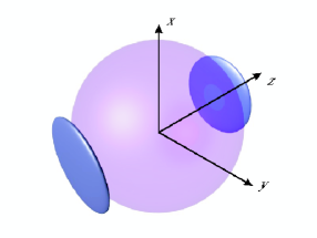
Figure 1: Velocity space representation of the pair production experiment. Raman pulses generate counter-propagating condensates which collide and expand into disk-shaped clouds along the $z$-axis. Atoms scattered during the collision expand to form a spherical shell of correlated pairs. Note that the orientation of the axes in this article differs from Ref. Perrin et al. (2007)

Let us first describe the experiment in which a collision of two Bose-Einstein condensates of metastable helium produces a cloud of scattered atoms. A condensate of approximately 10⁵ He^∗ atoms is created in a cigar-shaped magnetic trap with axial and radial trapping frequencies of $\omega_{z}=2\pi\times$ 47 Hz and $\omega_{r}=2\pi\times$ 1150 Hz respectively. Three laser beams are used to transfer the atoms into two counter-propagating wave-packets by a Raman process, with a transfer efficiency of about 60%. As the wave-packets counter-propagate with a relative velocity of $2v_{rec}=18.4$ cm/s, atoms from the two clouds collide via $s$-wave scattering, populating a spherical shell in momentum space often referred to as the “halo”  Chikkatur et al. (2000); Gibble et al. (1995); Katz et al. (2005). In the experiment, about 5% of the atoms are scattered. In addition to splitting the condensate, the Raman transition transfers the atoms into an untrapped magnetic sub-state. The transferred atoms thus expand freely, falling onto a micro-channel plate (MCP) detector that allows the three-dimensional reconstruction of the position of single atoms with an estimated efficiency of 10% Schellekens et al. (2005); Jeltes et al. (2007). Knowing the positions of individual atoms, the initial momenta, and the second order momentum correlation function of the cloud of scattered particles can be computed. The precision of the measurement is limited by the finite resolution of the MCP. This factor will be taken into account in our comparison between the theoretical estimates and the experimental results.

II Model for scattering

To make the comparison, we introduce a simplified model for atom scattering during a collision of two Bose-Einstein condensate wave-packets. In this model we assume that two counter-propagating wave-packets constitute a classical undepleted source for the process of scattering. This concept is introduced in analogy to examples in quantum optics, where a strong coherent laser field is treated as a classical wave and its depletion is neglected Scully and Zubairy (1997). We shall simplify the model further on. Since we assume that the two colliding condensates remain undepleted, the population of the $\hat{\delta}$ field of scattered atoms should be small, as compared to the number of atoms in the condensates. In such a regime, a Bogoliubov approximation is often used Lifshitz and Pitaevskii (1980); Öhberg et al. (1997), leading to linearized equations of motion for the quantum fields. In our case, the $\hat{\delta}$ field of scattered atoms satisfies the Heisenberg equation (for details of the derivation, see Ziń et al. (2005, 2006))

$$i\hbar\partial_{t}\hat{\delta}({\bf r},t)=-\frac{\hbar^{2}\nabla^{2}}{2m}\hat{\delta}({\bf r},t)+2g\psi_{Q}({\bf r},t)\psi_{-Q}({\bf r},t)\hat{\delta}^{\dagger}({\bf r},t).$$ (1)

Here $\psi_{\pm Q}({\bf r},t)$ is the c-number wave-function of the colliding condensates with mean momentum per atom equal to $\pm\hbar Q$. Moreover, the coupling constant $g=\frac{4\pi\hbar^{2}a}{m}$ is related to the atomic mass $m$ and $s$-wave scattering length $a$ of He^∗.

To permit analytic calculations, we model the condensate wave functions $\psi_{\pm Q}(x,y,z,t)$ as Gaussians:

$$\psi_{\pm Q}=\sqrt{\frac{N}{2\pi^{3/2}\sigma_{r}^{2}\sigma_{z}}}\exp\left(\mp iQz-\frac{i\hbar Q^{2}t}{2m}\right)$$

$$\times\exp\left(-\frac{1}{2\sigma_{r}^{2}}(x^{2}+y^{2})-\frac{1}{2\sigma_{z}^{2}}(z\mp\frac{\hbar Qt}{m})^{2}\right),$$ (2)

where $N$ is the total number of particles in both wave-packets. The radial ($\sigma_{r}$) and axial ($\sigma_{z}$) width of the Gaussians are extracted from the initial condensate wave-function $\Psi_{0}$ which is calculated numerically from the Gross-Pitaevski equation using an imaginary time method. In practice we fit $\int dv_{x}\int dv_{y}|\Psi_{0}(\bf{v})|^{2}$ with a Gaussian function $\propto\exp(-v_{z}^{2}/\chi_{z}^{2})$ and then use $\sigma_{z}=\hbar/(m\;\chi_{z})$. We define $\sigma_{r}$ similarly. Here, for simplicity, we neglect the spread of the condensates during the collision. This assumption seems reasonable because most of the atom collisions take place before the two clouds have had time to expand.

It is useful to change variables and rescale the field operator

$$\frac{\hbar Q}{m\sigma_{z}}t\rightarrow t\ \ \ \ \ \ \ {\bf r}/\sigma_{z}\rightarrow{\bf r}\ \ \ \ \ \ \ \frac{1}{\sigma_{z}^{3/2}}\hat{\delta}({\bf r},t)\rightarrow\hat{\delta}({\bf r},t)$$

which simplifies the equation of motion (1), i.e.

$$i\beta\partial_{t}\hat{\delta}({\bf r},t)=-\frac{1}{2}\nabla^{2}\hat{\delta}({\bf r},t)+\alpha e^{-\frac{x^{2}+y^{2}}{\gamma^{2}}-z^{2}}e^{-i\beta t-t^{2}}\hat{\delta}^{\dagger}({\bf r},t),$$ (3)

where $\alpha=\frac{4Na\sigma_{z}}{\sigma_{r}^{2}\sqrt{\pi}}$, $\beta=Q\sigma_{z}$, $\gamma=\frac{\sigma_{r}}{\sigma_{z}}$.

The condensate density in momentum space then reads,

$$|\Psi_{0}({\bf k})|^{2}=\frac{N\beta^{3}}{\sqrt{\pi^{3}}\,\gamma^{2}}\exp\left[-\beta^{2}(k_{z}^{2}+\gamma^{2}k_{r}^{2})\right]$$ (4)

The three parameters $\alpha,\beta$ and $\gamma$ fully determine the dynamics of the field of scattered atoms. For $N=10^{5}$ and $\hbar Q=mv_{\mathrm{rec}}$ we have $\alpha=1053$, $\beta=227$, and $\gamma=0.05$.

We also find $\chi_{z}=0.004\ v_{\mathrm{rec}}$, $\sigma_{z}=39\ \mu$m, $\chi_{r}=0.0870\ v_{\mathrm{rec}}$ and $\sigma_{r}=2\ \mu$m. The parameter $\alpha$ is a measure of the strength of the interactions between particles. As such, it governs the fraction of atoms scattered into the halo. As a consistency check, in Appendix A we give an alternate estimate of $\alpha$ in the experiment using the observed fraction of scattered atoms.

In Section III we derive an analytical expression for the second order correlation function in the perturbative regime. It is still an open question whether, for these parameters, the perturbative approach applies. We tackle this issue after the evaluation of the $G^{(2)}$ function is Section III.3. In Section IV we compare the perturbative results with the experimental data of Perrin et al. (2007).

III Derivation of $G^{(2)}$ in perturbative regime

We shall begin the analytical calculations with a definition of the Fourier transform of the $\hat{\delta}$ operator

$$\hat{\delta}({\bf r},t)=\left(\frac{\beta}{2\pi}\right)^{3/2}\int d{\bf k}\ e^{i\beta{\bf k}{\bf r}-i\beta k^{2}t/2}\hat{\delta}({\bf k},t).$$ (5)

This particular form of Fourier transformation “incorporates” the free evolution of the field. Substitution of Eq.(5) into Eq.(3) gives

$$\partial_{t}\hat{\delta}({\bf k},t)=\mathcal{A}e^{-i\beta t}e^{-t^{2}}\int d{\bf k}^{\prime}e^{\frac{i\beta}{2}(k^{2}+k^{\prime 2})t}$$

$$\exp\left(-\frac{\gamma^{2}\beta^{2}}{4}({\bf k}_{r}+{\bf k}^{\prime}_{r})^{2}-\frac{\beta^{2}}{4}(k_{z}+k^{\prime}_{z})^{2}\right)\hat{\delta}^{\dagger}({\bf k}^{\prime},t),$$

where $\mathcal{A}=-i\frac{\alpha\beta^{2}\gamma^{2}}{8\pi^{3/2}}$, ${\bf k}_{r}=k_{x}{\bf e}_{x}+k_{y}{\bf e}_{y}$, and ${\bf e}_{i}$ is a unit vector in $i$ direction. The above can be integrated formally, giving

$$\hat{\delta}({\bf k},t)=\mathcal{A}\int_{0}^{t}\mbox{d}\tau\,e^{-i\beta\tau}e^{-\tau^{2}}\int d{\bf k}^{\prime}\,e^{\frac{i\beta}{2}(k^{2}+k^{\prime 2})\tau}$$

$$\exp\left(-\frac{\gamma^{2}\beta^{2}}{4}({\bf k}_{r}+{\bf k}^{\prime}_{r})^{2}-\frac{\beta^{2}}{4}(k_{z}+k^{\prime}_{z})^{2}\right)\hat{\delta}^{\dagger}({\bf k}^{\prime},\tau).$$

Since in the Heisenberg picture the scattered field remains in its initial vacuum state and the evolution of the $\hat{\delta}$ field is linear, the second order correlation function $G^{(2)}({\bf k}_{1},{\bf k}_{2})$ decomposes into

$$G^{(2)}({\bf k}_{1},{\bf k}_{2};t)=\langle\hat{\delta}^{\dagger}({\bf k}_{1},t)\hat{\delta}^{\dagger}({\bf k}_{2},t)\hat{\delta}({\bf k}_{2},t)\hat{\delta}({\bf k}_{1},t)\rangle$$

$$=G^{(1)}({\bf k}_{1},{\bf k}_{1};t)\cdot G^{(1)}({\bf k}_{2},{\bf k}_{2};t)+\left|G^{(1)}({\bf k}_{1},{\bf k}_{2};t)\right|^{2}$$

$$+\left|M({\bf k}_{1},{\bf k}_{2};t)\right|^{2}$$ (6)

where $M({\bf k}_{1},{\bf k}_{2};t)=\langle\hat{\delta}({\bf k}_{1},t)\hat{\delta}({\bf k}_{2},t)\rangle$ is the anomalous density and $G^{(1)}({\bf k}_{1},{\bf k}_{2};t)=\langle\hat{\delta}^{\dagger}({\bf k}_{1},t)\hat{\delta}({\bf k}_{2},t)\rangle$ is the first order correlation function. Below we calculate these two functions in the lowest order and for a time $t=\infty$ because all the measurements are made long after the collision has finished. We expand $\hat{\delta}$ in a series of perturbative solutions,

$$\hat{\delta}({\bf k},t=\infty)=\sum_{i=0}^{\infty}\hat{\delta}^{(i)}({\bf k}).$$

where in the lowest order we get

$$\hat{\delta}^{(1)}({\bf k})=\mathcal{A}\int_{0}^{\infty}\mbox{d}\tau\,e^{-i\beta\tau}e^{-\tau^{2}}\int d{\bf k}^{\prime}\,e^{\frac{i\beta}{2}(k^{2}+k^{\prime 2})\tau}$$ (7)

$$\exp\left(-\frac{\gamma^{2}\beta^{2}}{4}({\bf k}_{r}+{\bf k}^{\prime}_{r})^{2}-\frac{\beta^{2}}{4}(k_{z}+k^{\prime}_{z})^{2}\right)\hat{\delta}^{(0)\dagger}({\bf k}^{\prime}).$$

III.1 Anomalous density: ${\bf k}_{1}\simeq-{\bf k}_{2}$ correlations

The anomalous density in the first order is expressed by

$$M({\bf k}_{1},{\bf k}_{2})=\langle\hat{\delta}^{(0)}({\bf k}_{1})\hat{\delta}^{(1)}({\bf k}_{2})\rangle.$$

Using Eq.(7) we get

$$M({\bf k}_{1},{\bf k}_{2})=\mathcal{A}\exp\left(-\frac{\gamma^{2}\beta^{2}}{4}({\bf k}_{1,r}+{\bf k}_{2,r})^{2}\right)$$

$$\times\exp\left(-\frac{\beta^{2}}{4}(k_{1,z}+k_{1,z})^{2}\right)\int_{0}^{\infty}\mbox{d}\tau\,\exp\left(-i\beta\Delta\tau-\tau^{2}\right),$$

where $\Delta=\beta\left(1-\frac{k_{1}^{2}+k_{2}^{2}}{2}\right)$. This gives

$$M({\bf k}_{1},{\bf k}_{2})=-i\frac{\alpha\beta^{2}\gamma^{2}}{16\pi}\exp\left(-\frac{\beta^{2}}{4}(k_{1,z}+k_{2,z})^{2}\right)$$ (8)

$$\exp\left(-\frac{\gamma^{2}\beta^{2}}{4}({\bf k}_{1,r}+{\bf k}_{2,r})^{2}-\frac{\Delta^{2}}{4}\right)\left(1-\mbox{erf}\left(\frac{i\Delta}{2}\right)\right).$$

This expression shows that the anomalous density describes the correlations of atoms with opposite momenta. In other words, it is non-negligible only when ${\bf k}_{1}\simeq-{\bf k}_{2}$. If this condition is not satisfied, the exponential functions drop quickly. Comparing this expression to Eq.(4), we find that the widths of the anomalous density have the same anisotropy and are two times larger than the condensate density. Moreover, this expression shows that this function is also non-negligible only for $\Delta\lesssim 1$. As $\beta$ is large, $\Delta\sim 1$ only when $k_{1}\simeq 1$ and $k_{2}\simeq 1$. This requirement expresses the conservation of energy in the collision of two atoms.

III.2 First order correlation function: ${\bf k}_{1}\simeq{\bf k}_{2}$ correlations

In the lowest order we have

$$G^{(1)}({\bf k}_{1},{\bf k}_{2})=\langle\hat{\delta}^{(1)\dagger}({\bf k}_{1})\hat{\delta}^{(1)}({\bf k}_{2})\rangle.$$

Using Eq.(7) and $\langle\hat{\delta}^{(0)}({\bf k}_{1})\hat{\delta}^{(0)\dagger}({\bf k}_{2})\rangle=\delta^{(3)}({\bf k}_{1}-{\bf k}_{2})$ we get

$$G^{(1)}({\bf k}_{1},{\bf k}_{2})=|\mathcal{A}|^{2}\int_{0}^{\infty}\mbox{d}\tau\int_{0}^{\infty}\mbox{d}\tau^{\prime}\,\exp\left[-\tau^{2}-\tau^{\prime 2}+i\beta(\tau-\tau^{\prime})\right]\int d{\bf k}\,\exp\left[-\frac{\gamma^{2}\beta^{2}}{4}\left(({\bf k}_{1,r}+{\bf k}_{r})^{2}+({\bf k}_{2,r}+{\bf k}_{r})^{2}\right)\right]$$

$$\times\exp\left[-\frac{\beta^{2}}{4}\left((k_{1,z}+k_{z})^{2}+(k_{2,z}+k_{z})^{2}\right)\right]\exp\left[i\frac{\beta}{2}(k^{2}+k_{2}^{2})\tau^{\prime}-i\frac{\beta}{2}(k^{2}+k_{1}^{2})\tau\right].$$

Under the assumptions that the following three conditions are satisfied

$$\beta\gg 1,\ \ \ \ \ \frac{\gamma}{|{\bf u}_{r}|}\ll 1,\ \ \ \ \ \frac{1}{|{\bf u}_{r}|\beta\gamma}\ll 1,$$ (9)

where ${\bf u}=({\bf k}_{1}+{\bf k}_{2})/|{\bf k}_{1}+{\bf k}_{2}|$ and ${\bf u}_{r}=({\bf k}_{1,r}+{\bf k}_{2,r})/|{\bf k}_{1}+{\bf k}_{2}|$ refers to the radial component of ${\bf u}$.

We show in appendix B that the atomic density is given by

$$G^{(1)}({\bf k},{\bf k})=\frac{\alpha^{2}\beta\gamma^{3}}{32\sqrt{2\pi}|{\bf u}_{r}|}\exp\left[-\frac{2\beta^{2}\gamma^{2}(k-1)^{2}}{|{\bf u}_{r}|^{2}}\right],$$ (10)

and the first order correlation function by

$$G^{(1)}({\bf k}_{1},{\bf k}_{2})=\frac{\alpha^{2}\beta\gamma^{3}}{32\sqrt{2\pi}|{\bf u}_{r}|}\exp\left[-\frac{\gamma^{2}\beta^{2}}{8}\Delta{\bf k}_{r}^{2}-\frac{\beta^{2}}{8}\Delta k_{z}^{2}\right]$$

$$\times\exp\left(-\frac{\beta^{2}}{8}({\bf u}\Delta{\bf k})^{2}\right)\left(1-\mbox{erf}\left(\frac{i\beta{\bf u}\Delta{\bf k}}{2\sqrt{2}}\right)\right)$$

$$\times\exp\left(-\frac{2\beta^{2}\gamma^{2}\Delta K^{2}}{{\bf u}_{r}^{2}}\right).$$ (11)

We have introduced $\frac{|{\bf k}_{1}+{\bf k}_{2}|}{2}=1+\Delta K$, $\Delta{\bf k}={\bf k}_{1}-{\bf k}_{2}$ and assumed $|\Delta{\bf k}|$ is small.

The conditions (9) are fulfilled in the experiment of Ref Perrin et al. (2007) because the region $u_{r}\sim 0$ corresponds to the location of the two condensates and has been excluded from the analysis. The density of the scattered particles is peaked around $k=1$ with a width of $\frac{|{\bf u}_{r}|}{\beta\gamma}\ll 1$. We thus expect an anisotropic halo thickness, but the anisotropy is only strong around $u_{r}\sim 0$, a direction which was inaccessible in the experiment of Ref. Perrin et al. (2007)

As in the case of the anomalous density $M$, we can decompose $G^{(1)}({\bf k}_{1},{\bf k}_{2})$ into factors expressing momentum conservation (1st line of Eq. 11) and energy conservation (2nd line of Eq. 11). We find that the widths of the momentum contribution are $\sqrt{2}$ larger than the corresponding ones for $M({\bf k}_{1},{\bf k}_{2})$ Ziń et al. (2006); Mølmer et al. (2008). As discussed in Refs. [15] and [16], the $\sqrt{2}$ is due to the assumption of a Gaussian density profile. The energy contribution happens to be much more constraining than for $M({\bf k}_{1},{\bf k}_{2})$ because of the term ${\bf u}\Delta{\bf k}$. If ${\bf u}\Delta{\bf k}=0$, meaning $k_{1}=k_{2}$, the width of $G^{(1)}({\bf k}_{1},{\bf k}_{2})$ is given by the momentum contribution. But, if ${\bf u}\Delta{\bf k}\neq 0$ and for instance if ${\bf u}$ is parallel to $\Delta{\bf k}$, its width is $\propto 1/\beta$ even in the radial plane, in contradiction with the simple model developed in Ref.Perrin et al. (2007).

III.3 Applicability of perturbation theory

Perturbation theory is valid provided the scattering of atoms is spontaneous. When bosonic enhancement comes in to play, the perturbative approach fails. Here we give a simple estimate for parameters such as the number of scattered atoms and the dimensionless parameter $\beta$ for which the perturbation is small and the above first order results can be used.

A coherence volume can be attributed to each scattered atom. It is a volume in momentum space in which the atom is first-order coherent. In other words, if we choose a scattered atom with momentum ${\bf k}$, the volume set by all the wave-vectors ${\bf k}_{1}$ for which $|G^{(1)}({\bf k},{\bf k}_{1})|$ is not negligible is the coherence volume. If two bosons scatter in such a way that their coherence volumes overlap, their joint detection amplitude is enhanced by an interference effect. In other words, scattering into an already occupied mode is stimulated. The function $G^{(1)}$ permits an estimate of both the number of scattered atoms and their associated coherence volumes. If the number of scattered atoms is small, coherence volumes are unlikely to overlap, and stimulated scattering is negligible. In this situation we expect our perturbative solution to be valid.

The above argument was used in the case of the collision of two spherically symmetric ($\gamma=1$) Gaussian wave-packets Ziń et al. (2006) and, in comparisons with numerical solutions of the equation for the field $\hat{\delta}$ proved to be correct. Here we apply an analogous reasoning for the case $\gamma\neq 1$. A conservative estimate for the maximum number of scattered atoms for which the perturbative approach applies is $N_{\rm crit}=V/V_{c}$, where $V$ is a lower bound on the $k$-space volume into which atoms are scattered, and $V_{c}$ is an upper bound on the coherence volume of an individual atom.

In the comparison with the experiment (section IV) we analyze a $k$-space volume $\Omega$ which excludes angles $\theta$ smaller than $\pi/4$. From Eq.(10) one sees that the density of scattered atoms is peaked around $k=1$ with an rms width of $\sin\theta/\gamma\beta$. In the volume $\Omega$, the minimum rms width of the shell is $(\gamma\beta\sqrt{2})^{-1}$. Taking twice this minimum rms as the thickness of the shell, we find a lower limit on the volume of $V>4\pi/\gamma\beta$.

The analysis of Eq. (11) shows that $V_{c}$ reaches its maximum in $\Omega$ for $\theta\simeq\pi/4$ (or $\theta\simeq 3\pi/4$, but due to symmetry we will focus on one of these values). If we set $\theta=\pi/4+\delta\theta$, $\varphi=\delta\varphi$ and $k_{1}=k_{2}=1$ we find

$$G^{(1)}(\theta,\ \varphi)\propto\exp\left(-\frac{\beta^{2}(\delta\theta)^{2}}{16}-\frac{\beta^{2}\gamma^{2}(\delta\varphi)^{2}}{16}\right).$$

This gives an angular area of coherence approximately equal to 8$\pi/\gamma\beta^{2}$. Now we need to find the coherence width in the radial direction. Setting ${\bf k}_{1}=(1+\delta k/2){\bf k}/k$ and ${\bf k}_{2}=(1-\delta k/2){\bf k}/k$ we get:

$$G^{(1)}(\delta k)\propto\exp\left(-\frac{\beta^{2}\delta k^{2}}{8}\right).$$

The limit on the coherence volume is therefore: $V_{c}<64\pi/3\gamma\beta^{3}$.

Combining the estimates of $V$ and $V_{c}$, we find that critical number of atoms is given by $N_{\mathrm{crit}}=\frac{3\beta^{2}}{16}$. For $\beta=227$ we get $N_{\mathrm{crit}}\approx 10^{4}$. In the experimental realization, the number of atoms detected in $\Omega$ varied from 30 to 300. Assuming 10% detection efficiency this gives a maximum of 3000 scattered atoms. Thus the experiment should be in the perturbative regime. A similar argument is given in Ref. Perrin et al. (2008) leading to a similar value of $N_{{\rm crit}}$.

IV Comparison with experiment

The formulae (8) and (11) cannot be directly compared with experimental data. This is due to an extra step which is made during the measurements: the joint probabilities measured in experiment are averaged over a region of interest $\Omega$ which excludes the unscattered condensates. We approximate $\Omega$ by $\theta\in[\frac{\pi}{4},\frac{3\pi}{4}]$, $\varphi\in[0,2\pi]$ (where ${\bf u}=(\sin\theta\cos\varphi,\sin\theta\sin\varphi,\cos\theta$)).

In case of local momentum correlations, the normalization procedure is done by choosing ${\bf k}_{1}$ and ${\bf k}_{2}$ almost equal: ${\bf k}_{1}-{\bf k}_{2}=\delta{\bf k}$, where $\delta{\bf k}$ is small. So we set ${\bf k}_{1}={\bf k}+\delta{\bf k}/2$ and ${\bf k}_{2}={\bf k}-\delta{\bf k}/2$. The averaging corresponds to calculation of an integral

$$\langle|G^{(1)}(\delta{\bf k})|^{2}\rangle=\int_{\Omega}d{\bf k}\ |G^{(1)}({\bf k}_{1},{\bf k}_{2})|^{2}.$$ (12)

Then, this function is normalized by

$$\int_{\Omega}d{\bf k}\ G^{(1)}({\bf k}_{1},{\bf k}_{1})\cdot G^{(1)}({\bf k}_{2},{\bf k}_{2}).$$ (13)

Let’s denote the resulting normalized function by $\langle|g^{(1)}(\delta{\bf k})|^{2}\rangle$. As the anomalous density vanishes for local correlations, Eq.(6) gives

$$g^{(2)}(\delta{\bf k})=1+\langle|g^{(1)}(\delta{\bf k})|^{2}\rangle.$$

For $\delta{\bf k}=0$ we get $g^{(2)}(0)=2$ Mølmer et al. (2008).

In case of back-to-back momentum correlations, in analogy we have ${\bf k}_{1}$ and ${\bf k}_{2}$ almost opposite: ${\bf k}_{1}+{\bf k}_{2}=\delta{\bf k}$. We set ${\bf k}_{1}={\bf k}+\delta{\bf k}/2$ and ${\bf k}_{2}=-{\bf k}+\delta{\bf k}/2$. Once again, the averaging corresponds to

$$\langle|M(\delta{\bf k})|^{2}\rangle=\int_{\Omega}d{\bf k}\ |M({\bf k}_{1},{\bf k}_{2})|^{2}.$$

After normalization by function (13) we obtain $\langle|m(\delta{\bf k})|^{2}\rangle$. For the opposite momentum correlations, $G^{(1)}$ vanishes, thus

$$g^{(2)}(\delta{\bf k})=1+\langle|m(\delta{\bf k})|^{2}\rangle.$$

Let us now calculate the normalization function from (13), as it is common for both local- and opposite- momentum correlations. From Eq.(11) we have

$$G^{(1)}({\bf k}_{1,2})=\frac{\alpha^{2}\beta\gamma^{3}\sqrt{\pi}}{32\pi\sqrt{2}|{\bf u}_{1,2r}|}\exp\left[-\frac{\beta^{2}\gamma^{2}(k_{1,2}^{2}-1)^{2}}{2|{\bf u}_{1,2r}|^{2}}\right].$$

Now, in spherical coordinates, $|{\bf u}_{1,2r}|=|\sin\theta_{1,2}|$, where $\theta_{1,2}$ is an angle between vector ${\bf k}_{1,2}$ and axis $z$. Since $\frac{1}{2}\delta{\bf k}$ is much smaller than ${\bf k}$, we can approximate $\sin\theta_{1,2}\simeq\sin\theta$, where $\theta$ is an angle between vector ${\bf k}$ and axis $z$ and drop higher order terms in $\delta{\bf k}$ in the exponentials. We end up with the approximate expression

$$\int_{\Omega}d{\bf k}\ G^{(1)}({\bf k}_{1},{\bf k}_{1})\cdot G^{(1)}({\bf k}_{2},{\bf k}_{2})\simeq\frac{\alpha^{4}\beta^{2}\gamma^{6}}{2^{11}\pi\sin^{2}\theta}$$

$$\times\int_{\Omega}d{\bf k}\ \exp\left[-\frac{\beta^{2}\gamma^{2}(k^{2}-1)^{2}}{\sin^{2}\theta}-\frac{\beta^{2}\gamma^{2}({\bf k}\cdot\delta{\bf k})^{2}}{\sin^{2}\theta}\right].$$

If $\delta{\bf k}=\delta k\cdot{\bf e}_{x}$, ${\bf k}\cdot\delta{\bf k}=k\delta k\sin\theta\cos\phi$ and if $\delta{\bf k}=\delta k\cdot{\bf e}_{z}$, ${\bf k}\cdot\delta{\bf k}=k\delta k\cos\theta$. The resulting integrals are calculated numerically.

IV.1 Back to back momentum correlations

As discussed above, we set ${\bf k}_{1}={\bf k}+\delta{\bf k}/2$ and ${\bf k}_{2}=-{\bf k}+\delta{\bf k}/2$. Using Eq.(8)

$$|M({\bf k}_{1},{\bf k}_{2})|^{2}=\frac{\alpha^{2}\beta^{4}\gamma^{4}}{256\pi^{2}}\exp\left(-\frac{\gamma^{2}\beta^{2}}{2}\delta k_{r}^{2}-\frac{\beta^{2}}{2}\delta k_{z}^{2}-\frac{\Delta^{2}}{4}\right)$$

$$\left(1+\mbox{erfi}^{2}\left(\frac{\Delta}{2}\right)\right).$$

Here, $\Delta=\beta(1-k^{2}-\frac{\delta k^{2}}{4})$. The averaging over $\Omega$ is equivalent to

$$\langle|M(\delta{\bf k})|^{2}\rangle=\int_{\Omega}d{\bf k}\ |M({\bf k}_{1},{\bf k}_{2})|^{2}=\frac{\alpha^{2}\beta^{4}\gamma^{4}}{256\pi^{2}}e^{-\frac{\gamma^{2}\beta^{2}}{2}\delta k_{r}^{2}}$$

$$\times e^{-\frac{\beta^{2}}{2}\delta k_{z}^{2}}\int_{\Omega}d{\bf k}\ e^{-\frac{\Delta^{2}}{4}}\left(1+\mbox{erfi}^{2}\left(\frac{\Delta}{2}\right)\right).$$

Numerical evaluation of this integral (for parameters $\beta$ and $\gamma$ as defined above) shows that the averaged anomalous density can be well-approximated by

$$\langle|M(\delta{\bf k})|^{2}\rangle\propto\exp\left(-\frac{\gamma^{2}\beta^{2}}{2}\delta k_{r}^{2}-\frac{\beta^{2}}{2}\delta k_{z}^{2}\right).$$

As we see, the width of $\langle|M(\delta{\bf k})|^{2}\rangle$ is primarily determined by the momentum conservation constraint, but the analysis shows that energy conservation plays a role, decreasing the predicted width in the $xy$-plane by of order 10%. We normalize the second order correlation function by (13) and introduce an empirical parameter $\eta_{\mathrm{bb}}$ to account for the fact that in the experimental data plots, the correlation functions are projections, and the fact that their heights were smaller than expected. We find

$$g^{(2)}(\delta{\bf k})=1+\eta_{\mathrm{bb}}\langle|m(\delta{\bf k})|^{2}\rangle.$$

This function is plotted in Fig. 2, using the value $\eta_{\mathrm{bb}}=0.032$. We find good agreement with the experimental data in the $x$- and $y$- directions. In the $z$-direction, the width of the experimental peak is dominated by the detector resolution which is larger than the calculated width.

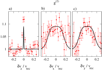
Figure 2: (color online): Normalized opposite momentum correlations calculated in perturbative regime as compared with experimental data. Three plots correspond to three different directions. Here, $\delta v_{i}=\hbar/m\cdot\delta k_{i}$ and $v_{rec}=\hbar/m\cdot Q$.

IV.2 Local momentum correlations

For the collinear correlation function we choose ${\bf k}_{1}={\bf k}+\delta{\bf k}/2$ and ${\bf k}_{2}={\bf k}-\delta{\bf k}/2$. Using Eq.(11) and definition from Eq.(12) we have

$$\langle|G^{(1)}(\delta{\bf k})|^{2}\rangle=\int_{\Omega}d{\bf k}\ \frac{\alpha^{4}\beta^{2}\gamma^{6}}{2^{11}\pi|{\bf u}_{r}|^{2}}\exp\left(-\frac{\beta^{2}}{4}({\bf u}\delta{\bf k})^{2}\right)$$

$$\exp\left[-\frac{\gamma^{2}\beta^{2}}{4}\delta{\bf k}_{r}^{2}-\frac{\beta^{2}}{4}\delta k_{z}^{2}\right]\left[1+\mbox{erfi}^{2}\left(\frac{\beta}{2\sqrt{2}}{\bf u}\delta{\bf k}\right)\right]$$

$$\times\exp\left(-\frac{4\beta^{2}\gamma^{2}(k-1)^{2}}{{\bf u}_{r}^{2}}\right).$$

Let us now consider two separate cases.

Let’s set $\delta{\bf k}=\delta k_{x}{\bf e}_{x}$. Then, ${\bf u}\delta{\bf k}=\delta k\sin\theta\cos\varphi$. Integration over the region $\Omega$ consists of an angular and a radial integral. The radial one is

$$I_{r}=\int_{0}^{\infty}k^{2}dk\times\exp\left(-\frac{4\beta^{2}\gamma^{2}(k-1)^{2}}{{\bf u}_{r}^{2}}\right).$$

The width of this Gaussian function is so small, that we can set $k^{2}dk\sim dk$. Setting $k=1+dk$ and extending the lower limit of the integral to $-\infty$ gives $I_{r}\propto|{\bf u}_{r}|$. Thus

$$\langle|G^{(1)}(\delta k_{x})|^{2}\rangle\propto e^{-\frac{\gamma^{2}\beta^{2}}{4}\delta k_{x}^{2}}\int_{0}^{2\pi}d\varphi\int_{\pi/4}^{3/4\pi}d\theta$$

$$\exp\left(-\frac{\beta^{2}}{4}\delta k_{x}^{2}\cdot u^{2}(\theta,\varphi)\right)\left[1+\mbox{erfi}^{2}\left(\frac{\beta\cdot\delta k_{x}}{2\sqrt{2}}u(\theta,\varphi)\right)\right],$$

where $u(\theta,\varphi)=\sin\theta\cos\varphi$. This integral is calculated numerically and we obtain

$$\langle g^{(2)}(\delta k_{x})\rangle=1+\langle|g^{(1)}(\delta k_{x})|^{2}\rangle.$$

The result is again rescaled by the parameter $\eta_{\mathrm{c}l}$ although it needs not to be identical to the back to back case:

$$\langle g^{(2)}(\delta k_{x})\rangle=1+\eta_{\mathrm{c}l}\langle|g^{(1)}(\delta k_{x})|^{2}\rangle.$$

As $\langle|g^{(1)}(0)|^{2}\rangle=1$, we deduce the value of $\eta_{\mathrm{cl}}=0.05$.

Now we set $\delta{\bf k}=\delta k_{z}{\bf e}_{z}$, and therefore ${\bf u}\delta{\bf k}=\delta k_{z}\cos\theta$. The radial integral is the same as in the previous case and we find

$$\langle|G^{(1)}(\delta k_{z})|^{2}\rangle\propto\exp\left[-\frac{\beta^{2}}{4}(\delta k_{z})^{2}\right]\int_{\pi/4}^{3/4\pi}d\theta$$

$$\exp\left(-\frac{\beta^{2}}{4}(\delta k_{z})^{2}\cdot\cos^{2}\theta\right)\left[1+\mbox{erfi}^{2}\left(\frac{\beta\cdot\delta k_{z}}{2\sqrt{2}}\cos\theta\right)\right].$$

Numerically we find:

$$\langle g^{(2)}(\delta k_{z})\rangle=1+\eta_{\mathrm{cl}}\langle|g^{(1)}(\delta k_{z})|^{2}\rangle.$$

We find that chosing $\eta_{\mathrm{cl}}=0.05$ makes the observed heights match.

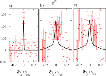
Figure 3: (color online): Normalized collinear correlations calculated in perturbative regime as compared with experimental data. Three plots correspond to three different directions. Due to cylindrical symmetry of the colliding condensates, theoretical results preserve this symmetry. Here, $\delta v_{i}=\hbar/m\cdot\delta k_{i}$ and $v_{rec}=\hbar/m\cdot Q$.

Once again, because of the detector resolution, we find that the calculated peak is much narrower that the observed one in the $z$-direction. What is more surprising is that the widths of the correlation functions in the $x$- and $y$-directions are also narrower than those in the experiment. As can be seen from the discussion following Eq.(11), the peak width along the direction of the outgoing atoms is strongly constrained by the energy conservation requirement. This means that for scattering far from the $z$-axis ($\theta$ large), the $x$- and $y$-components of the correlation function are narrower than they would be taking momentum conservation alone into account. This result contradicts the simple reasoning of Ref. Perrin et al. (2007). In the next section we speculate about why neither the experiment nor the positive P simulation results reproduce the above width for the correlation function.

V Conclusions

The perturbative result we have presented here, while rather complex, has the virtue that the results are analytic and permit the identification the physical processes involved in the pair formation process. In particular the roles of energy and momentum conservation are clearly identified. Our results for the back to back correlation are in good agreement with the experiment. On the other hand the collinear correlation function, as shown in Fig. 3, is in apparent contradiction with both the experiment and with the calculation of Ref. Perrin et al. (2008). The perturbative correlation function given in this work is narrower. This discrepancy clearly needs more attention, both theoretical and experimental, but we wish to make some comments about possible causes. First, as discussed in Ref. Perrin et al. (2008), the calculations using the positive P representation are not able to simulate the entire duration of the collision; indeed only about 20% of the collision time can be simulated. Thus, energy conservation is not as strictly enforced leading to additional broadening in the calculations of Ref. Perrin et al. (2008). Although this effect was discussed in that reference, the problem requires further scrutiny, it is not entirely clear to us which widths are most affected by a short collision time. Second, the experimental observations are also subject to effects not treated here. It was briefly mentioned in Ref. Perrin et al. (2007) that the mean field interaction between the escaping atoms and the remaining condensates may not be negligible. It is therefore important to undertake an analysis of their effect on the correlation functions. Finally, an important simplification in the present treatment is the assumption that the condensates do not expand during the collision. This assumption seems reasonable because most of the atom collisions take place before the clouds have had time to expand. Still, a quantitative estimate of the influence of the condensate expansion is another avenue for future analysis.

Clarifying these questions may have ramifications beyond atom optics. Conceptually similar experiments involving collisions between heavy ions have also uncovered discrepancies between observations and simple models Lisa et al. (2005); Wong and Zhang (2007), the so-called “HBT puzzle”. We hope that the work presented here will continue to stimulate careful thought about the four wave mixing process of matter waves.

VI Acknowledgements

We acknowledge the support of the CIGMA project of the Eurocores program of ESF, the SCALA project of the EU and the Institut Francilien pour la Recherche en Atomes Froids. P Z. and J. Ch. acknowledge the support of Polish Government scientific grant (2007-2010).

Appendix A Determination of $\alpha$

When we introduced $\alpha$, it was simply defined in terms of the number of atoms, the condensate size and the scattering length. Here we give a complementary estimate of $\alpha$ which provides a consistency check. The result essentially shows that our treatment is able to predict, to within experimental uncertainties, the number of scattered atoms. We start from Eq.(10). The integration of this equation over $\Omega$ gives the number of scattered atoms to first order. This result, being a function of $\alpha$, can be compared with the number of scattered atoms in the experiment. Knowing this number, we can evaluate $\alpha$. First, using Eq.(10), the number of scattered atoms in $\Omega$ is given by

$$\mathcal{N}_{\Omega}=\frac{\alpha^{2}\beta\gamma^{3}}{32\sqrt{2\pi}|{\bf u}_{r}|}\int_{\Omega}d{\bf k}\exp\left[-\frac{\beta^{2}\gamma^{2}(k^{2}-1)^{2}}{2|{\bf u}_{r}|^{2}}\right].$$

Let us focus for a moment on the radial part of the above integral,

$$I_{\mathrm{rad}}=\frac{\alpha^{2}\beta\gamma^{3}}{32\sqrt{2\pi}|{\bf u}_{r}|}\int_{0}^{\infty}k^{2}dk\exp\left[-\frac{\beta^{2}\gamma^{2}(k^{2}-1)^{2}}{2|{\bf u}_{r}|^{2}}\right].$$

First, as the integrand is strongly peaked around $k=1$, the measured volume can be dropped, i.e. $k^{2}\sim 1$. Then, introducing $k=1+\delta k$ and assuming $\delta k$ is small we get

$$I_{\mathrm{rad}}\simeq\frac{\alpha^{2}\beta\gamma^{3}}{32\sqrt{2\pi}|{\bf u}_{r}|}\int_{-1}^{\infty}d(\delta k)\exp\left[-\frac{\beta^{2}\gamma^{2}(\delta k)^{2}}{2|{\bf u}_{r}|^{2}}\right].$$

The lower limit can be extended to $-\infty$, giving

$$I_{\mathrm{rad}}\simeq\frac{\alpha^{2}\beta\gamma^{3}}{32\sqrt{2\pi}|{\bf u}_{r}|}\int_{-\infty}^{\infty}d(\delta k)\exp\left[-\frac{\beta^{2}\gamma^{2}(\delta k)^{2}}{2|{\bf u}_{r}|^{2}}\right]=\frac{\alpha^{2}\gamma^{2}}{64}.$$

Integration over the angular variables gives a factor of $2\sqrt{2}\pi$ and

$$\mathcal{N}_{\Omega}=\frac{\pi\sqrt{2}}{32}\alpha^{2}\gamma^{2}.$$

From the experimental data we know that the number of scattered atoms varies from 300 to 3000. For $N_{\Omega}=300$ we get $\alpha=930$ and for $N_{\Omega}=3000$ we get $\alpha=2940$. Thus the value of $\alpha=1053$ calculated from the model of colliding Gaussians lies somewhere in between. This result, confirms that the choice of parameters such as $\sigma_{r}$ and $\sigma_{z}$ are reasonable.

Appendix B First order correlation function: ${\bf k}_{1}\simeq{\bf k}_{2}$ correlations

To first order the $G^{(1)}$ function is,

$$G^{(1)}({\bf k}_{1},{\bf k}_{2})=|\mathcal{A}|^{2}\int_{0}^{\infty}\mbox{d}\tau\int_{0}^{\infty}\mbox{d}\tau^{\prime}\,\exp\left[-\tau^{2}-\tau^{\prime 2}+i\beta(\tau-\tau^{\prime})\right]\int d{\bf k}\,\exp\left[-\frac{\gamma^{2}\beta^{2}}{4}\left(({\bf k}_{1,r}+{\bf k}_{r})^{2}+({\bf k}_{2,r}+{\bf k}_{r})^{2}\right)\right]$$

$$\times\exp\left[-\frac{\beta^{2}}{4}\left((k_{1,z}+k_{z})^{2}+(k_{2,z}+k_{z})^{2}\right)\right]\exp\left[i\frac{\beta}{2}(k^{2}+k_{2}^{2})\tau^{\prime}-i\frac{\beta}{2}(k^{2}+k_{1}^{2})\tau\right].$$

Thus, in contrast to the anomalous density, we must perform a two-fold time as well as a three-dimensional space integral. The space integral can be evaluated analytically. Then, introducing $x=\frac{\tau+\tau^{\prime}}{\sqrt{2}}$ and $y=\frac{\tau-\tau^{\prime}}{\sqrt{2}}$ the first order correlation function is

$$G^{(1)}({\bf k}_{1},{\bf k}_{2})=\frac{\alpha^{2}\beta\gamma^{2}}{16\pi^{3/2}\sqrt{2}}\exp\left[-\frac{\gamma^{2}\beta^{2}}{8}|{\bf k}_{1,r}-{\bf k}_{2,r}|^{2}-\frac{\beta^{2}}{8}|k_{1,z}-k_{2,z}|^{2}\right]\int_{0}^{\infty}\mbox{d}x\int_{-x}^{x}\mbox{d}y\,\exp\left[-x^{2}+i\frac{\beta}{2\sqrt{2}}x(k_{2}^{2}-k_{1}^{2})\right]$$

$$\times\exp\left[-y^{2}\left(1+\frac{{\bf u}_{r}^{2}}{\gamma^{2}}+{\bf u}_{z}^{2}\right)+i\beta\sqrt{2}y\left(1-\frac{k_{1}^{2}+k_{2}^{2}}{4}-\frac{({\bf k}_{1}+{\bf k}_{2})^{2}}{8}\right)\right]\exp\left[i\sqrt{2}y\frac{({\bf k}_{1,r}+{\bf k}_{2,r})^{2}}{4}\frac{y^{2}}{\gamma^{2}(\beta\gamma^{2})}\frac{1}{1+2y^{2}/(\beta\gamma^{2})^{2}}\right]$$

$$\times\exp\left[\frac{y^{2}}{\gamma^{2}}\left({\bf u}_{r}^{2}-\frac{({\bf k}_{1,r}+{\bf k}_{2,r})^{2}}{4(1+2y^{2}/(\beta\gamma^{2})^{2})}\right)\right]\exp\left[i\sqrt{2}y\frac{(k_{1,z}+k_{2,z})^{2}}{4}\frac{y^{2}}{\beta}\frac{1}{1+2y^{2}/\beta^{2}}\right]\exp\left[y^{2}\left({\bf u}_{z}^{2}-\frac{({\bf k}_{1,r}+{\bf k}_{2,r})^{2}}{4(1+2y^{2}/\beta^{2})}\right)\right]$$

$$\times\frac{1}{1+i\sqrt{2}y/(\beta\gamma^{2})}\frac{1}{\sqrt{1+i\sqrt{2}y/\beta}}$$

where ${\bf u}={\bf u}_{r}+{\bf u}_{z}$ is a vector of unit length and direction ${\bf k}_{1}+{\bf k}_{2}$. As the scattering of atoms conserves energy and momentum, we expect that the density of atoms should be centered around $|{\bf k}|=1$ (which corresponds to $|{\bf k}|=Q$ in physical units). Moreover, from the factor $\exp\left[-y^{2}\left(1+\frac{{\bf u}_{r}^{2}}{\gamma^{2}}+{\bf u}_{z}^{2}\right)\right]$, we deduce that the characteristic width of variable $y$ is $1/\sqrt{1+\frac{{\bf u}_{r}^{2}}{\gamma^{2}}+{\bf u}_{z}^{2}}$.

Using the second of conditions (9) we have

$$\exp\left[-y^{2}\left(1+\frac{{\bf u}_{r}^{2}}{\gamma^{2}}+{\bf u}_{z}^{2}\right)\right]\simeq\exp\left[-y^{2}\frac{{\bf u}_{r}^{2}}{\gamma^{2}}\right].$$

Since the characteristic range of $y$ is $\gamma/|{\bf u}_{r}|$, all the terms proportional to $y/\beta$ and $y/\beta\gamma^{2}$ can be dropped. This gives

$$G^{(1)}({\bf k}_{1},{\bf k}_{2})=\frac{\alpha^{2}\beta\gamma^{2}}{16\pi^{3/2}\sqrt{2}}\exp\left[-\frac{\gamma^{2}\beta^{2}}{8}|{\bf k}_{1,r}-{\bf k}_{2,r}|^{2}-\frac{\beta^{2}}{8}|k_{1,z}-k_{2,z}|^{2}\right]\int_{0}^{\infty}\mbox{d}x\int_{-x}^{x}\mbox{d}y\,\exp\left[-x^{2}+i\frac{\beta}{2\sqrt{2}}x(k_{2}^{2}-k_{1}^{2})\right]$$

$$\times\exp\left[-\frac{y^{2}}{\gamma^{2}}{\bf u}_{r}^{2}+i\beta\sqrt{2}y\left(1-\frac{k_{1}^{2}+k_{2}^{2}}{4}-\frac{({\bf k}_{1}+{\bf k}_{2})^{2}}{8}\right)+\frac{y^{2}}{\gamma^{2}}\left({\bf u}_{r}^{2}-\frac{({\bf k}_{1,r}+{\bf k}_{2,r})^{2}}{4}\right)\right].$$ (14)

Now, by letting ${\bf k}_{1}={\bf k}_{2}={\bf k}$ in Eq.(14) let us focus on the momentum density of scattered atoms,

$$G^{(1)}({\bf k},{\bf k})=\frac{\alpha^{2}\beta\gamma^{2}}{16\pi^{3/2}\sqrt{2}}\int_{0}^{\infty}\mbox{d}x\,\exp\left[-x^{2}\right]$$

$$\int_{-x}^{x}\mbox{d}y\,\exp\left[-\frac{y^{2}}{\gamma^{2}}{\bf u}_{r}^{2}+i\beta\sqrt{2}y\left(1-k^{2}\right)\right]$$

$$\times\exp\left[\frac{y^{2}}{\gamma^{2}}{\bf u}_{r}^{2}(1-k^{2})\right]$$

From the above we deduce that the characteristic width of $x$ is $1$ which is much larger that the characteristic width of $y$. This allows another approximation – the limits of $y$ integral can be expanded up from $-\infty$ to $\infty$. The variables $y$ and $x$ effectively decouple, giving

$$G^{(1)}({\bf k},{\bf k})=\frac{\alpha^{2}\beta\gamma^{2}}{32\pi\sqrt{2}}\int_{-\infty}^{\infty}\exp\left[-\frac{y^{2}}{\gamma^{2}}{\bf u}_{r}^{2}+i\beta\sqrt{2}y\left(1-k^{2}\right)\right]$$

$$\times\exp\left[\frac{y^{2}}{\gamma^{2}}{\bf u}_{r}^{2}(1-k^{2})\right]\mbox{d}y.$$

After integration over $y$ and with $k\sim 1$, one obtains,

$$G^{(1)}({\bf k},{\bf k})=\frac{\alpha^{2}\beta\gamma^{3}}{32\sqrt{2\pi}|{\bf u}_{r}|}\exp\left[-\frac{2\beta^{2}\gamma^{2}(k-1)^{2}}{|{\bf u}_{r}|^{2}}\right].$$

Equation (14) can be rewritten in the form

$$G^{(1)}({\bf k}_{1},{\bf k}_{2})=\frac{\alpha^{2}\beta\gamma^{2}}{16\pi^{3/2}\sqrt{2}}\exp\left[-\frac{\gamma^{2}\beta^{2}}{8}|{\bf k}_{1,r}-{\bf k}_{2,r}|^{2}-\frac{\beta^{2}}{8}|k_{1,z}-k_{2,z}|^{2}\right]\int_{0}^{\infty}\mbox{d}x\int_{-x}^{x}\mbox{d}y\,\exp\left[-x^{2}+i\frac{\beta}{2\sqrt{2}}x(k_{2}^{2}-k_{1}^{2})\right]$$

$$\times\exp\left[-\frac{y^{2}}{\gamma^{2}}{\bf u}_{r}^{2}+i\beta\sqrt{2}y\left(1-\frac{k_{1}^{2}+k_{2}^{2}}{4}-\frac{({\bf k}_{1}+{\bf k}_{2})^{2}}{8}\right)+\frac{y^{2}}{\gamma^{2}}\left({\bf u}_{r}^{2}-\frac{({\bf k}_{1,r}+{\bf k}_{2,r})^{2}}{4}\right)\right].$$

Introducing $\frac{|{\bf k}_{1}+{\bf k}_{2}|}{2}=1+\Delta K$ and $\Delta{\bf k}={\bf k}_{1}-{\bf k}_{2}$, where $|\Delta{\bf k}|$ is small we obtain

$$G^{(1)}({\bf k}_{1},{\bf k}_{2})=\frac{\alpha^{2}\beta\gamma^{3}}{32\sqrt{2\pi}|{\bf u}_{r}|}\exp\left[-\frac{\gamma^{2}\beta^{2}}{8}\Delta{\bf k}_{r}^{2}-\frac{\beta^{2}}{8}\Delta k_{z}^{2}\right]$$

$$\times\exp\left(-\frac{\beta^{2}}{8}({\bf u}\Delta{\bf k})^{2}-\frac{2\beta^{2}\gamma^{2}\Delta K^{2}}{{\bf u}_{r}^{2}}\right)\left(1-\mbox{erf}\left(\frac{i\beta{\bf u}\Delta{\bf k}}{2\sqrt{2}}\right)\right).$$

References

- Burnham and Weinberg (1970) D. C. Burnham and D. L. Weinberg, Phys. Rev. Lett. 25, 84 (1970).
- Greiner et al. (2005) M. Greiner, C. A. Regal, J. T. Stewart, and D. S. Jin, Phys. Rev. Lett. 94, 110401 (2005).
- Perrin et al. (2007) A. Perrin, H. Chang, V. Krachmalnicoff, M. Schellekens, D. Boiron, A. Aspect, and C. I. Westbrook, Phys. Rev. Lett. 99, 150405 (2007),
- Duan et al. (2000) L.-M. Duan, A. Sørensen, J. I. Cirac, and P. Zoller, Phys. Rev. Lett. 85, 3991 (2000).
- Pu and Meystre (2000) H. Pu and P. Meystre, Phys. Rev. Lett. 85, 3987 (2000).
- Opatrný and Kurizki (2001) T. Opatrný and G. Kurizki, Phys. Rev. Lett. 86, 3180 (2001).
- Kheruntsyan et al. (2005) K. V. Kheruntsyan, M. K. Olsen, and P. D. Drummond, Phys. Rev. Lett. 95, 150405 (2005).
- Vardi and Moore (2002) A. Vardi and M. G. Moore, Phys. Rev. Lett. 89, 090403 (2002).
- Bach et al. (2002) R. Bach, M. Trippenbach, and K. Rza¸żewski, Phys. Rev. A 65, 063605 (2002).
- Yurovsky (2002) V. A. Yurovsky, Phys. Rev. A 65, 033605 (2002).
- Ziń et al. (2005) P. Ziń, J. Chwedeńczuk, A. Veitia, K. Rza̧żewski, and M. Trippenbach, Phys. Rev. Lett. 94, 200401 (2005).
- Ziń et al. (2006) P. Ziń, Chwedeńczuk, and M. Trippenbach, Phys. Rev. A 73, 033602 (2006).
- Norrie et al. (2005) A. A. Norrie, R. J. Ballagh, and C. W. Gardiner, Phys. Rev. Lett. 94, 040401 (2005).
- Norrie et al. (2006) A. A. Norrie, R. J. Ballagh, and C. W. Gardiner, Phys. Rev. A 73, 043617 (2006).
- Savage et al. (2006) C. M. Savage, P. E. Schwenn, and K. V. Kheruntsyan, Phys. Rev. A 74, 033620 (2006).
- Deuar and Drummond (2007) P. Deuar and P. D. Drummond, Phys. Rev. Lett. 98, 120402 (2007).
- Perrin et al. (2008) A. Perrin, C. M. Savage, D. Boiron, V. Krachmalnicoff, C. I. Westbrook, and K. V. Kheruntsyan, New J. Phys. 10, 045021 (2008).
- Mølmer et al. (2008) K. Mølmer, A. Perrin, V. Krachmalnicoff, V. Leung, D. Boiron, A. Aspect, and C. I. Westbrook, Phys. Rev. A 77, 033601 (2008),
- Chikkatur et al. (2000) A. Chikkatur, A. Görlitz, D. Stamper-Kurn, S. Inouye, S. Gupta, and W. Ketterle, Phys. Rev. Lett. 85, 483 (2000).
- Gibble et al. (1995) K. Gibble, S. Chang, and R. Legere, Phys. Rev. Lett. 75, 2666 (1995).
- Katz et al. (2005) N. Katz, E. Rowen, R. Ozeri, and N. Davidson, Phys. Rev. Lett. 95, 220403 (2005).
- Schellekens et al. (2005) M. Schellekens, R. Hoppeler, A. Perrin, J. Viana Gomes, D. Boiron, C. I. Westbrook, and A. Aspect, Science 310, 648 (2005).
- Jeltes et al. (2007) T. Jeltes, J. M. McNamara, W. Hogervorst, W. Vassen, V. Krachmalnicoff, M. Schellekens, A. Perrin, H. Chang, D. Boiron, A. Aspect, et al., Nature 445, 402 (2007).
- Scully and Zubairy (1997) M. O. Scully and M. S. Zubairy, Quantum Optics (Cambridge University Press; 1 edition (September 28, 1997), 1997).
- Lifshitz and Pitaevskii (1980) E. M. Lifshitz and L. P. Pitaevskii, Statistical Physics, Part 2 (Pergamon Press, Oxford, 1980).
- Öhberg et al. (1997) P. Öhberg, E. L. Surkov, I. Tittonen, S. Stenholm, M. Wilkens, and G. V. Shlyapnikov, Phys. Rev. A 56, R3346 (1997).
- Lisa et al. (2005) M. Lisa, S. Pratt, R. Stoltz, and U. Wiedemann, Ann. Rev. Nucl. Part.Sci. 55, 357 (2005).
- Wong and Zhang (2007) C.-Y. Wong and W.-N. Zhang, Phys. Rev. C 76, 034905 (2007).