Do metals exist in two dimensions?
A study of many-body localisation in low density electron gases.

Abstract

Using a combination of ground state quantum Monte-Carlo and finite size scaling techniques, we perform a systematic study of the effect of Coulomb interaction on the localisation length of a disordered two-dimensional electron gas. We find that correlations delocalise the 2D system. In the absence of valley degeneracy (as in GaAs heterostructures), this delocalization effect corresponds to a finite increase of the localization length. The delocalisation is much more dramatic in the presence of valley degeneracy (as in Si MOSFETSs) where the localization length increases drastically. Our results suggest that a rather simple mechanism can account for the main features of the metallic behaviour observed in high mobility Si MOSFETs. Our findings support the claim that this behaviour is indeed a genuine effect of the presence of electron-electron interactions, yet that the system is not a “true” metal in the thermodynamic sense.

Since the discovery of Anderson localisation Anderson (1958) and the subsequent scaling theory of localisation E. Abrahams and Ramakrishnan (1979) in 1979, it has been believed that any disorder, no matter how weak, would drive a two dimensional (2D) system toward an insulating state. This absence of metals in 2D has been challenged by the observation Kravchenko et al. (1994) in 1994 of a Metal-Insulator Transition in high mobility Silicon MOSFETs. This first set of experiments has been followed by similar observations Abrahams et al. (2001); Kravchenko and Sarachik (2004) in a wide range of 2D systems. However, as there seemed to be no room for this new metal within the widely accepted theory Lee and Ramakrishnan (1985), the experimental data remained a puzzle to the community. Many theoretical scenarios were proposed, ranging from rather extreme Punnoose and Finkel’stein (2005); Anissimova et al. (2007); Spivak (2003) to fairly conservative Altshuler et al. (2000); Meir (1999). From a theoretical point of view, the difficulty in dealing with these low density 2D systems is double, as both disorder and interaction must be treated in a non pertubative way. Indeed, despite important efforts, even the non-interacting problem (Anderson localization in 2D) has resisted all analytical approaches so far.

Here, we take a different route, similar in spirit to what has been done numerically Kramer and Mackinnon (1993) to verify the assumptions of (non-interacting) scaling theory of localization. Building on a numerical technique Fleury and Waintal (2008) that we have developped recently, we calculate the many-body localisation length of the interacting problem.

We consider the many-body generalisation of the Anderson model used to study localisation. The system (with $N$ particles in a lattice made of $L_{x}\times L_{y}$ sites) is parametrized by two dimensionless numbers that are denoted traditionally $r_{s}$ (strength of the Coulomb interactions) and $1/k_{F}l$ (strength of the disorder). When the electronic density $n_{s}$ decreases, both interaction $r_{s}=m^{*}e^{2}/(\hbar^{2}\epsilon\sqrt{\pi n_{s}})$ and disorder $1/k_{F}l$ increase in a fixed ratio $\eta=r_{s}\sqrt{k_{F}l}$ which characterizes a given sample ($m^{*}$ effective mass, $e$ electron charge, $\epsilon$ dielectric constant, $k_{F}$ Fermi momentum and $l$ mean free path). We distinguish three types of systems. Polarised electrons are effectively spinless and the corresponding system is referred as the one component plasma (1-C, $M=1$). Non polarised electrons (like electrons in GaAs heterostructures) correspond to the two components plasma (2-C, $M=2$). The non polarised system with valley degeneracy (electrons in Si MOSFETs) is the four components plasma (4-C, $M=4$). The Hamiltonian for the $M$ components plasma reads,

$$H=-t\sum_{\langle\vec{r}\vec{r}^{\prime}\rangle\sigma}c_{\vec{r}\sigma}^{\dagger}c_{\vec{r}^{\prime}\sigma}+\sum_{\vec{r}\sigma}v_{\vec{r}}n_{\vec{r}\sigma}+\frac{U}{2}\sum_{\vec{r}\sigma\neq\vec{r}^{\prime}\sigma^{\prime}}V_{\vec{r}-\vec{r}^{\prime}}n_{\vec{r}\sigma}n_{\vec{r}^{\prime}\sigma^{\prime}}$$ (1)

where $c_{\vec{r}\sigma}^{\dagger}$ et $c_{\vec{r}\sigma}$ are the usual creation and annihilation operators of one electron on site $\vec{r}$ with inner degree of freedom $\sigma$, the sum $\sum_{\langle\vec{r}\vec{r}^{\prime}\rangle\sigma}$ is restricted to nearest neighbours and $n_{\vec{r}\sigma}=c_{\vec{r}\sigma}^{\dagger}c_{\vec{r}\sigma}$ is the density operator. The internal degree of freedom $\sigma=1\dots M$ corresponds to the spin ($M=2$ for semi-conductor heterostructures like GaAs/AlGaAs) or the spin and valley degeneracy ($M=4$ for Si MOSFETs). The disorder potential $v_{\vec{r}}$ is uniformly distributed inside $\left[-W/2,W/2\right]$. $t$ is the hopping parameter and $U$ is the effective strength of the two body interaction $V_{\vec{r}}$. To reduce finite size effects, $V_{\vec{r}}$, whose expression can be found in Waintal (2006), is obtained from the bare Coulomb interaction using the Ewald summation technique. We work at small filling factor $\nu\equiv N/(L_{x}L_{y})\ll 1$, where we recover the continuum limit. The two dimensionless parameters read $r_{s}=U/(2t\sqrt{\pi\nu})$ and $k_{F}l=192\pi\nu t^{2}/(MW^{2})$.

Without interaction ($r_{s}=0$), scaling theory of localisation E. Abrahams and Ramakrishnan (1979) predicts that the scaling function $\beta(g)=d\log g/d\log L$ (which indicates how the conductance $g$ of the system changes as one increases its size $L$) is a function of $g$ only. In two dimensions, $\beta(g)$ is always negative (for arbitrary disorder $1/k_{F}l>0$) so that $g$ always extrapolates to zero in the thermodynamic limit. It was found in Ref. Fleury and Waintal (2008) (to which we refer for technical details about the numerical method) that, for the 1-C plasma, not only the non-interacting $\beta(g)$ function is unaffected by the interaction, but upon increasing $r_{s}$, the system becomes even more insulating. In this letter, we show that the 2-C and 4-C plasma have an opposite behaviour from 1-C and get delocalised by electronic correlations.

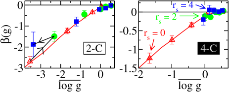
Figure 1: $\beta(g)$ as a function of $\overline{\log g}$ for the 2-C ($N$=32, left) and 4-C system ($N$=64, right). The red line is the non-interacting scaling function. Symbols stand for $r_{s}$=0 (triangles), $r_{s}$=2 (circles) and $r_{s}$=4 (squares), for $0.55<k_{F}l<24.5$. The black arrow in the left panel follows a given value of disorder for increasing $r_{s}$.

Let us start with the study of the $\beta(g)$ function, shown in Fig. 1. We do not assume that $\beta$ is a function of $g$ only, but we merely plot simultaneously $\beta=d\log g/d\log L$ and $g$ while varying both $k_{F}l$ and $r_{s}$. Upon switching on the interaction in the 2-C system, $g$ and $\beta$ first increase quickly. They reach a maximum at $r_{s}\approx 2$ and then decrease. We observe no visible deviation from one-parameter scaling: even though $g$ and $\beta$ increase with $r_{s}$, the trajectory $[g(r_{s}),\beta(r_{s})]$ remains on the non-interacting $\beta(g)$ curve. In particular, at $r_{s}\approx 2$ where the delocalisation effect is maximum, the value of $\beta$ always remains strictly negative $\beta<0$ so that, even though the localisation length $\xi$ has increased significantly, it is still finite, and the system would still be insulating in the thermodynamic limit. The situation for the 4-C system is qualitatively different from 2-C as the delocalisation effect is much more pronounced: $\beta$ quickly increases with $r_{s}$ and reaches $\beta=0$ i.e. a metallic state up to our statistical precision. While the non interacting points are spread over a wide range of $g$ and $\beta$, once the interaction is switched on, all the points (but one obtained for the strongest disorder) move toward $\beta=0$. Hence, the localisation length $\xi$ becomes much larger than the system size and the system becomes practically a metal. Yet, as in 2-C, we observe no visible deviation from one parameter scaling so that even though $\xi$ has increased dramatically we cannot conclude that the system becomes a “true” metal in the thermodynamic sense (i.e. a divergence of $\xi$). We note that indications that spin and valley degeneracy could play a positive role for transport properties were found in the limit of low disorder and interaction ($k_{F}l\rightarrow\infty$, $r_{s}\ll 1$) as early as 1983 Finkelshtein (1983); Castellani et al. (1984). However, these works predicted deviations from one parameter scaling which we did not observe in our (non-perturbative) regime of parameters ($0.5<k_{F}l<4$ , $0\leq r_{s}\leq 10$).

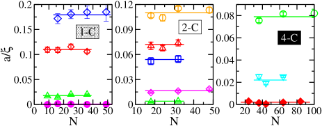
Figure 2: $a/\xi$ as a function of $N$ for 1-C (left), 2-C (middle) and 4-C systems (right panel). The symbols correspond to different strengths of interaction ($r_{s}=0$ (circles), $r_{s}=0.25$ (down triangles), $r_{s}=2$ (diamonds), $r_{s}=4$ (up triangles) and $r_{s}=6$ (squares)) and of disorder ($1<k_{F}l<6$ for 1-C, $1<k_{F}l<2.4$ for 2-C and $k_{F}l=1.05$ for 4-C).

As we observed no deviation to one parameter scaling, it means that all the relevant information of the system is encapsuled in the (one parameter) localization length $\xi(r_{s},k_{F}l)$ of the system. Integrating the $\beta(g)=d\log g/d\log L$ function, one parameter scaling implies that

$$\frac{1}{\xi}\equiv\frac{1}{L}\exp\int_{-1.5}^{\log g}\frac{d\log u}{\beta[\log u]}$$ (2)

is independent of the size of the system. We have carefully tabulated $\beta(g)$ without interaction and we use Eq.(2) to extract $\xi$. Note that even if there are deviations from the non-interacting $\beta(g)$, those are small in the regime of parameters that we have considered, and can be safely ignored for our purpose. We also emphasize that this method allow us to extract $\xi$ even when $\xi\approx L$ and that we recover $g=g_{0}e^{-L/\xi}$ for $L\gg\xi$. In Fig. 2, we plot $a/\xi$ as a function of $N$ for various values of disorder and interaction ($a\equiv 1/\sqrt{\pi\nu}$ is the averaged distance between particles). Except for very small $N$ (not shown), we find that $a/\xi$ is indeed independent of $N$ for all three systems 1-C, 2-C and 4-C. Note that for 4-C, we show only one value of $k_{F}l$ for different $r_{s}=0$, $r_{s}=0.25$ and $r_{s}=2$. For the latter, $a/\xi=0$ up to our statistical resolution while the corresponding non-interacting system is localized. Hence, the observed (strong) delocalization effect is robust against increasing $N$.

The corresponding localization lengths have been collected in Fig. 3 which is the chief result of this letter. It is, to the best of our knowledge, the first calculation of the localisation length in presence of many-body correlations.

In the rest of this letter, we turn to the implications of these results to the transport properties of 2D gases. A strong debate has taken place in the literature on the nature of the observed metallic behaviour Kravchenko et al. (1994) (i.e. decrease of resistivity as temperature is lowered). We will argue that the above findings provide a simple mechanism that accounts for the main experimental observations.

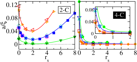
Figure 3: Inverse localisation length $a/\xi(r_{s})$ for the 2-C (left) and 4-C systems (right) at various $N$ and $k_{F}l$. For 2-C: top to bottom: $k_{F}l$=1.05 ($N$=32 left triangles, $N$=24 right triangles), $k_{F}l$=1.51 ($N$=32 diamonds, $N$=24 circles, $N$=18 squares), $k_{F}l$=2.36 ($N$=32 up triangles, $N$=18 down triangles). For 4-C: $k_{F}l$=0.77 ($N$=36 circles), $k_{F}l=1.05$ ($N$=84 cross, $N$=64 down triangles, $N$=36 up triangles), $k_{F}l$=1.51 ($N$=64 squares, $N$=36 diamonds). Inset: zoom of the main figure. Lines are guides to the eye. Error bars are roughly equal to symbols sizes.

The first observation of importance in those low density systems, is that the Fermi energy is extremely low, so that the actual typical temperature is not much smaller than the Fermi temperature. This is to be contrasted with more conventional systems where only a small fraction of the electrons around the Fermi surface take part in the transport properties. Hence, the nature of the (highly) excited states and in particular their localisation properties is of crucial importance here. In a non-interacting system, the localization length varies very quickly with $k_{F}l$ as electrons gather kinetic energy, typically exponentially Lee and Ramakrishnan (1985). An immediate consequence is that the excited states, with higher kinetic energy, are less localized than the ground state. In particular, the polarized system is less localized than the (non polarized) ground state. In such a situation, one naturally expects a negative in plane magnetoresistance: an in plane magnetic field $H$ (with no orbital but only Zeeman coupling to the electrons) polarizes the system hence delocalizes the system whose resistance decreases. Similarly, upon increasing the temperature $T$, the less localized excited states get populated and the overall resistance decreases.

Now, we find that this natural order can be reversed in presence of interactions. One ends up in a situation where the ground state is delocalized while its excited states are still strongly localized. In this situation, the behaviour of the resistivity upon increasing an in plane magnetic field $H$ or the temperature is reversed with respect to the non-interacting case: populating the highly localized excited states leads to an increase of resistivity, hence a positive in plane magnetoresistance as well as an increase of resistance upon increasing temperature (as in the “metallic” phase of the Si MOSFETs). Both effects are expected to take place when the corresponding Zeeman energy ${\rm g}\mu_{B}H/2$ and temperature $kT$ are of the order of the characteristic energy on which $\xi$ varies, i.e. the energy $E_{P}(k_{F}l,r_{s})$ to polarize the system.

In the “phase diagram” Fig. 4, we have plotted the difference $\delta\equiv a/\xi_{NP}-a/\xi_{P}$ of the inverse localization length for the non-polarized $\xi_{NP}$ and polarized $\xi_{P}$ systems. The polarized system is an excited state of the non polarized one, and we have verified numerically that the picture that follows also apply to partially polarized systems (excited states of lower energy). The $(r_{s},k_{F}l)$ plane can be divided into three regions. In the white region $k_{F}l\geq 4$, both localization lengths $\xi_{P}$ and $\xi_{NP}$ are extremely large so that $\delta$ is essentially zero. Upon increasing disorder $k_{F}l<4$ at small $r_{s}$, the localization length of the system decreases quickly. Yet, as the interaction is weak, the polarized system is less localized than the non-polarized one which leads to a positive $\delta$ (red, $+$). In the last region (blue, $-$), the interaction have delocalized the non-polarized system much more than the polarized one, hence a negative $\delta$. In our view, this (new) blue region corresponds to the regime where the metallic behaviour has been observed. Note that there is an important difference between 2-C and 4-C in the blue region: for 4-C, the ground state is (for practical purposes) delocalized while for 2-C it is not. Hence, for 2-C, temperature has two conflicting effects: on one hand it activates transport mechanisms such as variable range hopping Efros and Shklovskii (1975), while on the other hand it populates the (more localized) excited states.

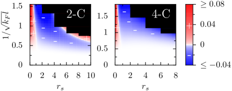
Figure 4: $\delta(r_{s},1/\sqrt{k_{F}l})$ for the 2-C (left) and 4-C system (right panel). $\delta>0$ (red, $+$) indicates that the polarized system is less localized than the non-polarized one, $\delta<0$ (blue, $-$) the opposite. No data are available in the black regions.

Upon varying density, a given sample moves on Fig. 4 according to $r_{s}=\eta/\sqrt{k_{F}l}$ (straight lines). In the absence of interaction, $\eta=2\sqrt{\mu}e^{3/2}m^{*}/(\hbar^{3/2}\epsilon\sqrt{M})$, so that the mobility $\mu$ obtained at low temperature and large density (small interaction) can be used as an estimate of $\eta$. We note however that upon varying density, $\eta$ remains constant only for white disorder. Real disorder is correlated so that $\eta$ is expected to increase at low density as larger scales are probed. Also, the disorder seen by the electrons at the Fermi level is partially screened by the rest so that the above formula overestimates $\eta$. Rough estimates are $\eta\approx 10$ (high mobility Si MOSFET, $\mu\geq 10^{4}{\rm cm^{2}.V^{-1}.s^{-1}}$), $\eta\approx 50$ (electrons in GaAs/GaAlAs heterostructures, $\mu\geq 10^{6}{\rm cm^{2}.V^{-1}.s^{-1}}$), and $\eta\approx 200$ (holes in GaAs/GaAlAs heterostructures, $\mu\approx 10^{6}{\rm cm^{2}.V^{-1}.s^{-1}}$) so that high mobility Si MOSFETs are dirtier than their III-V counterparts.

For definiteness, let us concentrate on the data presented in Fig.1 of Ref. Altshuler et al. (2000) (hereafter referred as Fig.A) for a typical high mobility Si MOSFET. At very high density ($k_{F}l\gg 1$, $r_{s}\ll 1$), the system can be described within diagrammatic theory which predicts small quantum corrections to transport properties Lee and Ramakrishnan (1985). This is the left part of the white region in Fig. 4 where one observes, for instance, the usual signatures of weak localization. The resistivity $\rho(T)$ as a function of temperature is roughly flat in this region (except at large temperature where phonons set in). Upon decreasing the density, one enters the blue region of Fig. 4 at $k_{F}l\approx 4$ ($n_{s}\approx 2.5\ 10^{11}{\rm cm^{-2}}$ for the sample of Fig. A). In this region, one observes the strong positive variation of $\rho(T)$ which has been puzzling the community for more than a decade. We attribute this behaviour to the fact that in this region, the ground state is (for all practical purposes) delocalized (see right panel of Fig. 3) while its excitations are not. Hence upon increasing temperature those localized states get populated and the resistivity increases strongly. This scenario implies in particular that (i) The corresponding characteristic energy scale where the increase of $\rho(T)$ is expected is the energy $E_{P}(k_{F}l,r_{s})$ to polarize the system. We have calculated numerically this energy scale in the relevant regime and found $E_{P}\approx 0.15E_{F}$ where $E_{F}$ is the Fermi energy. Indeed, one observes in Fig. A that $T/T_{F}\approx 0.15$ corresponds to the crossover temperature where the strong increase of $\rho(T)$ takes place. (ii) An in plane magnetic field polarizes the system which becomes localized, hence a positive magnetoresistance is expected with a variation of resistance of the same order of magnitude as the variation due to the change in temperature. This is indeed observed for magnetic fields $H$ that correspond to a Zeeman energy of the order of $E_{P}$ (i.e. $\approx 1.6T$ at $n_{s}=10^{11}{\rm cm^{-2}}$) as can be seen, for instance, in Fig.10 of Ref.Abrahams et al. (2001).

To conclude, we have reported on the first quantitative calculation of the localization length in an interacting two dimensional electronic gas. The scenario that naturally emerges from the data captures all the essential features of the experiments at a semi-quantitative level, with no adjustable parameters. In particular, our data account for: (i) why the metallic behaviour is found at low density, i.e. when the corresponding polarized system lies in the vicinity of the quantum of conductance. (ii) Why it is destroyed by an in plane magnetic field. (iii) Why Si MOSFETs, with valley degeneracy, show a much stronger metallic behaviour than other materials. (iv) Why disorder matters, and samples with $\eta<1$ will not exhibit the metallic behaviour (red part of Fig. 4) while too clean samples (white part) will only show a weak signal. (v) The characteristic magnetic field and temperature for the dependance of the resistivity.

We have not discussed the metal-insulator transition per se, but rather focused on the existence of the metallic behaviour. Indeed, for large interaction $r_{s}$ and disorder $1/k_{F}l$, there is no question that the system will eventually become insulating. Although the nature of this insulator and of the corresponding transition is clearly an interesting topic, the real mystery lies in the nature of the metal itself. Our results suggest that this metallic behaviour is due to a non-perturbative interaction delocalization effect. On the other hand, we found no significant deviation from the non-interacting one-parameter scaling which suggests that the 4-C systems are not “true” thermodynamic metals and would become insulating at ultrasmall temperature (2-C systems are unambiguously insulators). In any case, we find that the question of the existence of a “true” metal is not relevant in those experiments as a different physics (of much higher energy) has been probed in practice.