Constraints on $w_{0}$ and $w_{a}$ of Dark Energy from High Redshift Gamma Ray Bursts

Abstract

We extend the Hubble diagram up to $z=5.6$ using 63 gamma-ray bursts (GRBs) via peak energy-peak luminosity relation (so called Yonetoku relation), and obtain constraints on cosmological parameters including dynamical dark energy parametrized by $P/\rho\equiv w(z)=w_{0}+w_{a}\cdot z/(1+z)$. It is found that the current GRB data are consistent with the concordance model, ($\Omega_{m}=0.28,\Omega_{\Lambda}=0.72,w_{0}=-1,w_{a}=0$), within two sigma level. Although constraints from GRBs themselves are not so strong, they can improve the conventional constraints from SNeIa because GRBs have much higher redshifts. Further we estimate the constraints on the dark-energy parameters expected by future observations with GLAST (Gamma-ray Large Area Space Telescope) and Swift by Monte-Carlo simulation. Constraints would improve substantially with another 150 GRBs.

1 Introduction

In our previous paper (Kodama et al., 2008), we calibrated the peak energy-peak luminosity relation of GRBs with 33 nearby events ($z<1.62$) whose luminosity distances were estimated from those of large amount of SNeIa (Riess et al., 2007; Wood-Vasey et al., 2007; Davis et al., 2007). This calibrated Yonetoku relation, derived without assuming any cosmological models, can be used as a new cosmic distance ladder toward higher redshifts. Then we determined the luminosity distances of 30 GRBs in $1.8<z<5.6$ using the calibrated relation and calculated the likelihood varying $(\Omega_{m},\Omega_{\Lambda})$. We obtained $(\Omega_{m},\Omega_{\Lambda})=(0.37^{+0.14}_{-0.11},0.63^{+0.11}_{-0.14})$ for a flat universe, which is consistent with the concordance cosmological model within one sigma level. Our logic to obtain a new distance ladder is similar to that for SNeIa, that is, we calibrate a new distance indicator (Yonetoku relation) at low redshifts ($z<1.62$) using the well established indicators (SNeIa). Then we assume the new relation holds at high redshifts ($z>1.62$), although more detailed analysis is needed for possible selection bias and evolution effects in the relation (Oguri & Takahashi, 2006).

Currently the number of GRBs with $z>1.62$ is relatively small ($\sim 30$) and the statistical and systematic errors of the Yonetoku relation are not so small compared with SNeIa. Even then, GRBs are still effective to probe dark energy, especially for dynamical dark energy whose energy density becomes large at high redshifts, because the mean redshift of GRBs is higher than that of SNeIa (Amati et al., 2008; Liang et al., 2008; Basilakos & Perivolaropoulos, 2008; Schaefer, 2007; Ghirlanda et al., 2006; Firmani et al., 2006). There would be many ways to characterize the time variation of dark energy. Here we adopt a simple phenomenological model as (Chevallier & Polarski, 2001; Linder, 2003) $P/\rho\equiv w(z)=w_{0}+w_{a}\cdot z/(1+z)=w_{0}+w_{a}(1-a)$, where $w_{0}$ and $w_{a}$ are constants and $a$ is the scale factor of the universe. For this model, GRBs would give strong constraints on $w_{a}$ which represents the time dependence of dark energy.

In this Letter, we present constraints on cosmological parameters such as $w_{0}$ and $w_{a}$ using both SNeIa with $z<1.8$ and GRBs with $z<5.6$. In § 2, we briefly review the main results of the previous paper (Kodama et al., 2008) and the theoretical and observational basis of the analysis. In § 3-1, we assume cosmological constant ($w=-1$) and obtain constraints on ($\Omega_{m},\Omega_{\Lambda}$). In § 3-2, we assume a flat universe and non-dynamical ($w_{a}=0$) dark energy and obtain constraints on $(w_{0},\Omega_{m})$. In § 3-3, we fix $\Omega_{m}=0.28$ for simplicity, and obtain the plausible values of $w_{0}$ and $w_{a}$. In § 4, we discuss how these constraints will be improved in future observations of high redshift GRBs by such as GLAST. Throughout the paper, we fix the current Hubble parameter as $H_{0}=66~{}{\rm km~{}s^{-1}Mpc^{-1}}$.

2 Friedmann universe

In our previous paper (Kodama et al., 2008), we calibrated the Yonetoku relation (Yonetoku et al., 2004) using 33 events with the redshift $z<1.62$ as

$$(\frac{L_{p}}{10^{52}{\rm erg~{}s^{-1}}})=(1.31\pm 0.67)\times 10^{-4}(\frac{E_{p}}{\rm 1keV})^{1.68\pm 0.09},$$ (1)

where $L_{p}$ and $E_{p}$ are the peak luminosity and the peak energy of the spectrum of a certain GRB event in a comoving frame, respectively. Fig. 1 of the previous paper shows that the linear correlation coefficient of the above relation in logarithmic scale is 0.9478 and the chance probability is $6.0\times 10^{-17}$. However the data distribution has a larger deviation around the best fit line compared with the expected Gaussian distribution. We estimated this systematic deviation in the normalization as $9.57\times 10^{-5}$.

Now if one assumes that the above relation holds even for $z>1.8$, we can determine the luminosity distance $d_{L}(z)$ from the observed peak flux ($f_{p,{\rm obs}}$) and the observed peak energy of the spectrum $E_{p,{\rm obs}}$ since $L_{p}=4\pi d_{L}(z)^{2}f_{p,{\rm obs}}$ and $E_{p}=(1+z)E_{p,{\rm obs}}$. We express unknown equation of state of dark energy as $P=w_{X}(z)\rho$ and $\Omega_{X}$ as the present energy density of the dark energy divided by the critical density. Then in the Friedmann universe with $\Omega_{k}\equiv\Omega_{m}+\Omega_{X}-1$, the luminosity distance is given by

$${d_{L}^{\rm th}}(z,\Omega_{m},\Omega_{X},w)\!$$

$$~{}~{}~{}=\!\left\{\begin{array}[]{ll}\frac{c}{H_{0}\sqrt{\Omega_{k}}}\sin(\sqrt{\Omega_{k}}F(z))&\mbox{if}~{}~{}\Omega_{k}>0\\ \frac{c}{H_{0}\sqrt{-\Omega_{k}}}\sinh(\sqrt{-\Omega_{k}}F(z))&\mbox{if}~{}~{}\Omega_{k}<0\\ \frac{c}{H_{0}}F(z)&\mbox{if}~{}~{}\Omega_{k}=0\\ \end{array}\right.$$ (5)

with

$$F(z) = \int_{0}^{z}dz^{\prime}\,\Big{[}\Omega_{m}(1+z^{\prime})^{3}-\Omega_{k}(1+z^{\prime})^{2}$$ (6)

$$+\Omega_{X}e^{3\int_{0}^{\ln(1+z^{\prime})}d\ln(1+z^{\prime\prime})[1+w(z^{\prime\prime})]}\Big{]}^{-1/2}.$$

Using the distance modulus ($\mu_{0}(z_{i})$) from observation of SNeIa and GRBs, we define a likelihood function as

$$\Delta\chi^{2}=\sum_{i}\left\{\frac{\mu_{0}({z_{i}})-\mu^{\rm th}(z_{i},\Omega_{m},\Omega_{X},w)}{\sigma_{\mu_{0,z_{i}}}}\right\}^{2}-\chi_{\rm best}^{2},$$ (7)

where $\mu^{\rm th}(z_{i},\Omega_{m},\Omega_{X},w)=5\log(d_{L}^{\rm th}/{\rm Mpc})+25$ and $\chi_{\rm best}^{2}$ represents the chi-square value for the best fit parameter set of $\Omega_{m}$, $\Omega_{X}$ and $w$.

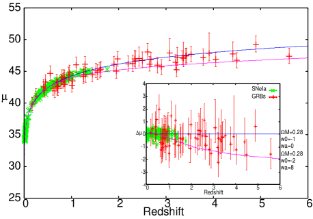
Figure 1: Hubble diagram extended to $z=5.6$ from GRBs. The green points and red points are the luminosity distance determined by SNeIa (Riess et al., 2007) and GRBs (Kodama et al., 2008), respectively. The blue line is the luminosity distance of $\Lambda$CDM model with ($\Omega_{m}$,$\Omega_{\Lambda}$)=(0.27,0.73). Inset figure is residual Hubble diagram and models after subtracting model ($\Omega_{m},$,$\Omega_{\Lambda}$)=(0.27,0.73). The pink line is the luminosity distance of the dynamical dark energy equation of state model with ($w_{0}$, $w_{a}$)=(-2, 8) discussed in § 3-3

3 cosmological parameters

Fig. 1 shows the Hubble diagram extended to $z=5.6$ by GRBs. The green points and red points are the luminosity distance determined by SNeIa (Riess et al., 2007; Wood-Vasey et al., 2007; Davis et al., 2007) and GRBs (Kodama et al., 2008), respectively. The blue and pink lines are the luminosity distances of $\Lambda$CDM model with ($\Omega_{m}$, $\Omega_{\Lambda}$)=(0.27, 0.73) and dynamical dark energy model with ($w_{0}$, $w_{a}$)=(-2, 8), respectively.

3.1 $\Lambda$CDM model

We first consider the cosmological constant model, that is $w_{0}=-1$ and $w_{a}=0$. Then Eq. (6) becomes

$$F(z)=\int_{0}^{z}\frac{dz}{\sqrt{\Omega_{m}(1+z)^{3}+\Omega_{\Lambda}-\Omega_{k}(1+z)^{2}}},$$ (8)

and $\chi^{2}$ is a function of ($\Omega_{m},\Omega_{\Lambda}$). Fig. 2 shows confidence regions for ($\Omega_{m},\Omega_{\Lambda}$) from 63 GRBs (light blue dash-dotted lines), 192 SNeIa (blue dotted lines), and 63 GRBs + 192 SNeIa (red solid lines), respectively. Without any prior the set of the cosmological parameters with the largest likelihood is ($\Omega_{m}$,$\Omega_{\Lambda}$) = ($0.38_{-0.09}^{+0.09}$,$0.93_{-0.15}^{+0.14}$) with $\chi_{\rm best}^{2}=225.2/253$.

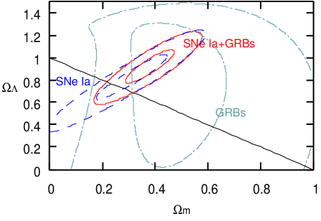
Figure 2: The contours of likelihood $\Delta\chi^{2}$ in ($\Omega_{m}\-\Omega_{\Lambda}$) plane for GRBs (light blue dash-doted lines), SNeIa(blue dotted lines), SNeIa + GRBs (red solid lines), respectively. The contours correspond to 68.3% and 99.7% confidence regions, respectively, and black solid line represents the flat universe. The shape of GRB contour is more vertical because GRBs have higher redshifts.

3.2 non-dynamical dark energy model

In this section we assume a flat universe with $w_{a}=0$. Then

$$F(z)=\int_{0}^{z}\frac{dz}{\sqrt{\Omega_{m}(1+z)^{3}+(1-\Omega_{m})(1+z)^{3(1+w_{0})}}},$$ (9)

and the likelihood function depends on $\Omega_{m}$ and $w_{0}$. Fig. 3 shows the likelihood contours on ($\Omega_{m},w_{0}$) plane for GRBs (light blue dash-dotted lines), SNeIa (blue dotted lines), SNeIa + GRBs (solid red lines), respectively. The contours correspond to 68.3% and 99.7% confidence regions, respectively. The set of the cosmological parameters with the largest likelihood is ($\Omega_{m}$, $w_{0}$) = ($0.36_{-0.11}^{+0.08}$, $-1.33_{-0.15}^{+0.48}$) with $\chi_{\rm best}^{2}=227.0/253$.

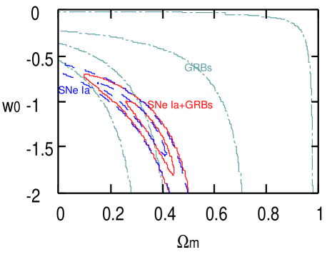
Figure 3: The contours of likelihood of $\Delta\chi^{2}$ in ($\Omega_{m}$, $w_{0}$) plane for GRBs (light blue dash-dotted lines), SNeIa (blue dotted lines), SNeIa + GRBs (red solid lines), respectively. The contours correspond to 68.3% and 99.7% confidence regions, respectively.

3.3 Dynamical dark energy model

As already shown, we adopt the parameterization of $w(z)$ as (Chevallier & Polarski, 2001; Linder, 2003)

$$w(z)=w_{0}+w_{a}(1-a)=w_{0}+w_{a}\frac{z}{1+z}.$$ (10)

This is not the only parameterization and, for example, $w(z)=w_{0}+w_{1}z$ can be found in the literature. However, $w(z)$ is diverging for large $z$ in this ($w_{0},w_{1}$) parameterization, which would not be appropriate for our high redshift GRB samples. Now Eq. (6) becomes

$$F(z) = \int_{0}^{z}dz\,\Big{[}\Omega_{m}(1+z)^{3}$$ (11)

$$(1-\Omega_{m})(1+z)^{3(1+w_{0}+w_{a})}e^{-3w_{a}\frac{z}{1+z}}\Big{]}^{-1/2}.$$

For simplicity, we fix $\Omega_{m}=0.28$. Fig. 4 shows the contours of likelihood $\Delta\chi^{2}$ in the ($w_{0}$, $w_{a}$) plane from GRBs (light blue dash-dotted lines), SNeIa (blue dotted lines), SNeIa + GRBs (red solid lines), respectively. The contours correspond to 68.3% and 99.7% confidence regions, respectively. The shape of probability contour is more horizontal than that of SNeIa, because of the higher redshift distribution of GRBs. The set of the dark-energy parameters with the largest likelihood is ($w_{0}$, $w_{a}$) = ($-1.26_{-0.32}^{+0.38},1.4_{-0.2}^{+1.8}$) with $\chi^{2}_{\rm best}=227.6/253$. The pink line in the inset of Fig. 1 is the model with ($w_{0},w_{a}$) = ($-2,8$) which is three sigma level from the best fit. We can see that this model does not fit the data by eyes.

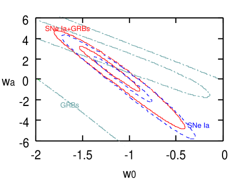
Figure 4: The contours of likelihood of $\Delta\chi^{2}$ in ($w_{0}$,$w_{a}$) plane for GRBs (light blue dash-doted lines), SNeIa (blue dotted lines), SNeIa + GRBs (red solid lines), respectively. The contours correspond to 68.3% and 99.7 % confidence regions, respectively.

Figs. 2, 3 and 4 show that the constraints on cosmological parameters from SNeIa are stronger than those from GRBs at present. However the shapes of the likelihood contours are different. In Figs. 2 and 3, the contours from GRBs are more vertical than that from SNeIa. This behaviour is clear from Eqs. (8) and (9). GRBs include higher redshifts up to $z=5.6$ at present so that the value of $F(z)$ is more sensitive on the value of $\Omega_{m}$. Therefore we can expect independent stronger constraints on cosmological parameters if the systematic error in Yonetoku relation decreases and/or the number of high redshift GRBs increases. Fig. 4 shows also that the contour from GRBs is more horizontal than SNeIa. Since the mean value of the redshift for SNeIa samples and GRB samples are 0.48 and 1.97, respectively, we see that GRBs should give more stronger constraints on $w_{a}$ from the exponential term in Eq. (11).

4 Future prospect of gamma-ray burst cosmology

In this section we investigate the future prospect of probing dark-energy parameters with GRBs. The Gamma-ray Large Area Space Telescope (GLAST) was launched June 11, 2008 and it would substantially increase the potential of GRBs as cosmological probes. In fact, due to the wide energy-band of GLAST Burst Monitor (GBM) and positional accuracy of Large Area Telescope (LAT), GLAST is expected to detect 30 GRBs/year with spectral peak energy and spectroscopic redshift by joint observation with Swift .

Here we estimate the accuracy of determination of the dark-energy parameters with GLAST by Monte-Carlo simulation. We generate 150 GRB events in the following way. First, GRBs are distributed in redshift-luminosity plane according to the GRB formation rate and luminosity function given by Porciani & Madau (2001). Spectral peak energy is assigned to each GRB according to the best-fit Yonetoku relation with intrinsic dispersion of $30\%$. Calculating the flux at the earth assuming the concordance model, a GRB is counted as an observed event if the flux exceeds the sensitivity of GLAST. For observed events, observational errors of $20\%$ are added to the observed flux and spectral peak energy. In this way, we generate 150 observed events and they are divided into two groups, high-redshift group (77 GRBs with $z>1.7$) and low-redshift group (73 GRBs with $z<1.7$). As we did with real GRB events, we reconstruct Yonetoku relation with low-redshift GRBs. With increased number of low-redshift events, the normalization and index of Yonetoku relation are determined with reduced errors of $5\%$ and $3\%$, respectively. Applying the reconstructed relation to high-redshift events, we can put them in the Hubble diagram and constrain the cosmological parameters. For the details of our Monte-Carlo method, see (Takahashi et al., 2003; Oguri & Takahashi, 2006).

Figs. 5 and 6 show the constraint in ($\Omega_{m},w_{0}$) and ($w_{0},w_{a}$) planes, respectively, from the “real + simulated” high-redshift GRBs (light blue dash-dotted lines), “real” SNeIa (blue dotted lines), and SNeIa + GRBs (red solid lines). The contours correspond to 68.3% and 99.7 % confidence regions, respectively. These figures indicate how GRBs can be a powerful probe to study the nature of dark energy.

In conclusion, the increase of high redshift GRB data by such as GLAST and Swift is indispensable to determine the time variation of the dark energy in $z>1.8$ where SNeIa data would be rare.

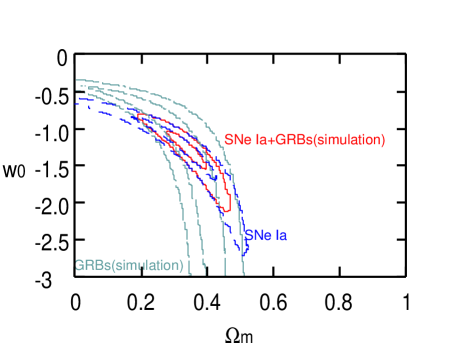
Figure 5: The contours of likelihood of $\Delta\chi^{2}$ in ($\Omega_{m}$,$w_{0}$) plane from the real + simulated GRBs (light blue dash-dotted lines), SNeIa (blue dotted lines), and SNeIa + GRBs (red solid lines), respectively. The contours correspond to 68.3% and 99.7 % confidence regions, respectively.

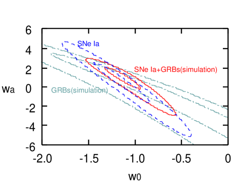
Figure 6: The contours of likelihood of $\Delta\chi^{2}$ in ($w_{0}$,$w_{a}$) plane from the real + simulated GRBs (light blue dash-dotted lines), SNeIa (blue dotted lines), and SNeIa + GRBs (red solid lines), respectively. The contours correspond to 68.3% and 99.7 % confidence regions, respectively.

References

- Amati et al. (2008) Amati, L., Guidorzi, C., Frontera, F., Della Valle, M., Finelli, F., Landi, R., & Montanari, E. 2008, ArXiv e-prints, 805, arXiv:0805.0377
- Basilakos & Perivolaropoulos (2008) Basilakos, S., & Perivolaropoulos, L. 2008, ArXiv e-prints, 805, arXiv:0805.0875
- Chevallier & Polarski (2001) Chevallier, M., & Polarski, D. 2001, International Journal of Modern Physics D, 10, 213
- Davis et al. (2007) Davis, T. M., et al. 2007, ApJ, 666, 716
- Firmani et al. (2006) Firmani, C., Avila-Reese, V., Ghisellini, G., & Ghirlanda, G. 2006, MNRAS, 372, L28
- Ghirlanda et al. (2006) Ghirlanda, G., Ghisellini, G., & Firmani, C. 2006, New Journal of Physics, 8, 123
- Kodama et al. (2008) Kodama, Y., Yonetoku, D., Murakami, T., Tanabe, S., Tsutsui, R., & Nakamura, T. 2008, MNRAS in press, arXiv:0802.3428
- Liang et al. (2008) Liang, N., Xiao, W. K., Liu, Y., & Zhang, S. N. 2008, ArXiv e-prints, 802, arXiv:0802.4262
- Linder (2003) Linder, E. V. 2003, Physical Review Letters, 90, 091301
- Oguri & Takahashi (2006) Oguri, M., & Takahashi, K. 2006, Physical Review D, 73, 123002
- Porciani & Madau (2001) Porciani, C., & Madau, P. 2001, ApJ, 548, 522
- Riess et al. (2007) Riess, A. G., et al. 2007, ApJ, 659, 98
- Schaefer (2007) Schaefer, B. E. 2007, ApJ, 660, 16
- Takahashi et al. (2003) Takahashi, K., Oguri, M., Kotake, K., & Ohno, H. 2003, ArXiv Astrophysics e-prints, arXiv:astro-ph/0305260
- Wood-Vasey et al. (2007) Wood-Vasey, W. M., et al. 2007, ApJ, 666, 694
- Yonetoku et al. (2004) Yonetoku, D., Murakami, T., Nakamura, T., Yamazaki, R., Inoue, A. K., & Ioka, K. 2004, ApJ, 609, 935