A jet model for Galactic black-hole X-ray sources: Some constraining correlations

Abstract

Context. Some recent observational results impose significant constraints on all the models that have been proposed to explain the Galactic black-hole X-ray sources in the hard state. In particular, it has been found that during the hard state of Cyg X-1 the power-law photon number spectral index, $\Gamma$, is correlated with the average time lag, $<t_{\rm lag}>$, between hard and soft X-rays. Furthermore, the peak frequencies of the four Lorentzians that fit the observed power spectra are correlated with both $\Gamma$ and $<t_{\rm lag}>$.

Aims. We have investigated whether our jet model can reproduce these correlations.

Methods. We performed Monte Carlo simulations of Compton upscattering of soft, accretion-disk photons in the jet and computed the time lag between hard and soft photons and the power-law index $\Gamma$ of the resulting photon number spectra.

Results. We demonstrate that our jet model naturally explains the above correlations, with no additional requirements and no additional parameters.

1 Introduction

The states of Galactic black-hole X-ray sources (GBHs) are determined from the following quantities: i) their disk fraction, which is the ratio of the disk flux to the total flux, both unabsorbed, at $2-20$ keV; ii) the photon number spectral index, $\Gamma$, of the hard band, power-law component at energies below any break or cutoff; iii) the root-mean-square (rms) power in the power spectral density (PSD) integrated from 0.1–10 Hz; iv) the integrated rms amplitude of any quasi-periodic oscillation (QPO) detected in the range 0.1–10 Hz (Remillard & McClintock 2006). In particular, the so-called hard state is characterized by a power-law X-ray spectrum with photon number spectral index $1.5\mathbin{\lower 3.0pt\hbox{$\hbox to0.0pt{\raise 5.0pt\hbox{$\char 60\relax$}\hss}\mathchar 29208\relax$}}\Gamma\mathbin{\lower 3.0pt\hbox{$\hbox to0.0pt{\raise 5.0pt\hbox{$\char 60\relax$}\hss}\mathchar 29208\relax$}}2.1$, which suffers an exponential cutoff at $\sim$ 100 or few 100 keV, and contributes more than 80% of the 2–20 keV flux.

Several models have succeeded in reproducing the observed X-ray spectrum in this state (see e.g. Titarchuk 1994; Esin et al. 1997; Poutanen & Fabian 1999; Reig et al. 2003; Giannios et al. 2004). When a GBH is in the hard state, radio emission is also detected and a jet is either seen or inferred (Fender 2001). Again, several models are successful in reproducing the energy spectrum from the radio domain to the hard X-rays (see e.g. Markoff et al. 2001; Vadawale et al. 2001; Corbel & Fender 2002; Markoff et al. 2003; Giannios 2005). The multiplicity of models that can fit the time average spectrum of GBHs well indicates that this alone is not enough to distinguish the most realistic among them.

Timing data of the observed intensity in various energy bands provide a totally different “dimension” than the spectral one, and can in principle provide information on the location, size, physical conditions and kinematics of the plasma responsible for the X-ray emission in these objects. For example, the X-ray light curves of GBHs in different energy bands show similar variations, but those in the higher energy band generally lag the variations detected in the lower energy band (Nowak et al. 1999; Ford et al. 1999). The time delay, $t_{\rm lag}$, usually depends on frequency, $\nu$. For Cyg X-1 the time delays decrease with increasing frequency roughly as $t_{\rm lag}\propto\nu^{-\beta}$, where $\beta\approx 0.7$. As constraining as it is, this relation has also been explained in more than one way (see e.g. Poutanen & Fabian 1999; Reig et al. 2003; Körding & Falcke 2004).

Even more constraining to models is the fact that the high-frequency power spectrum flattens as the photon energy increases (Nowak et al. 1999). Equivalent to this is the fact that the width of the temporal autocorrelation function of the light curves of Cyg X-1 decreases with increasing photon energy (Maccarone et al. 2000). These observational facts are contrary to what one expects from simple Comptonization models, yet possible explanations for them have also been offered (Kotov et al. 2001; Giannios et al. 2004).

Significant advances in our understanding of how the X-ray mechanism in GBHs (and compact accreting objects in general) works can be achieved when we combine variability and spectral information. This has been possible in the last few years, due mainly to RXTE. For example, in the case of Cyg X-1, Pottschmidt et al. (2003) used 130 RXTE observations between 1998 and 2001 to study the long-term evolution of the source’s power and energy spectrum in detail. They used 512 s long light curves to estimate the power spectral density (PSD), which they fitted with a model that consisted of the sum of multiple Lorentzian profiles. They generally achieved good fits using four broad Lorentzian components with typical peak frequencies of $\nu_{1}\sim 0.2$ Hz, $\nu_{2}\sim 2$ Hz, $\nu_{3}\sim 6$ Hz, and $\nu_{4}\sim 40$ Hz, which vary in unison with time: their ratios remain constant despite each frequency varies by up to a factor of $\sim 5$. Up to now, no physical explanation of these Lorentzians has been offered. As for the energy spectrum, they find that a simple model consisting of a power-law component of index $\Gamma$, a multi-temperature disk black body and a reflection from neutral material component could fit the energy spectrum of the source below 20 keV.

They present convincing evidence that the timing and spectral properties of the source are closely linked. In fact, a number of the correlations they present impose stringent constraints on all the models proposed so far. These correlations are:

a) The observed photon number spectral index, $\Gamma$, correlates with the observed average time lag, $<t_{\rm lag}>$, between 2–4 keV and 8–13 keV, averaged over the 3.2–10 Hz frequency band, in the sense that $<t_{\rm lag}>$ increases as the spectrum steepens. Therefore, a model that can successfully explain the spectral slope $\Gamma$ should also predict the right amount of time delay between these specific energy bands and vice versa: a model that can fit well the time lag vs. Fourier frequency relation, should also predict the appropriate value of the index $\Gamma$ for a given time delay.

b) The observed photon number spectral index, $\Gamma$, also correlates with the Lorentzian peak frequencies: the frequencies increase as the spectrum steepens (see also Shaposhnikov & Titarchuk 2006, 2007).

In summary, the Pottschmidt et al. (2003) results show that a specific value of $\Gamma$, say $\Gamma=2$, which is relatively easy to obtain with a simple Comptonization model, must also be associated with specific values of the Lorentzian peak frequencies and a specific value of $<t_{\rm lag}>$! These are challenging relations that any model must be able to explain. In this work we investigate whether the jet model that we have proposed can meet these constraints under reasonable assumptions.

We think that the jets in GBHs play a central role in all the observed phenomena, not only in the radio emission. We have shown that Compton upscattering in the jet of soft photons from the accretion disk can explain: 1) the X-ray spectrum and the time-lag dependence on Fourier frequency (Reig et al. 2003, hereafter Paper I); 2) the narrowing of the autocorrelation function and the increase of the rms amplitude of variability with increasing photon energy (Giannios et al. 2004, hereafter Paper II); 3) the energy spectrum from radio to hard X-rays of XTE J1118+480, the only source for which we have simultaneous observations for all energy bands (Giannios 2005, hereafter Paper III).

In this paper we show that the jet model proposed and developed in the above work can explain the $\Gamma$ – $<t_{\rm lag}>$ relation of Pottschmidt et al. (2003), with no additional parameters or requirements, if we let just two model parameters, namely the radius at the base of the jet and the optical depth along its axis, vary over a reasonable range of values. At the same time, the model can also explain the ”$\Gamma$ – Lorentzian peak frequencies $\nu_{i}$” relation qualitatively if we identify $1/\nu_{i}$, $i=1,2,3,4$, with quantities proportional to the characteristic timescale $M_{\rm out}/{\dot{M}}_{\rm out}$, where ${\dot{M}}_{\rm out}$ is the rate of mass outflow in the jet and $M_{\rm out}$ the available mass to power the jet. Finally, the model parameter variations that are needed to explain the Pottschmidt et al. (2003) relations also predict that, on long time scales, the radio variations should also correlate with $\Gamma$, which, as we show, is indeed the case in Cyg X-1.

In Sect. 2 we describe briefly our model, in Sect. 3 we present and discuss our results, and we close with our conclusions in Sect. 4.

2 The model

The jet model used here is the same as the one described in Papers I, II and III. A summary is given below so that the reader becomes familiar with the parameters involved. First, we discuss the asumptions made in the model; then we describe how our Monte Carlo code works and finally we explain the meaning of the various parameters involved.

2.1 Description of the jet

We assume that the jet is accelerated close to its launching area and maintains a constant (mildly relativistic) bulk speed, $v_{\parallel}$, thereafter. The electron-density profile in the jet is taken to have the form

$$n_{\rm e}(z)=n_{0}(z_{0}/z),$$

where $z$ is the distance from the black hole perpendicular to the accretion disk. The parameters $n_{0}$ and $z_{0}$ are the electron density and the height of the base of the jet. The Thomson optical depth along the axis of the jet is

$${\tau}_{\parallel}=n_{0}{\sigma}_{T}z_{0}\ln(H/z_{0}),$$

where $H$ is the extent of the jet along the $z$ axis.

Let $\pi R^{2}(z)$ be the cross-sectional area of the jet as a function of height $z$. Then from the continuity equation ${\dot{M}}_{\rm out}=\pi R^{2}(z)m_{p}n_{e}(z)v_{\parallel}$, we obtain the radial extent $R$ of the jet as a function of height $z$

$$R(z)=R_{0}(z/z_{0})^{1/2}.$$

Here $R_{0}=({\dot{M}}_{\rm out}/\pi m_{p}n_{0}v_{\parallel})^{1/2}$ is the radius of the jet at its base, ${\dot{M}}_{\rm out}$ is the mass-outflow rate, $m_{p}$ is the proton mass, and $v_{\parallel}$ is the component of the velocity of the electrons parallel to the $z$ axis.

For computational simplicity, we assume that a uniform magnetic field exists along the axis of the jet (taken to be the $z$ axis). The $z$-dependence of the magnetic field is dictated by magnetic flux conservation along the jet axis to be

$$B(z)=B_{0}(z_{0}/z),$$

where $B_{0}$ is the magnetic field strength at the base of the jet. Also for computational simplicity we take the electrons’ velocity as having two components one parallel ($v_{\parallel}$) and one perpendicular ($v_{\perp}$) to the magnetic field. The magnitude and direction of $v_{\parallel}$ are fixed; so is the magnitude of $v_{\perp}$. However, the direction of $v_{\perp}$ is continuously changing, being always tangent to a circle in the perpendicular plane with respect to the magnetic field.

It has been shown (Paper III) that a power-law distribution of electron velocities in the rest frame of the flow gives nearly identical results. This is because the dominant contribution to the scatterings comes from the electrons that have the lowest velocity (or the lowest Lorentz $\gamma$ factor), due to the steep power law of electron $\gamma$’s required to explain the overall spectrum.

2.2 The Monte Carlo simulations

For our Monte Carlo simulations we used the same code as in Paper I. The code has been checked with an independent code that was used in Papers II and III. The procedure we follow is described briefly below.

Photons from the inner part of the accretion disk, in the form of a blackbody distribution of characteristic temperature $T_{\rm bb}$, are injected at the base of the jet with an upward isotropic distribution. Each photon is given a weight equal to unity (equivalently, beam of flux unity) when it leaves the accretion disk, and its time of flight is set equal to zero. The optical depth $\tau(\hat{n})$ along the photon’s direction $\hat{n}$ is computed and a fraction $e^{-\tau(\hat{n})}$ of the photon’s weight escapes and is recorded. The rest of the weight of the photon gets scattered in the jet. If the effective optical depth in the jet is significant (i.e., $\mathbin{\lower 3.0pt\hbox{$\hbox to0.0pt{\raise 5.0pt\hbox{$\char 62\relax$}\hss}\mathchar 29208\relax$}}1$), then a progressively smaller and smaller weight of the photon experiences more and more scatterings. When the remaining weight in a photon becomes less than a small number (typically $10^{-8}$), we start with a new photon.

The time of flight of a random walking photon (or more accurately of its remaining weight) gets updated at every scattering by adding the last distance traveled divided by the speed of light. For the escaping weight along a travel direction, we add an extra time of flight outside the jet in order to bring in step all the photons (or fractions of them) that escape in a given direction from different points on the “surface” of the jet. The longer a fractional photon stays in the jet, the more energy it gains on average from the circular motion (i.e., $\@vec{v_{\perp}}$) of the electrons. Such Comptonization can occur everywhere in the jet. Yet, a photon that random walks high up in the jet has a longer time of flight than a photon that random walks near the bottom of the jet. The optical depth to electron scattering, the energy shift, and the new direction of the photons after scattering are computed using the corresponding relativistic expressions.

If the defining parameters of a photon (position, direction, energy, weight, and time of flight) at each stage of its flight are computed, then we can determine the spectrum of the radiation emerging from the scattering medium and the time of flight of each escaping fractional photon. The time of flight of all escaping fractional photons is recorded in 8192 time bins of 1/128 s each. In this way, we can compute the number of photons that are emitted by the jet in each time bin and for any energy band. In other words, we can create 64 s long light curves for any energy band, which correspond to the resulting emission of the jet in response to an instantaneous burst of soft photons that we assume enter the jet simultaneously.

Having created light curves in various energy bands, we can now compute delays between any pair of bands. In our case, we consider the light curves of the energy bands 2–4 and 8–14 keV (identical to the energy bands of the light curves that Pottschmidt et al. 2003 used). Following Vaughan & Nowak (1997), we compute the phase lag and, through it, the time lag between the two energy bands as a function of Fourier frequency (same as in Paper I). Then we compute the average time lag, $<t_{\rm lag}>$, in the Fourier frequency range 3.2–10 Hz (like Pottschmidt et al. 2003).

2.3 Parameter values

Our jet model has a number of free parameters, which are the same as in Paper I: the temperature $T_{bb}$ of the soft photon input, the extent $H$ of the jet, the radius $R_{0}$ and the height $z_{0}$ of the base of the jet, the Thomson optical depth ${\tau}_{\parallel}$ along the axis of the jet, the parallel component of the velocity $v_{\parallel}$ of the electrons, and the perpendicular velocity component $v_{\perp}$.

We note here that, due to the mildly relativistic flow in the jet, the emerging X-ray spectra from the jet depend on the angle between the line of sight and the magnetic field direction. In order to have good statistics in our Monte Carlo results, we combined all the escaping photons with directional cosine with respect to the axis of the jet in the range $0.2<\cos\theta<0.6$. Strictly speaking, this is inconsistent with our assumption of a uniform magnetic field. If the magnetic field and the bulk flow were uniform, then only one value of $\cos\theta$ would be appropriate for each source. As discussed in Paper II, a range of directional cosines is absolutely necessary for reproducing the observed phenomena. Therefore, a non-uniform (probably a spiraling) magnetic field permeates the jet and this, together with the bulk flow, result in the above range of directions. A range of directions is thus important, but the actual values of this range are not.

The values of the model parameters are chosen so that all the results of Papers I, II, and III (apart from the radio emission) are reproduced, and at the same time the hard band power-law component has a slope of $\Gamma=2.1$ while the average time lag, in the range 3.2–10 Hz, between the 2–4 keV and 8–14 keV bands is 5 ms (as observed by Pottschmidt et al. 2003). We call these values the reference values and they are: $kT_{\rm bb}=0.2$ keV, $H=10^{5}r_{g}$, $R_{0}=50r_{g}$, $z_{0}=5r_{g}$, $\tau_{\parallel}=3$, $v_{\parallel}=0.8c$, and $v_{\perp}=0.4c$, where $r_{g}=GM/c^{2}=1.5\times 10^{6}$ cm stands for the gravitational radius of a 10 solar-mass black hole.

In Fig. 1 we show the emerging X-ray spectrum for the reference values of the parameters. The spectrum above $\sim 2$ keV can be well-fitted with a power law with an exponential cutoff

$$dN/dE\propto E^{-\Gamma}\rm e^{-E/E_{\rm cut}},$$

where $\Gamma=2.1$ and $E_{\rm cut}=70$ keV. One can also see the soft X-ray spectrum (below $\sim 2$ keV), which is essentially the unscattered part of the soft-photon input.

Figure 1: Emergent photon-number spectrum multiplied by $E^{2}$ from our jet model for the reference values of the parameters given in Sect. 3. The soft X-ray excess below $\sim$ 2 keV is essentially the unscattered soft-photon input. When fitted with a power law with an exponential cutoff (see Eq. 5), we find $\Gamma=2.1$ and $E_{\rm cut}=70$ keV.

3 Results and discussion

3.1 The spectral index – time lag relation

Our first aim is to investigate whether we can reproduce the $\Gamma$ - $<t_{\rm lag}>$ correlation of Pottschmidt et al. (2003, see their Fig. 7c) by allowing only a few model parameter values to change by a “reasonable amount” around their reference values.

It was shown in Paper II that keeping the rest of the parameters to their reference values and increasing $n_{0}$ (or equivalently the Thomson optical depth along the axis of the jet $\tau_{\parallel}$) makes the emergent spectra harder (the photons are scattered more often and gain more energy from the energetic electrons of the jet). Similarly, by increasing $R_{0}$, the spectrum hardens. This is because a larger $R_{0}$ translates to a larger Thomson optical depth perpendicular to the jet axis (we kept the rest of the parameters at their reference values) and therefore more photon scatterings. At the same time, time lags should also depend on the dimensions of the jet and its Thomson depth.

Thus, since both $R_{0}$ and $n_{0}$ affect the slope of the continuum and the time lags, it seems reasonable to run a series of models with only $R_{0}$ and $n_{0}$ varying, while the rest of the parameters of the model are kept fixed at their reference values. For $R_{0}$, we considered the values between 12 and 110 $r_{g}$ (with a step of $\Delta R_{0}=2$), while, for each $R_{0}$, $\tau_{\parallel}$ was left free to vary between 1 and 10, with a step of $\Delta\tau_{\parallel}=0.2$ (we discuss the model results in terms of $\tau_{\parallel}$, rather than $n_{0}$, because it is more informative about the average number of scatterings that each photon has suffered). For each run, i.e., each pair ($R_{0}$, $\tau_{\parallel}$), we derived the photon index $\Gamma_{\rm model}$ from a fit to the emergent spectrum between 2 and 20 keV (i.e., with no exponential cutoff, and thus with a slightly different $\Gamma$ from that of Eq. 5) and the average time lag, $<t_{\rm lag,model}>$, as explained in Sect. 2.2.

In Fig. 2 we represent the $\Gamma-<t_{\rm lag}>$ relation of Pottschmidt et al. (2003) (i.e. the observations), while Fig. 3 shows the input model parameters ($R_{0}$, $\tau_{\parallel}$) that generate the points ($\Gamma_{\rm model},<t_{\rm lag,model}>$) of Fig. 2. We show only those model results that agree best with the observed points. We find that the model can reproduce well the observed $\Gamma-<t_{\rm lag}>$ relation in Cyg X-1 if the radius at the base of the jet and the optical depth along the jet axis vary between $R_{0}\approx 5$ and 50 Schwarzschild radii, $r_{s}$ ($r_{s}=2r_{g}$), and $\tau_{\parallel}\approx 1.5-10$, respectively.

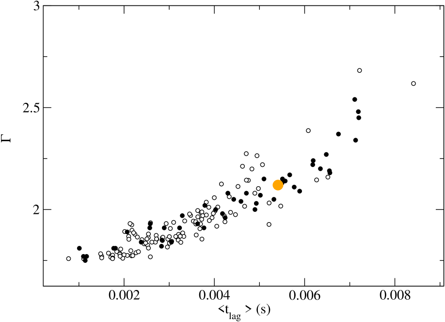
Figure 2: Correlation between the photon number spectral index $\Gamma$ and the average time lag $<t_{\rm lag}>$ between 2 - 4 keV and 8 - 14 keV in the frequency range 3.2 - 10 Hz. Empty circles are from Pottschmidt et al. (2003) and filled circles are the results of our model. The larger grey circle represents the model with the reference values of the parameters.

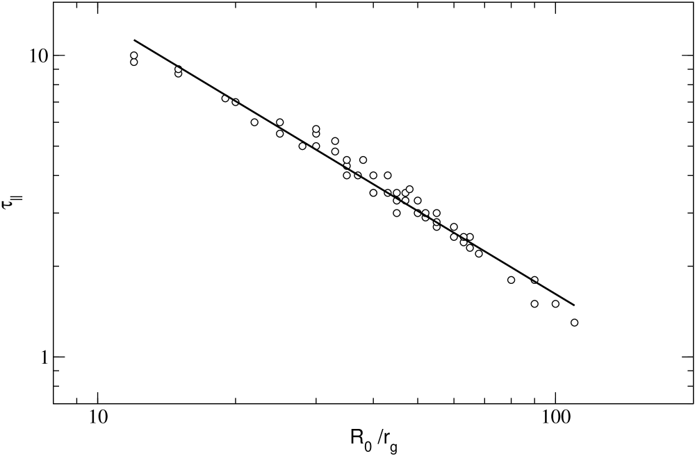
Figure 3: The model $R_{0}$ and ${\tau}_{\parallel}$ values that result in the $\Gamma$ and $<t_{\rm lag}>$ values of Fig. 2, and which agree with the Pottschmidt et al. (2003) results.

However, even more interesting is that, for the model to explain the observational spectral index – time lag relation, $R_{0}$ and $\tau_{\parallel}$ must change in a highly correlated way: as $R_{0}$ increases, $\tau_{\parallel}$ must decrease. In fact, we find that a straight-line fit to the points (Fig. 3) is very close to a $\tau_{\parallel}$ (or $n_{0}$) $\propto R_{0}^{-1}$ relation. Generally speaking, when $R_{0}$ increases, so does the average time lag. The spectrum should also harden at the same time. However, if $\tau_{\parallel}$ (or $n_{0}$) decreases inversely proportional to $R_{0}$, it affects the spectrum more and forces it to steepen exactly as observed.

Pottschmidt et al. (2003) computed $\Gamma$ and $<t_{\rm lag}>$ using data from RXTE observations that lasted $2-7$ ks and were performed every $\sim 10$ days over a period of 3.5 years. In effect, these values characterize the long-term evolution of the physical characteristics of the X-ray emitting source. The results that we present in this work show that our jet model can explain these long-term changes if we assume reasonable variations of just two model parameters, namely the width of the jet at its base and the optical depth along the jet axis.

It is important to point out that the $n_{0}\propto R_{0}^{-1}$ (or $\tau_{\parallel}\propto R_{0}^{-1}$, if all other parameters are kept at their reference values) relation implies (via the continuity equation) that $\dot{M}_{\rm out}(R_{0})\propto R_{0}$, i.e., that the mass ejection rate in the jet increases linearly with $R_{0}$.

3.2 The spectral index – Lorentzian peak frequencies relation

We can also explain, to some extent, the “$\Gamma$–Lorentzian peak frequencies” relation as follows. As mentioned in the Introduction, $M_{\rm out}/\dot{M}_{\rm out}$ is a characteristic timescale for ejecting all the available mass. If the ejection process operates as a damped oscillator with frequency proportional to the inverse of this time scale, i.e., frequency $=C\dot{M}_{\rm out}/M_{\rm out}$ (where $C$ is a proportionality constant), then $n_{0}$ and $R_{0}$, and hence the emitted jet flux, will vary with the same frequency. As a result, a Lorentzian with frequency $C\dot{M}_{\rm out}/M_{\rm out}=C\pi m_{p}v_{\parallel}R_{0}^{2}n_{0}/M_{\rm out}=C^{\prime}R_{0}^{2}n_{0}$ will appear in the power spectrum. Here we have assumed that $M_{\rm out}$ and $v_{\parallel}$ are constant.

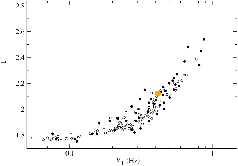
Figure 4: Correlation between the photon number spectral index $\Gamma$ and the frequency $\nu_{1}$ of the first Lorentzian component of the power spectrum. Empty circles are from Pottschmidt et al. (2003) and filled circles are the results of our model. The larger grey circle represents the model with the reference values of the parameters.

In Fig. 4 we plot $\Gamma$ versus $\nu_{1}$, i.e. the peak frequency of the first Lorentzian of Pottschmidt et al. (2003) and the $\Gamma$ versus $C^{\prime}R_{0}^{2}n_{0}$ plot that result from our simulations, using the same $R_{0}$ and $n_{0}$ parameter values, which reproduce the $\Gamma-<t_{\rm lag}>$ relation of Pottschmidt et al. (2003) (i.e., the values plotted in Fig. 3) for $C^{\prime}=1.2\times 10^{-33}$ cm s^-1. Clearly, the model-predicted “$\Gamma$–Lorentzian peak frequency $\nu_{1}$” relation agrees with the data.

Here $C^{\prime}$ is one extra model parameter, whose value is difficult to interpret at the moment (as it should be associated with the unknown details of the ejection mechanism at the base of the jet). This parameter is necessary for adjusting the normalization of the $\Gamma-\nu_{1}$ relation. However, according to our model, the shape of this relation only relies on the dependence on $R_{0}$ and $n_{0}$ through the combination $R_{0}^{2}n_{0}$. We believe that the similarity between the shape of the observed and the model-predicted $\Gamma-\nu_{1}$ relation, when $R_{0}$ and $n_{0}$ take the same values that reproduce the $\Gamma-<t_{\rm lag}>$ relation, is an encouraging result, which supports our model. Since the ratios of the Lorentzian peak frequencies $\nu_{i},i=1,2,3,4,$ in Cyg X-1 are constant, there is no need to reproduce the $\Gamma-\nu_{j},j=2,3,4,$ correlations.

We note that the $\nu_{i}\propto R_{0}^{2}n_{0}$ relation, combined with the $n_{0}\propto R_{0}^{-1}$ one (which is necessary for the model to explain the $\Gamma$ - $<t_{\rm lag}>$ correlation as we showed above), implies that $\nu_{i}\propto R_{0}$. In other words, we can explain the relation between $\Gamma$ and Lorentzian peak frequencies only if these frequencies increase with increasing $R_{0}$. This is contrary to what is usually assumed, i.e., that time scales increase with increasing size, and hence that frequencies should decrease with increasing $R_{0}$.

In our case, the $\nu_{i}\propto R_{0}$ relation is due to the fact that we assumed that $M_{\rm out}$ does not depend on radius. If the mass ejection rate in the jet increases with $R_{0}$ (as the model requires so that $n_{0}\propto R_{0}^{-1}$, and hence $\Gamma$ and $<t_{\rm lag}>$ correlate as observed) then the time scale needed to eject all the available mass to the jet should naturally decrease with increasing radius.

3.3 The $\Gamma$ – radio flux relation

If indeed it is $n_{0}$ and $R_{0}$ that vary with time in such a way that $n_{0}\propto R_{0}^{-1}$, then we expect that the radio flux should also vary, even if all the other model parameters remain constant. In fact, it is reasonable to believe that there will be a correlation between this flux and $\Gamma$, time lags, and Lorentzian frequencies. It is this possibility that we investigate in this section.

The radio emission of the jet in our model is a result of the synchrotron emission of the fast-moving electrons in the magnetic field of the jet. The accurate calculation of the complete synchrotron spectrum can be achieved numerically by dividing the jet in slices across the $z$-axis, and calculating the synchrotron emission and absorption in each slice assuming a power-law electron distribution (Paper III). There it is shown that the radio emission from the jet is characterized by a flat spectrum with flux density close to observations. For the purposes of this work, we derive the scaling of the radio flux density with the model parameters.

The observed flux density $P_{\nu}$ that comes for height $z$ of the jet scales as (e.g. Rybicki & Lightman 1979)

$$P_{\nu}\propto C_{\alpha}B^{\frac{\alpha+1}{2}}\gamma_{\rm min}^{\alpha-1}n_{e}\nu^{\frac{1-\alpha}{2}}R^{2}(z)z,$$

where $\gamma_{min}$ stands for the minimum Lorentz factor of the electron distribution, and $\alpha$ for its power-law exponent (Paper III). The function $C_{\alpha}$ depends only on the index $\alpha$. Using Eqs. (1), (3), and (4), the last expression can be rewritten as

$$P_{\nu}\propto C_{\alpha}B_{0}^{\frac{\alpha+1}{2}}\gamma_{\rm min}^{\alpha-1}n_{0}\nu^{\frac{1-\alpha}{2}}R_{0}^{2}z_{0}(z/z_{0})^{\frac{1-\alpha}{2}}.$$

The synchrotron radiation is strongly self-absorbed below a characteristic frequency (the turn-over frequency) $\nu_{\rm t}$. The synchrotron absorption coefficient is given by the expression (e.g. Rybicki & Lightman 1979)

$$a_{\nu}=A_{\alpha}n_{e}\gamma_{\rm min}^{\alpha-1}B^{\frac{\alpha+2}{2}}\nu^{-\frac{\alpha+4}{2}},$$

where $A_{\alpha}$ only depends on the index $\alpha$. The turn-over frequency in a slice of the jet can be estimated as the frequency for which the optical depth to synchrotron absorption becomes unity across the width of the jet, i.e., $a_{\nu}R(z)\simeq 1$. Solving this expression for $z_{\nu}/z_{0}$ and using Eqs. (1), (3), (4), and (8), we have

$$z_{\nu}/z_{0}=A^{\prime}_{\alpha}\nu^{-\frac{\alpha+4}{\alpha+3}}n_{0}^{\frac{2}{\alpha+3}}\gamma_{\rm min}^{\frac{2\alpha-2}{\alpha+3}}B_{0}^{\frac{\alpha+2}{\alpha+3}}R_{0}^{\frac{2}{\alpha+3}}.$$

Most of the emission seen at frequency $\nu$ comes from the height of the jet that corresponds to the thick-thin transition $z_{\nu}$. Inserting expression (9) into expression (7) and using Eq. (2), we have for the radio flux density, $P_{\nu}$, that one measures at a certain frequency, $\nu$,

$$P_{\nu}\propto C^{\prime}_{\alpha}R_{0}^{\frac{\alpha+7}{\alpha+3}}z_{0}^{\frac{\alpha-1}{\alpha+3}}B_{0}^{\frac{3\alpha+5}{2\alpha+6}}\tau_{\parallel}^{\frac{4}{\alpha+3}}\gamma_{\rm min}^{\frac{4\alpha-4}{\alpha+3}}\nu^{\frac{\alpha-1}{2\alpha+6}},$$

where $C^{\prime}_{\alpha}$ is a decreasing function of $\alpha$. This is expected since a steeper electron distribution (with the rest of the parameters fixed) leads to weaker radio emission.

If only $R_{0}$ and $\tau_{\parallel}$ vary with time according to the relation $\tau_{\parallel}\propto R_{0}^{-1}$ as we argued above, then the above equation implies that $P_{\nu}\propto R_{0}^{\frac{\alpha+7}{\alpha+3}}R_{0}^{\frac{-4}{\alpha+3}}$ or $P_{\nu}\propto R_{0}$. In other words, we expect the radio flux to increase with increasing width of the jet. Since as $R_{0}$ increases (and $n_{0}\propto R_{0}^{-1}$) the spectrum steepens, we should also expect a positive correlation between $P_{\nu}$ and $\Gamma$: the radio flux should increase as the spectrum steepens.

In Fig. 5 we plot the average 15 GHz radio flux, $P_{15\rm GHz}$, as observed with the Ryle telescope, binned over a period of $\pm 2$ days before and after the time of the RXTE observations that Pottschmidt et al. (2003) used to determine $\Gamma$. (The results do not change significantly if we bin the radio light curve using a smaller or a larger bin size.) One can see that there is a general trend for $P_{15\rm GHz}$ to increase with increasing $\Gamma$, as expected, until $\Gamma$ reaches the value of $\sim 2.2$. When we use the $(P_{15\rm GHz},\Gamma<2.2)$ data points to compute Kendall’s $\tau$, we find that $\tau=0.21$. The probability of obtaining this value in the case of no association between $P_{15\rm GHz}$ and $\Gamma$ is less than 0.2%. We conclude that, as long as $\Gamma<2.2$, there is a weak, but statistically significant, correlation between $P_{15\rm GHz}$ and $\Gamma$ in the sense that, on average, the radio flux increases as the spectrum steepens.

According to Eq. (10), the break of the $P_{15\rm GHz}-\Gamma$ correlation at $\Gamma\approx 2.2$, as the source moves into intermediate/transition states (and then to the thermal state), suggests that, as $R_{0}$ keeps increasing, then $B_{0}$ may decrease. Alternatively, the transition may be characterized by weaker particle acceleration leading to either lower values of $\gamma_{\rm min}$ or higher values of the electron index $\alpha$. If real, this result offers a hint as to what happens as the source approaches the thermal state: the width of the jet increases and the magnetic field diminishes (which explains the silence in radio) and there is weaker particle acceleration taking place in the jet (which explains the weaker X-ray power-law emission).

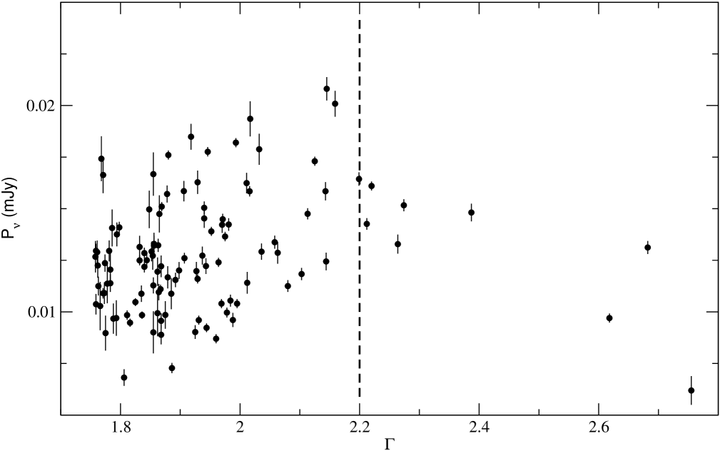
Figure 5: The 15 GHz flux vs the photon number spectral index, $\Gamma$, of Cyg X-1 between 1998 and 2001.

4 Summary and conclusions

In a series of three papers (Papers I, II, and III) it has been shown that our jet model can explain a number of observations regarding black-hole X-ray binaries in the hard state. These are: a) the energy spectrum from radio to hard X-rays; b) the time-lag of the hard photons relative to the softer ones as a function of Fourier frequency; c) the flattening of the power spectra at high frequencies with increasing photon energy and the narrowing of the autocorrelation function.

In this paper we investigate whether our model can explain the long term variations in the spectral and timing properties of Cyg X-1, which are closely linked. The main result of our work is that we can reproduce the $\Gamma-<t_{\rm lag}>$ correlation of Pottschmidt et al. (2003) if we assume reasonable variations in just two model parameters around their mean values: the width of the jet at its base and the optical depth along the jet’s axis (or equivalently the electron density at the base of the jet). We find that, if $\tau_{\parallel}\approx 1.5-10$, $R_{0}\approx 5-50r_{s}$ and $\tau_{\parallel}\propto R_{0}^{-1}$, then the model predicts a $\Gamma-<t_{\rm lag}>$ relation that is almost identical to the one that Pottschmidt et al. (2003) observed. Furthermore, if the flux variability operates on a time scale which is proportional to $M_{\rm out}/\dot{M}_{\rm out}$ (i.e. the characteristic time needed to eject all the available matter to the jet), then the same $\tau$ and $R_{0}$ variations can also explain the shape of the “spectral index - Lorentzian peak frequencies” correlation of Pottschmidt et al. (2003). Finally, given the model parameter variations that are needed to explain the observed ”spectral - timing” correlations, the model predicts a ”radio flux – $\Gamma$” correlation, which, as we show, does indeed hold in Cyg X-1.

The $\tau_{\parallel}\propto R_{0}^{-1}$ relation, which is necessary to explain the observed $\Gamma-<t_{\rm lag}>$ relation, is a natural outcome of the model if simply $\dot{M}_{\rm out}\propto R_{0}$. We propose that this is the underlying “fundamental” relation that governs the long-term evolution of the physical characteristics of the jet, hence of the observational spectral and timing properties of the source. The physical reason for this relation is unclear at the moment; but whatever its origin, the relation itself does make sense because as the rate of the mass ejected in the jet increases, it seems reasonable to assume that the jet will become “bigger”, i.e. $R_{0}$ will also increase. In fact, in this way, one can explain reasonably well all the long-term observed changes with variations in one fundamental physical parameter of the system, namely the accretion rate. As the accretion rate increases, $\dot{M}_{\rm out}$ should also increase. If the jet size increases proportionally to $\dot{M}_{\rm out}$, then $n_{0}\propto R_{0}^{-1}$, and hence the $\Gamma$ – $<t_{\rm lag}>$ relation. We hope that this “accretion rate – ejection rate – jet size” relation will provide an important and useful hint for all models that try to explain the connection between accretion flows and outflows, hence the formation of jets in regions close to the central engines in accreting compact objects.

We find that the $\dot{M}_{\rm out}\propto R_{0}$ relation predicts that the radio flux should increase linearly with the photon number spectral index. To the best of our knowledge, such a relation has never been suggested or even detected either in Cyg X-1 or in any other GBH in the past. We show that a linear “radio flux – spectral index” relation does exist on long time scales in Cyg X-1. We believe that this result strongly supports our view that a) X-rays in Cyg X-1 are produced by Compton upscattering in the jet of soft photons from the accretion disk and b) the jet’s size and optical depth evolve with time because $\dot{M}_{\rm out}\propto R_{0}$. Furthermore, that the “radio flux – spectral index” relation breaks at index values higher than $\sim 2.2$, provides interesting hints into what may be happening as the source moves to the intermediate and thermal state. Most probably the magnetic field decreases and/or there is weaker particle acceleration in the jet (i.e. the electron distribution index, $\alpha$, becomes larger) as the accretion rate increases (as inferred from the increase in the disk thermal emission).

The explanation of the short time-scale variability properties of Cyg X-1 is significantly more challenging. Our model cannot explain why four Lorentzian components exist in the source’s power spectrum (assuming of course that the Lorentzians are the fundamental building blocks of the power spectrum in Cyg X-1 and other GBHs). However, it can explain, to some extent, the way they vary with the source’s photon number spectral index. If indeed the long-term evolution of the source is governed by variations in $R_{0}$ and $\dot{M}_{\rm out}$, it is natural to assume that the short-term variations are caused by short-term, random variations of $\dot{M}_{\rm out}$ (and hence of $n_{0}$ or $\tau_{\parallel}$, and finally X-ray flux), around its mean value. We find that, if these variations operate on a time scale that is proportional to the characteristic time needed to eject all the available matter to the jet, then the model can explain the $\it shape$ of the “$\Gamma$ - Lorentzian peak frequencies” relations of Pottschmidt et al. (2003). There is no reason why the model “$\Gamma-$ inverse time needed to eject the mass to the jet” relation should have the same shape as the observed “$\Gamma-$ Lorentzian peak frequencies”. Thus we do not find this agreement to be coincidental. Instead, it is one more evidence in favor of the jet model and the parameters’ evolution we present in this work, and we find it operates on long time scales in Cyg X-1.

Our results suggest that the characteristic frequencies seen in the power spectrum should increase with increasing size of the source, i.e. $R_{0}$, a result that goes against current views. However, the characteristic frequencies may not scale directly with the source size, but with accretion rate, hence $\dot{M}_{\rm out}$. As argued above, it seems reasonable to think that, as the accretion rate increases, so too the mass ejection rate to the jet. Perhaps, then, it is the accretion rate (through $\dot{M}_{\rm out}$) that drives the variations in both $R_{0}$ and on the characteristic time scales. A physical explanation as to how this may happen and as to the value (and number) of characteristic time scales, requires knowledge of the details of the acceleration/ejection process of the jet, and is beyond the scope of the present work. However, as we mentioned above, we hope that the results we present here will help the investigation of the proper mechanism responsible for the launch of the jets and winds in accreting compact objects.

We note that our conclusion, presented in Sect. 3.2, that the Lorentzian peak frequencies $\nu_{i}$ increase with the size $R_{0}$ of the base of the jet, holds for a given source (in our case Cyg X-1). If one wanted to extend our model to other sources, then the mass of the black hole comes in. The argument goes as follows: Making the reasonable assumption that $M_{\rm out}\propto R_{0}^{2}$ and using $n_{0}\propto R_{0}^{-1}$, we find that the $\nu_{i}$ scale as $1/R_{0}$. Since $R_{0}$ is typically a few times $r_{g}$, we conclude that the Lorentzian peak frequencies $\nu_{i}$ are inversely proportional to the mass of the black hole.

In closing, we want to point out that the above results and conclusions are consistent with the fact that, in the thermal state of Cyg X-1, the time lags versus Fourier frequency are identical to those in the hard state (Pottschmidt et al. 2000). In the thermal state, the radio emission is very weak and possibly undetectable, but we think that the jet is there and that it produces, by Comptonization, both the time lags versus Fourier frequency and the steep power-law energy spectrum above $\sim 10$ keV. According to our model, the suppression of both the radio and the X-ray emission in this state should be caused by a magnetic field suppression and a weaker particle acceleration, respectively.