Degeneracies in the length spectra of metric graphs

Abstract

The spectral theory of quantum graphs is related via an exact trace formula with the spectrum of the lengths of periodic orbits (cycles) on the graphs. The latter is a degenerate spectrum, and understanding its structure (i.e., finding out how many different lengths exist for periodic orbits with a given period and the average number of periodic orbits with the same length) is necessary for the systematic study of spectral fluctuations using the trace formula. This is a combinatorial problem which we solve exactly for complete (fully connected) graphs with arbitrary number of vertices.

1 Introduction

The interest in the spectral properties of the Schrödinger operator on metric graphs (known also as ”quantum graphs”) increased dramatically after it was found that quantum graphs provide an excellent paradigm for the study of spectral fluctuations in quantum chaotic systems [2, 3]: The spectral density of quantum graphs can be expressed as an exact trace formula [1, 2] in terms of the spectrum of the lengths of its periodic orbits (PO) (also called cycles) which is analogous to the asymptotic semi-classical trace formula [4]. Moreover, the quantum graphs posses a Liouvillian analogue, which, under some well understood conditions is ergodic. At the same time, extensive numerical simulations and tests can be performed with rather modest computational effort allowing detailed comparison of the spectral statistics with the prediction of Random Matrix Theory, and study the systematic deviation from it. The simple finite graphs are essentially one dimensional (albeit not simply connected) systems. They display spectral complexity under one important condition: the lengths of the bonds must be rationally independent.

The main tool in the theoretical discussion of the spectral statistics of quantum graphs is the above-mentioned trace formula. It can be written explicitly as

$$d(k)=\sum_{j=1}^{\infty}\delta(k-k_{j})=\frac{\mathcal{L}}{\pi}+\sum_{n}\sum_{p\in\mathcal{P}_{n}}A^{(n)}_{p}{\rm e}^{ikl_{p}}\ ,$$ (1)

where $E_{j}=k_{j}^{2}$ are the eigenvalues of the Schrödinger operator. The $k_{j}$’s form the wave-number spectrum. $\mathcal{L}$ is the total bond length, i.e., for a graph with $B$ bonds, of lengths $L_{b}$, it is given by $\mathcal{L}=\sum_{b=1}^{B}L_{b}$. $\mathcal{P}_{n}$ denotes the set of PO’s of period $n$. Each periodic orbit contributes a term which consists of a ”transition amplitude” $A^{(n)}_{p}$, and a unimodular factor with a phase which is determined by the length of the corresponding $n$-bond PO

$$l_{p}=\sum_{b=1}^{B}q_{b}L_{b}\ \ \ \ ;\ \ \ q_{b}\in\{0,1,2,\cdots\}\ \ {\rm and}\ \ \sum_{b=1}^{B}q_{b}=n\ .$$ (2)

The length spectrum is highly degenerate. Each degeneracy class contains all orbits which traverse the same bonds the same number of times, but not in the same order (up to cyclic permutations) and only these (since the bond lengths $L_{b}$ are rationally independent). That is, a degeneracy class of n-bond PO’s consists of orbits which have the same code ${\bf q}^{(n)}=(q_{1},\cdots,q_{B})$, with $\sum_{b}q_{b}=n$. Not every set of nonnegative integers $\{q_{b}\}$ the sum of which is $n$ represents a degeneracy class - the graph connectivity and the periodicity restrict the possible codes. The trace formula can be written as

$$d(k)=\frac{\mathcal{L}}{\pi}+\sum_{n}\sum_{{\bf q}^{(n)}}\ \left[\sum_{p\in{\bf q}^{(n)}}A^{(n)}_{p}\ \right]{\rm e}^{ikl_{\bf q}^{(n)}}\ ,$$ (3)

Where the contributions of the different orbits in the degeneracy class ${\bf q}^{(n)}$ were lumped together to the sum in the square brackets, all having the same phase factor.

There are two prominent examples where a detailed information about the degeneracy classes is needed. The first example emerges in attempts to understand the conditions under which the spectral fluctuation of a quantum graph follow the predictions of Random Matrix Theory. A standard tool is the computation of the spectral autocorrelation function

$$R(\xi;k)=\frac{1}{2\Delta}\int_{k-\Delta}^{k+\Delta}\tilde{d}(x+\frac{\xi}{2})\tilde{d}(x-\frac{\xi}{2}){\rm d}x\ ,$$ (4)

where $\tilde{d}(k)=d(k)-\frac{\mathcal{L}}{\pi}$ is the fluctuating part of the spectral density and the domain of integration $[k-\Delta,k+\Delta]$ is arbitrarily large. Substituting the explicit expression (3) in (4) one sees that the autocorrelation function depends on the squares of the individual contributions of the degeneracy classes (the terms in square brackets in (3)).

The second example is encountered in the context of ”hearing the shape of a graph”, that is, in attempts to reconstruct the connectivity and the length spectrum from the energy eigenvalue spectrum of the quantum graph [9]. The main tool is again the trace formula (3) or rather its Fourier transform $\hat{d}(l)=\int{\rm d}kd(k)\exp(ikl)$. $\hat{d}(l)$ is a distribution supported on the length spectrum, with weights which can be read off from (3). The length spectrum (its composition and weights) is therefore useful to obtain the information about $\hat{d}(l)$ and in turn also about the connectivity of the graph.

The leading asymptotic (for large $n$) contribution to the number of degeneracy classes in a general connected graph was obtained by Berkolaiko [5]. The number of degeneracy classes and the number of PO’s in each class were obtained by Tanner [6] for binary graphs up to order 6.

In this paper we present an exact expression for the number of classes for fully connected (complete) graphs of any order.

We start by defining precisely graphs, PO’s, and their degeneracy classes. We then compute the number of degeneracy classes for general fully connected graphs, the total number of n-bond PO’s, and obtain the mean degeneracy of the classes as the ratio between the two. Finally, we present numerical results and interpret them.

2 Graphs, Periodic orbits, Degeneracy classes

A graph, $G,$ of order $V,$ is a set of $V$ numbered vertices, some of which are connected by a bond (no more than one bond between two vertices, no bond connects a vertex to itself). The number of bonds connected to a vertex is the vertex valency. The connectivity matrix of $G$ is defined by

$$C_{ij}(G)=\{\begin{array}[]{rr}1&if~{}i~{}and~{}j~{}are~{}connected\\ 0&otherwise.\end{array}$$ (7)

A fully connected simple graph $K_{V}$ is a graph where each vertex is connected by a single bond to any other vertex (beside itself): $C_{i,j}=1-\delta_{i,j},~{}i,j\in G.$

A periodic orbit (PO) on a graph G is a sequence of vertices, $[v_{1},v_{2},...,v_{n}]$ with $C_{v_{i},v_{i+1}}=1$ and $v_{1}=v_{n}.$ PO’s that can be obtained from one another by a cyclic permutation of their vertices will be considered identical.

Consider an integer set $\{q_{b}\}_{b=(i,j)=(j,i)},~{}i,j\in G$ with $\sum q_{b}=n.$ A degeneracy class of $n$-bond periodic orbits is a set of all the n-bond PO’s each of which passes exactly $q_{b}$ times over the bond $b.$ All these PO’s are of the same length and since the bond lengths are rationally independent - all PO’s of the same length belong to one class. The degeneracy of a class is the number of distinct PO’s in it. Fig. 1.a shows the fully connected graph $G=K_{5}.$ Fig. 1.b shows the degeneracy class $(q_{(1,2)}=q_{(2,4)}=q_{(4,5)}=q_{(5,1)}=1,q_{(1,4)}=2).$ Fig. 1.c lists all the PO’s in this class and Fig 1.d shows two of them explicitly.

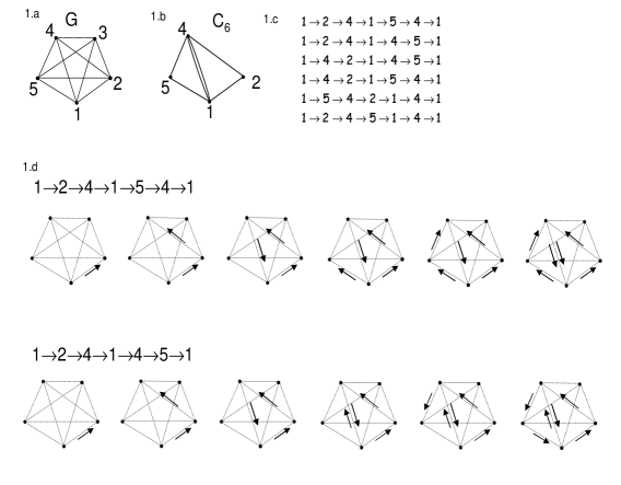
Figure 1: The fully connected graph $K_{5}$ and one of its degeneracy class

Let $N_{c}(n,G)$ be the number of classes of $n$-bond PO’s in $G$ and $N_{p}(n,G)$ the total number of $n$-bond PO’s in $G.$ The mean degeneracy of n-bond PO in $G,$ $D_{n}(G),$ is defined by:

$$D_{n}(G)\equiv\frac{N_{p}(n,G)}{N_{c}(n,G)}.$$ (8)

In the next section we shall provide exact expressions for $N_{c}(n,K_{V}),$ $N_{p}(n,K_{V}),$ and $D_{n}(K_{V}),$ that is, for the number of classes and PO’s, and the mean degeneracy of fully connected simple graphs.

3 The number of classes of $n$-bond periodic orbits on a fully connected graph with $V$ vertices

Since a fully-connected graph is determined uniquely by specifying $V,$ we may use more compact notations, replacing $D_{n}(K_{V})\rightarrow D(n,V)$ and so on. We start by obtaining $N_{c}(n,V).$

Let $v\leq V$ and $N_{c,v}(n,v)$ be the number of $n$-bond degeneracy classes in $K_{v}$ which contain PO’s that passes through all the $v$ vertices. Note that $N_{c,v}(n,v)\leq N_{c}(n,v)$ because not all PO’s pass through all the vertices. More precisely,

$$N_{c}(n,V)=\sum_{v=1}^{V}{V\choose v}N_{c,v}(n,v)$$ (9)

that is, the number of classes is a sum of the number of classes with PO’s that use exactly $v$ vertices. The factor ${V\choose v}$ accounts for the possibilities of choosing these $v$ vertices. All such choices have identical contribution since $K_{V}$ is fully connected.

For example consider $n=V=4.$ Figs.2.a, 2.b and 2.c show all the 4-bond classes of $K_{4}$ grouped according to the sum in Eq.(9). There are ${4\choose 2}=6$ ways for choosing 2 vertices (see Fig.2.a), ${4\choose 3}=4$ for choosing 3 vertices (corresponding to each line in Fig.2.b), ${4\choose 4}=1$ ways for choosing 4 vertices (Fig.2.c). These figures shows that, $N_{c,1}(4,1)=0,$ $N_{c,2}(4,2)=1,$ $N_{c,3}(4,3)=3,$ $N_{c,4}(4,4)=4.$

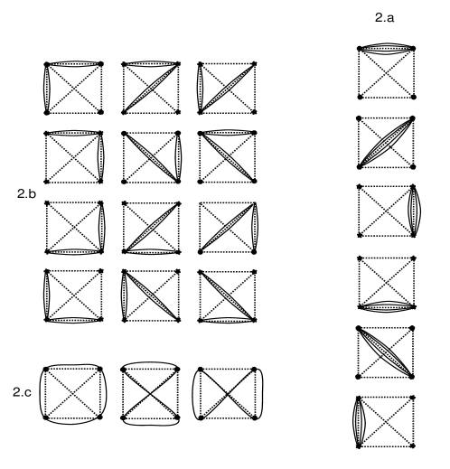
Figure 2: 4-bond degeneracy classes of the fully connected graph $K_{4}$

The reason why we have expressed $N_{c}(n,V)$ in Eq.(9) in terms of $N_{c,v}(n,v)$ is because the latter was calculated by R. C. Read in Ref. [10]. For completeness, a concise derivation along the lines of that work is given in Appendix 1. The result derived in Appendix 1 is that $N_{c,v}(n,v)$ is $v!$ times the coefficient of $x^{v}t^{n}$ in the Taylor expansion (near $t=x=0$) of $\ln\left(E(x,t)\right)$,

$$N_{c,v}(n,v)=\frac{1}{n!}\frac{\partial^{v}}{\partial x^{v}}\frac{\partial^{n}}{\partial t^{n}}\ln\left(E(x,t)\right)|_{x=0,t=0},$$ (10)

where

$$E(x,t)=\sum_{v=0}^{\infty}2^{-v}\frac{x^{v}}{v!}(1-t)^{-\frac{1}{2}v(v-1)}\sum_{s=0}^{v}{v\choose s}\left(\frac{1-t}{1+t}\right)^{s(v-s)}.$$ (11)

From this and Eq.(9) one sees that the number of classes of $n$-bond periodic orbits on a fully connected graph with $V$ vertices is

$$N_{c}(n,V)=\frac{1}{n!}\sum_{v=1}^{V}{V\choose v}\frac{\partial^{v}}{\partial x^{v}}\frac{\partial^{n}}{\partial t^{n}}\ln\left(E(x,t)\right)|_{x=0,t=0}.$$ (12)

An explicit expansion of $E(x,t)$ yields

$$E(x,t)=\sum_{n,v=0..\infty}E_{n,v}t^{n}x^{v}$$ (13)

with

$$E_{n,v}=\sum_{s=0..v}\frac{(-1)^{\mu}}{2^{v}v!}{v\choose s}{\mu+s(v-s)-1\choose\mu}{n-\mu+{s\choose 2}+{v-s\choose 2}-1\choose n-\mu}$$

$$~{}~{}~{}~{}~{}~{}~{}~{}~{}~{}_{\mu=0..n}$$ (14)

One can also derive the following recursion relation (see Appendix 2)

$$N_{c,v}(n,v)=v!E_{n,v}-\sum_{m=0..n}\sum_{k=1..v-1}\frac{(v-1)!}{(k-1)!}N_{c,v}(m,k)E_{n-m,v-k}$$ (15)

which enables a fast numerical calculation of $N_{c}(n,V).$

As an example, consider the case $V=n=4.$ Substituting these values in Eq.(12) one obtains $N_{c}(4,4)=21.$ This result is confirmed in Figs.2.a-c which present all the 21 classes of PO’s. Eq. A.1, in Appendix 1 of Ref. [5] provides the asymptotic behavior, for large $n,$ of the number of classes $N_{c}$ (for any connected graph):

$$N_{c}(2n,V)+N_{c}(2n+1,V)\sim\frac{2^{B-V+1}n^{B-1}}{(B-1)!}(1+O(\frac{1}{n})),$$ (16)

where $B$ is the number of bonds. for the complete-graph one has $B=V(V-1)/2.$ By substituting this value into Eq.(16) we verified numerically that the asymptotic behavior of Eq.(12) for $n\gg V$ matches Eq.(16). The results are shown in Figure 3 which presents the ratio $(N_{c}(n,V)+N_{c}(n+1,V))/(N_{c}^{asymp}(n,V)+N_{c}^{asymp}(n+1,V)),$ for even $n$. The superscript $asympt$ stands for the values obtained using Eq.(16).

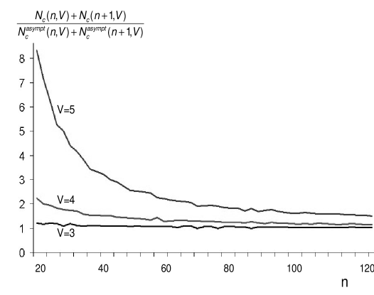
Figure 3: Asymptotic behavior of the number of degeneracy classes

4 The mean degeneracy of $n$-bond periodic orbits on a fully connected graph with $V$ vertices. Numerical results.

To obtain the mean degeneracy Eq. (8), we need also to derive an expression for $N_{p}(n,V)$ i.e. the number of $n$-bond PO’s in $K_{V}.$ Let us first calculate the number of $n$-bond closed trajectories. The number of $n$-bond closed trajectories is given by

$$N(n,V)=TrC^{n}$$ (17)

where $C$ is the connectivity matrix defined in Eq.(7). In our case it is given by:

$$C_{i,j}(K_{V})=1-\delta_{ij},$$ (18)

and its eigenvalues are: $\lambda_{1}=V-1,~{}\lambda_{2}=\lambda_{3}=...\lambda_{V}=-1.$ From Eqs.(17) and (18) it follows that

$$N(n,V)=(V-1)^{n}+(V-1)(-1)^{n}.$$ (19)

$N(n,V)$ is the number of $n$-bond PO’s but is different from $N_{p}(n,V)$ in Eq. (8) since in the latter, PO’s that can be obtained from one another through a cyclic permutation are considered to be the same PO.

For simplicity, let us assume that $n$ is a prime number, thus avoiding the complications arising from the presence of PO’s which are repetitions of a shorter PO. With this assumption, each of the PO’s counted in Eq. (19) is one of $n$ PO’s that can be obtained from one another by cyclic permutations of the vertices. Since we regard all such cyclicly-equivalent PO’s to be the same one, $N_{p}(n,V)$ and $N(n,V)$ are related by

$$N_{p}(n,V)=\frac{1}{n}N(n,V).$$ (20)

From Eqs. (8) and (20) one has

$$D(n,V)=\frac{(n-1)!((V-1)^{n}+(-1)^{n}(V-1))}{\sum_{v=1}^{V}{V\choose v}\frac{\partial^{v}}{\partial x^{v}}\frac{\partial^{n}}{\partial t^{n}}\ln\left(E(x,t)\right)|_{x=0,t=0}}$$ (21)

The mean-degeneracy $D(n,V)$ and its logarithm are shown in Figures 4, 5 and 6. These plots where generated using either Eq.(21) or the recursive relation Eq.(15). Figure 4 presents the $n$-dependence of $D(n,V)$ for fixed values of $V.$ Figure 5 shows the $V$-dependence of $D(n,V)$ for fixed values of $n.$ As seen from these figures, the mean degeneracy grows rapidly and achieves values much larger than 2 already for small (i.e., much smaller than the number of bonds) values of $n.$ On the other hand, in the limit $V/n\rightarrow\infty$ it approaches 2 (most classes contain only a single PO and its time reversal). Approximating $D(n,V)\approx\frac{N(n,V)/n+N(n,V)/(n+1)}{N_{c}(2n,V)+N_{c}(2n+1,V)}$ and then using the asymptotic expression Eq.(16) together with Eq.(19) one has

$$D(n,V)\approx V(V^{2}-V-1)!2^{V-1}\frac{(V-1)^{n}}{n^{V(V-1)/2}}$$ (22)

Taking the logarithm of both sides and keeping only terms containing $n$ (assuming $\log n\ll V$) one obtains

$$\log(D(n,V))\approx n\log(V-1)-\frac{1}{2}V(V-1)\log n.$$ (23)

taking the derivative with respect to $V$ yields the approximate value of $V$ in which the maximal mean-degeneracy is obtained:

$$V_{max}\approx\sqrt{\frac{n}{\log n}}.$$ (24)

Although this estimation was derived for large $n$ it shows reasonable agreement with the peaks in Figure 6. For example, the two maxima marked with arrows, for $n=20$ and $n=30,$ are located in the vicinity of $V=3.9$ and $V=4.5$ respectively, in agreement with Eq.(24).

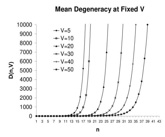
Figure 4: The mean degeneracy for fixed number of vertices, $V.$

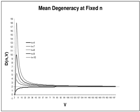
Figure 5: The mean degeneracy at fixed PO’s lengths.

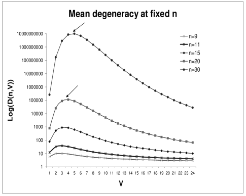
Figure 6: The logarithm of the mean degeneracy at fixed PO’s lengths.

Acknowledgment

We would like to thank G. Berkolaiko for helpful discussions and K. Hornberger for help in the implementation of the Maple code used for producing Fig. 5. This work was supported in part by two Minerva Centers at the Weizmann Institute: The Einstein Center for Theoretical Physics and The Center of Complex Systems, and by the ANR grant number ANR-06-BLAN-0218-01.

Appendix 1. Derivation of Eq. (10)

In this appendix we derive Eq. (10) along the lines of Ref. [10].

Definitions

A graph of order $V$ is a set of $V$ numbered vertices some of which are connected by a bond (no more than one bond between two vertices, no bond connects a vertex to itself i.e. no loops). The number of bonds connected to a vertex is the vertex valency.Fig. 7.1 shows a graph of order 6.

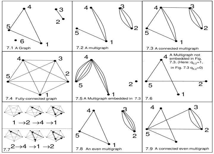
Figure 7: Graphs and Multigraphs

A multigraph is similar to a graph except that there can be more than one bond between two vertices (Fig. 7.2). A graph is a specific case of a multigraph. Let $q_{(i,j)}(g)$ be the number of bonds connecting the vertices $i$ and $j$ in a multigraph $g.$ We shall refer to $q_{(i,j)}(g)$ as the degree of the bond $(i,j)$ in $g.$ For example, in Fig. 7.2 $q_{(2,3)}=q_{(3,2)}=3.$ Note that the pairs (i,j) are not-directed, that is, (i,j) and (j,i) are considered as the same bond.

A multigraph is connected if, by moving on the bonds, one can pass between any two of its vertices (in particular, all valencies are $\geq 1,$ Fig. 7.3). A graph, $K_{V},$ is fully-connected if each of its $V$ vertices is connected to all other vertices (Fig.7.4). Thus, $K_{V}$ has $V(V-1)/2$ bonds.

Let $g$ be a multigraph of order $v.$ $g$ is said to be embedded in a graph $G$ if it can be obtained from $G$ by first adding and deleting bonds between vertices that are connected in $G,$ and then deleting some of the vertices which have zero valency (now, after the addition and deletion of the bonds). By this definition, the order of $G$ is larger or equal to $v.$ If $q_{(i,j)}(G)=1$ then $q_{(i,j)}(g)=0,1,2...$ and if $q_{(i,j)}(G)=0$ then $q_{(i,j)}(g)=0,$. The multigraph in Fig. 7.5 is embedded in the graph of Fig. 7.3 while the multigraph in Fig. 7.6 is not.

A trajectory is a sequence of vertices, adjacent pairs of which are connected. If it is closed, i.e. it starts and ends at the same vertex, the trajectory is a PO. Actually, one can associate several PO’s with each closed trajectory since one can start in any of the trajectory points, however, we shall refer to all of these as a single PO that is say for example that $1\rightarrow 2\rightarrow 4\rightarrow 1$ is the same PO as $2\rightarrow 4\rightarrow 1\rightarrow 2$ and two PO’s are distinct only if they can not be obtained from one another by such a cyclic permutation. Thus, the two closed trajectories in Fig. 7.7 are the same PO.

An even multigraph is a multigraph where each vertex has an even valency (Fig.7.8). For any connected even multigraph (often called Euler multigraph) one can always find a PO that passes on each bond exactly once (Eulerian circuit). Often, there is more than one. For example, the two PO’s (Fig.1.d) $1\rightarrow 2\rightarrow 4\rightarrow 1\rightarrow 5\rightarrow 4\rightarrow 1$ and $1\rightarrow 2\rightarrow 4\rightarrow 1\rightarrow 4\rightarrow 5\rightarrow 1$ passes once on each bond in the connected even multigraph $C_{6}$ shown in Fig. 1.b.

A class of $n$-bond periodic orbits, $C_{n},$ in a graph $G$ is an $n$-bond connected even multigraph which is embedded in a labeled graph $G.$ $C_{n},$ is specified by specifying the set of bond-degrees $\{q_{(i,j)}(C_{n})\}_{i,j\in G},$ where $\sum_{i,j~{}j>i}q_{(i,j)}(C_{n})=n.$ A PO is said to be in $C_{n}$ if it consists of $n$ steps passing exactly $q_{(i,j)}(C_{n})$ times between $i$ and $j.$ By this definition, all PO’s in $C_{n}$ have exactly the same length, independently of the choice of bond lengths and therefore, at a given energy, have the same action. Fig.1.b shows a class of 6-bond PO’s, $C_{6},$ embedded in the fully-connected graph $G$ in Fig.1.a. The PO’s in this class are listed in Fig.1.c. Two of them are drawn in Figs.1.d.

Proof of Eq. (10)

The proof of Eq. (10) is based on that given in Ref. [10] which can also be used to treat the case of classes of graphs with and without loops, and multigraphs with loops. Consider a set of $n$ labeled vertices, and the set $\Omega(n,v)=\{G_{n,v}\}$ of multigraphs with $n$ bonds that one can draw on these $v$ vertices (on means using all of them - i.e. these multigraphs are of order $v$). To each of the $v$ vertices we assign a sign, +1 or -1. There are $2^{v}$ such possible assignments. For a given assignment $S$, we define the sign of each bond in $G_{n,v}$ to be the product of signs of its two vertices. The sign, $\sigma(G_{n,v},S),$ of a multigraph $G_{n,v}\in\Omega(n,v)$ is then defined as the product of signs of all its bonds. Thus,

$$\sigma(G_{n,v},S)=(-1)^{V_{-}(G_{n,v},S)}=(-1)^{\mu(G_{n,v},S)}$$ (25)

where $V_{-}$ is the sum of valencies of the negative vertices and $\mu$ the number of negative bonds. The sum of the signs of $G_{n,v}$ for all possible $S$ is $\sum_{S}(-1)^{V_{-}(G_{n,v})}.$ Summing this over all members of $\Omega(n,v)$ one has

$$\sum_{G_{n,v}\in\Omega(n,v)}\left(\sum_{S}(-1)^{V_{-}(G_{n,v},S)}\right)=\sum_{S}\left(\sum_{G_{n,v}\in\Omega(n,v)}(-1)^{\mu((G_{n,v},S))}\right).$$ (26)

In the right hand side the order of summation was reversed and Eq. (25) was used. Consider the left hand side of Eq. (26). If $G_{n,v}$ is an even multigraph, then $V_{-}(G_{n,v},S)$ is an even number for any $S$ and therefore $\sum_{S}(-1)^{V_{-}(G_{n,v},S)}=2^{v}.$ If $G_{n,v}$ is not even, then at least one of its vertices, say $A,$ has an odd valency. Since for each assignment $S$ in which $A$ is negative there exists $S^{\prime}$ which is identical to $S$ except that $A$ is positive in it, and since $\sigma(G_{n,v},S)=-\sigma(G_{n,v},S^{\prime}),$ one has $\sum_{S}(-1)^{V_{-}(G_{n,v},S)}=0$ for any $G_{n,v}$ which is not even. Thus, the left hand side of Eq. (26) is the number of even multigraphs in $\Omega(n,v)$ times $2^{v}.$ To obtain the right-hand side, consider the ${v\choose s}$ assignments in which exactly $s$ of the vertices are positive. The number of ways to put $\mu$ identical balls in $s(v-s)$ identical boxes each of which may contain any number of balls, is ${\mu+s(v-s)-1\choose\mu}$ and therefore this is the number of ways the $\mu(G_{n,v},S)$ bonds which join the $s$ positive with the $v-s$ negative vertices can be placed. The remaining $n-\mu$ bonds may be placed between the ${s\choose 2}+{v-s\choose 2}$ pairs of vertices with identical signs, that is in

$${n-\mu+{s\choose 2}+{v-s\choose 2}-1\choose n-\mu}$$ (27)

different ways. (To enable compact writing, here and below, we assume that the binomial coefficients have the properties ${a\choose b}=0$ for $b>a$ and $b\neq 0,$ and ${a\choose 0}=1$ for any $a$). Summing over all possible $\mu(G_{n,v},S)$ one gets the total contribution of all assignments in which exactly $s$ vertices are positive:

$$\sum_{\mu=0}^{n}(-1)^{\mu}{\mu+s(v-s)-1\choose\mu}{n-\mu+{s\choose 2}+{v-s\choose 2}-1\choose n-\mu}.$$ (28)

This contribution is the coefficient of $t^{n}$ in $(1-t)^{(-1/2)v(v-1)}(\frac{1-t}{1+t})^{s(v-s)}.$ Thus, the number of $n$-bond even multigraphs one can draw on $v$ labeled vertices is given by $v!$ times the coefficient of $t^{n}x^{v}$ in the power expansion of:

$$E(x,t)=\sum_{v=0}^{\infty}2^{-v}\frac{x^{v}}{v!}(1-t)^{-\frac{1}{2}v(v-1)}\sum_{s=0}^{v}{v\choose s}\left(\frac{1-t}{1+t}\right)^{s(v-s)}.$$ (29)

We are interested in $N_{c,v}(n,v),$ i.e. the number $n$-bond connected even multigraphs one can draw on $v$ labeled vertices. It is a known result in graph enumeration theory that the generating function of the connected set of (labeled) graphs is given by the log of that of the non-connected set [11]. Thus, $N_{c,v}(n,v),$ is $v!$ times the coefficient of $t^{n}x^{v}$ in the power expansion of $\ln(E(x,t))$ which proves Eq.(10).

Appendix 2. Proof of Eq.(15)

Define the expansions

$$E(x,t)=\sum_{v=0}^{\infty}E_{v}(t)x^{v},$$ (30)

and

$$\ln(E(x,t))=\sum_{v=1}^{\infty}L_{v}(t)\frac{x^{v}}{v!}.$$ (31)

$N_{c,v}(n,v)$ is $v!$ times the coefficient of $x^{v}t^{n}$ in $\ln(E(x,t))$ and therefore

$$L_{v}(t)=\sum_{n=0}^{\infty}N_{c,v}(n,v)t^{n}.$$ (32)

There exists a useful recursion relation between the coefficients in Eqs. ( 30) and (31):

$$L_{v}(t)=v!E_{v}(t)-\sum_{k=1}^{v-1}\frac{(v-1)!}{(k-1)!}L_{k}(t)E_{v-k}(t)~{}~{}v>1$$

$$L_{1}(t)=E_{1}(t)~{}~{}~{}$$ (33)

Expansion of Eqs.(31) and (32) in powers of $t$ yields Eq.(15).

References

References

- [1] Jean-Pierre Roth, in: Lectures Notes in Mathematics: Theorie du Potentiel, A. Dold and B. Eckmann, eds. (Springer Verlag) 521-539 (1984).
- [2] T. Kottos and U. Smilansky, Quantum Chaos on Graphs Phys. Rev. Lett. 79,4794- 4797, (1997)
- [3] T. Kottos and U. Smilansky, Periodic orbit theory and spectral statistics for quantum graphs Annals of Physics 274, 76-124 (1999).
- [4] M. G. Gutzwiller, in Chaos in Classical and Quantum Mechanics, Interdisciplinary Applied Mathematics Vol. 1, ed. F. John, (Springer-Verlag, NY), 1990.
- [5] G. Berkolaiko, Quantum Star Graphs and Related Systems, PHD Thesis (Bristol, 2000) unpublished.
- [6] G. Tanner, J. Phys. A 33, 3567-3585 (2001)
- [7] H. Schanz and U. Smilansky, Periodic-Orbit Theory of Anderson-Localization on Graphs, Phys. Rev. Lett. 84 1427-1430 (2000)
- [8] H. Schanz and U. Smilansky, Spectral Statistics for Quantum Graphs : Periodic Orbits and Combinatorics, Philosophical Magazine B80 1999-2021 (2000).
- [9] B. Gutkin and U. Smilansky, Can One Hear the Shape of a Graph?, J. Phys A.31, 6061-6068 (2001).
- [10] R. C. Read, Euler Graphs on Labelled Nodes, Canad. J. Math. 14, 482 (1962).
- [11] F. Harary and E. M. Palmer Graphical Enumeration Ch. 1 Sec. 4 (Academic Press 1973)