Complexity of Quantum States and Reversibility of Quantum Motion

Abstract

We present a quantitative analysis of the reversibility properties of classically chaotic quantum motion. We analyze the connection between reversibility and the rate at which a quantum state acquires a more and more complicated structure in its time evolution. This complexity is characterized by the number ${\cal M}(t)$ of harmonics of the (initially isotropic, i.e. ${\cal M}(0)=0$) Wigner function, which are generated during quantum evolution for the time $t$. We show that, in contrast to the classical exponential increase, this number can grow not faster than linearly and then relate this fact with the degree of reversibility of the quantum motion. To explore the reversibility we reverse the quantum evolution at some moment $T$ immediately after applying at this moment an instant perturbation governed by a strength parameter $\xi$. It follows that there exists a critical perturbation strength, $\xi_{c}\approx\sqrt{2}/{\cal M}(T)$, below which the initial state is well recovered, whereas reversibility disappears when $\xi\gtrsim\xi_{c}(T)$. In the classical limit the number of harmonics proliferates exponentially with time and the motion becomes practically irreversible. The above results are illustrated in the example of the kicked quartic oscillator model.

I Introduction

Strong numerical evidence has been obtained that the quantum evolution is very stable, in sharp contrast to the extreme sensitivity to initial conditions and rapid loss of memory which is the very essence of classical chaos. In computer simulations the latter effect leads to practical irreversibility of classically chaotic dynamics. Indeed, even though the exact equations of motion are reversible, any, however small, imprecision such as computer round-off errors, is magnified by the exponential instability of trajectories to the extent that any memory of the initial conditions is effaced and reversibility is destroyed. In contrast, almost exact reversion is observed in numerical simulations of the quantum motion of classically chaotic systems, even in the regime in which statistical phenomena such as deterministic diffusion take place arrow .

It is intuitive that the physical reasons of this striking difference between quantum and classical motion are rooted in the quantization of the phase space in quantum mechanics. If we consider classical chaotic evolution (governed by the Liouville equation) of some phase space distribution, smaller and smaller scales are explored exponentially fast with time. These fine details of the density distribution are lost due to finite accuracy (inevitable coarse-graining) in numerical simulations, and therefore the reversal of time evolution cannot be carried out. On the other hand, in quantum mechanics one expects that the structure of a quantal phase-space distribution, e.g. of the Wigner function, has resolution limited by the size of the Planck’s cell. While the mean number of Fourier components of the classical phase-space distribution grows exponentially in time for chaotic motion, the number of the components of the Wigner function at any given time is related to the degree of excitation of the system (see for example eq. (69) below) and therefore unrestricted exponential growth of this number is not physical chirikov ; gu ; brumer . This fact implies substantially simpler phase space structure in the case of quantum motion as compared with that of classical chaotic dynamics. We demonstrate below that the mean number of Fourier Harmonics is a simple relevant measure of structural complexity which in turn is related to fundamental properties such as decoherence and entanglement.

In spite of the above arguments, a rigorous link between the intuitively expected different degree of reversibility of quantum and classical motion and the structure developed by the phase-space distributions during dynamical evolution has never been established. The purpose of the present paper is to clarify this problem.

Following the approach developed in ikeda we consider first the forward evolution

$${\hat{\rho}}(t)={\hat{U}(t)}{\hat{\rho}}(0){\hat{U}}^{\dagger}(t)$$ (1)

of an initial (generally mixed) state ${\hat{\rho}}(0)$ up to some time $t=T$. A perturbation ${\hat{P}}(\xi)$ is then applied at this time, with the perturbation strength $\xi$. For our purposes, it will be sufficient to consider unitary perturbations ${\hat{P}}(\xi)=e^{-i\xi{\hat{V}}}$, where ${\hat{V}}$ is a Hermitian operator. The perturbed state

$${\hat{\tilde{\rho}}}(T,\xi)={\hat{P}}(\xi){\hat{\rho}}(T){\hat{P}}^{\dagger}(\xi)$$ (2)

is then evolved backward for the time $T$, thus obtaining the reversed state

$$\begin{array}[]{c}{\hat{\tilde{\rho}}}(0|T,\xi)={\hat{U}}^{{\dagger}}(T){\hat{\tilde{\rho}}}(T,\xi){\hat{U}}(T)=\\ \\ {\hat{P}}(\xi,T){\hat{\rho}}(0){\hat{P}}^{\dagger}(\xi,T),\end{array}$$ (3)

where ${\hat{P}}(\xi,T)\equiv e^{-i\xi{\hat{V}}(T)}$, with ${\hat{V}}(T)\equiv{\hat{U}}^{\dagger}(T){\hat{V}}{\hat{U}}(T)$ being the Heisenberg evolution of the perturbation during the time $T$.

Finally, we investigate the distance between the reversed ${\hat{\tilde{\rho}}}(0|T,\xi)$ and the initial ${\hat{\rho}}(0)$ state, as measured by the Peres fidelity peres

$$\begin{array}[]{c}{\displaystyle F(\xi;T)=\frac{{\rm Tr}[{\hat{\tilde{\rho}}}(0|T,\xi){\hat{\rho}(0)}]}{{\rm Tr}[{\hat{\rho}}^{2}(0)]}}\\ {\displaystyle=\left.\frac{{\rm Tr}[{\hat{\tilde{\rho}}}(t,\xi){\hat{\rho}(t)}]}{{\rm Tr}[{\hat{\rho}}^{2}(t)]}\right|_{t=T}=F\left.(\xi;t)\right|_{t=T}\,.}\end{array}$$ (4)

This quantity is bounded in the interval $[0,1]$ and the distance between the initial and the time-reversed state is small when $F(\xi;T)$ is close to one fidelitynote . In particular, $F(\xi;T)=1$ when the two states coincide. The second line in Eq. (4) is a consequence of the unitary time evolution and will allow us to relate the distance between the initial and the reversed state to the complexity of the state $\hat{\rho}(t)$ at the reversal time $t=T$. This relation will play the key role in our further analysis.

As we have already mentioned above, we characterize the complexity of a quantum state by the structure of its Wigner function. The basic idea here is that a quantum state is complex if this function has a rich phase space structure, which can be naturally measured by the number ${\cal M}(t)$ of its Fourier harmonics. We will show that the fidelity $F(\xi;T)$ is a decreasing function of the complexity ${\cal M}(T)$ of the state ${\hat{\rho}}(T)$. We will prove further that, after the Ehrenfest time scale, namely after a time logarithmically short in the effective Planck constant of the system, the number ${\cal M}(t)$ of harmonics increases notfaster than linearly with time. On the other hand, in classical chaotic dynamics the number of harmonics ${\cal M}_{c}(t)$ of the classical phase-space distribution function grows exponentially in time. We will then ascertain that the initial state is well recovered as long as the perturbation strength $\xi$ is much smaller than a critical perturbation strength $\xi_{c}(T)\sim 1/{\cal M}(T)$. Therefore, $\xi_{c}(T)$ drops exponentially with $T$ in the classical case and not faster than linearly for quantum evolution. This fact explains the much weaker sensitivity of quantum dynamics to perturbations as compared to the classical chaotic motion.

The paper is organized as follows. In Sec. II, we review the main concepts and definitions of quantum mechanics in phase space relevant for our work. In Sec. III, we discuss the kicked quartic oscillator model, used in the remaining part of the paper as a test bed to illustrate the stability properties of classically chaotic quantum motion. In Sec IV, the evolution in time of the harmonics of the Wigner function is studied in detail. In particular, the complexity of the quantum state ${\hat{\rho}}(t)$ is quantified by looking at the sensitivity of the system to an infinitesimal perturbation. In Sec. V, the degree of reversibility of quantum motion, as measured by the Peres fidelity, is related to the number of harmonics developed by dynamics at the reversal time $t=T$. A more detailed study of the reversibility properties of motion is carried out in Sec. VI, where we investigate the properties of the time-reversed state by studying the harmonics of its Wigner function. Finally, the main results of our paper are summarized in Sec. VI.

II Quantum dynamics in the phase space

The phase-space representation of quantum mechanics is a very enlightening approach which allows a direct comparison with classical mechanics gu ; brumer . In this section, we briefly review the main aspects of the phase-space approach which are relevant for our work.

II.1 The Wigner Function

Let us consider a nonlinear system whose dynamics is governed by the Hamiltonian operator ${\hat{H}}\equiv H({\hat{a}}^{{\dagger}},{\hat{a}};t)=H^{(0)}({\hat{n}}={\hat{a}}^{{\dagger}}{\hat{a}})+H^{(1)}({\hat{a}}^{{\dagger}},{\hat{a}};t)$ with the time-independent unperturbed part ${\hat{H}}^{(0)}$ which has a discrete energy spectrum bounded from below so that we can assume that all its eigenvalues $E_{n}^{(0)}\geqslant 0$. Here ${\hat{a}}^{{\dagger}},{\hat{a}}$ are the bosonic, $[{\hat{a}},{\hat{a}}^{{\dagger}}]=1\,$, creation-annihilation operators. We will use the method of c-number $\alpha$-phase space borrowed from the quantum optics (see for example Glauber63 ; Agarwal70 ). This method is equally suitable for analyzing both the quantum and classical evolutions. It is, basically, built upon the basis of the coherent states $|\alpha\rangle$. The latter are defined by the eigenvalue problem ${\hat{a}}|\alpha\rangle=\frac{\alpha}{\sqrt{\hbar}}|\alpha\rangle$, where $\alpha$ is a complex variable independent of $\hbar$. An arbitrary coherent state is obtained from the ground state, $|\alpha\rangle={\hat{D}}\left(\frac{\alpha}{\sqrt{\hbar}}\right)|0\rangle$, with the help of the unitary displacement operator ${\hat{D}}\left(\lambda\right)=\exp(\lambda\,{\hat{a}}^{{\dagger}}-\lambda^{*}{\hat{a}})$.

Using the displacement operator ${\hat{D}}$ as a kernel, one can represent any operator function ${\hat{G}}(t)\equiv G({\hat{a}}^{{\dagger}},{\hat{a}};t)$ in the form of the operator Fourier transformation Agarwal70

$$G({\hat{a}}^{{\dagger}},{\hat{a}};t)=\frac{1}{\pi}\int d^{2}\eta\,{\tilde{G}}(\eta^{*},\eta;t)\,{\hat{D}}(\eta)\,,$$ (5)

where ${\tilde{G}}(\eta^{*},\eta;t)$ is a numerical function of two independent complex variables $\eta^{*},\eta$ and the integration runs over the complex $\eta$-plane. The inverse transformation

$$\tilde{G}(\eta^{*},\eta;t)=Tr\left[G(\hat{a}^{{\dagger}},\hat{a};t)\,\hat{D}^{{\dagger}}(\eta)\right]$$ (6)

is immediately obtained with the help of the orthogonality condition for the displacement operators,

$$\frac{1}{\pi}\,Tr\left[\hat{D}^{{\dagger}}(\eta^{\prime})\,\hat{D}(\eta)\right]=\delta^{(2)}(\eta^{\prime}-\eta)\,.$$ (7)

By using transformation (5), the standard quantum-mechanical formula $\langle Q\rangle=Tr\left[{\hat{\rho}}(t)\,{\hat{Q}}\right]$ for the mean expectation value $\langle Q\rangle$ of a dynamical variable $Q$ [$Q$ is represented by the operator ${\hat{Q}}=Q(\hat{a}^{{\dagger}},\hat{a})$] in a generally mixed state ${\hat{\rho}}(t)=\rho({\hat{a}}^{{\dagger}},{\hat{a}};t)$ can be written in a way formally equivalent to the classical phase space average:

$$\begin{array}[]{c}\langle Q\rangle=\frac{1}{\pi}\int d^{2}\eta\,{\tilde{\rho}}(\eta^{*},\eta;t)\,{\tilde{Q}}(-\eta^{*},-\eta)=\\ \\ \int d^{2}\alpha W(\alpha^{*},\alpha;t)\,Q(\alpha^{*},\alpha)\,.\end{array}$$ (8)

The final form is readily obtained after defining the Wigner function $W(\alpha^{\star},\alpha;t)$ and $Q(\alpha^{\star},\alpha)$ as c-number Fourier transformations of $\tilde{\rho}(\eta^{\star},\eta;t)$ and $\tilde{Q}(\eta^{\star},\eta)$, respectively. The Wigner function in the $\alpha$-phase plane is connected to the density operator $\hat{\rho}(t)$ as

$$\begin{array}[]{c}W(\alpha^{*},\alpha;t)=\frac{1}{\pi^{2}\hbar}\int d^{2}\eta\,\exp\left(\eta\frac{\alpha^{\star}}{\sqrt{\hbar}}-\eta^{\star}\frac{\alpha}{\sqrt{\hbar}}\right)\tilde{\rho}(\eta^{\star},\eta;t)=\\ \frac{1}{\pi^{2}\hbar}\int d^{2}\eta\,\exp\left(\eta^{*}\frac{\alpha}{\sqrt{\hbar}}-\eta\frac{\alpha^{*}}{\sqrt{\hbar}}\right)Tr\left[{\hat{\rho}(t)}\,{\hat{D}(\eta)}\right]\end{array}$$ (9)

(this corresponds to the Weyl’s ordering of the creation-annihilation operators). Similarly,

$$\begin{array}[]{c}Q(\alpha^{*},\alpha)=\frac{1}{\pi}\int d^{2}\eta\,\exp\left(\eta\frac{\alpha^{\star}}{\sqrt{\hbar}}-\eta^{\star}\frac{\alpha}{\sqrt{\hbar}}\right)\tilde{Q}(\eta^{\star},\eta)=\\ \frac{1}{\pi}\int d^{2}\eta\,\exp\left(\eta^{*}\frac{\alpha}{\sqrt{\hbar}}-\eta\frac{\alpha^{*}}{\sqrt{\hbar}}\right)Tr\left[{\hat{Q}}\,{\hat{D}(\eta)}\right]\,.\\ \end{array}$$ (10)

It follows from the definition (9) that the Wigner function is normalized to unity:

$$\int d^{2}\alpha W(\alpha^{*},\alpha;t)=Tr{\hat{\rho}(t)}=1\,.$$ (11)

The Wigner function is real but, unlike its classical counterpart, is not in general positive definite.

With the help of the Wigner function the Peres fidelity (4) can be expressed as

$$\begin{array}[]{c}{\displaystyle F(\xi;T)=\frac{\int d^{2}\alpha\,W\left(\alpha^{*},\alpha;0\right)\tilde{W}\left(\alpha^{*},\alpha;0\big{|}T,\xi\right)}{\int d^{2}\alpha\,W^{2}\left(\alpha^{*},\alpha;0\right)}=}\\ {\displaystyle\frac{\int d^{2}\alpha\,W\left(\alpha^{*},\alpha;T\right)\tilde{W}\left(\alpha^{*},\alpha;T,\xi\right)}{\int d^{2}\alpha\,W^{2}\left(\alpha^{*},\alpha;T\right)}\,.}\end{array}$$ (12)

The important advantage of this representation is that it remains valid in the classical case when the Wigner function reduces to the classical distribution function, $W^{(c)}(\alpha^{*},\alpha;t)\,$.

II.2 Harmonics of the Wigner Function

We define the harmonic’s amplitudes $W_{m}(I;t)$ of the Wigner function by the Fourier expansion

$$W(\alpha^{*},\alpha;t)=\frac{1}{\pi}\,\sum_{m=-\infty}^{\infty}W_{m}(I;t)\,e^{im\theta}\,,$$ (13)

where $\alpha=\sqrt{I}\,e^{-i\theta}\,.$ Then the normalization condition simply implies that $\int_{0}^{\infty}dI\,W_{0}(I;t)=1\,.$ There are no restrictions on $W_{m}$ when $m\neq 0$.

The amplitudes $W_{m}$ can be expressed in terms of the matrix elements $\langle n+m|\hat{\rho}|n\rangle$ along $m$-th subdiagonal of the density matrix. Indeed, using the well-known Schwinger53 matrix elements of the displacement operator in the basis of the eigenvectors $|n\rangle$ of the unperturbed Hamiltonian ${\hat{H}}^{(0)}$,

$$\langle n+m|{\hat{D}}(\eta)|n\rangle={\sqrt{\frac{n!}{(n+m)!}}}\,\eta^{m}\,e^{-\frac{1}{2}|\eta|^{2}}L_{n}^{m}(|\eta|^{2})\,,$$ (14)

($n,m\geq 0$) where $L_{n}^{m}(x)$ is the Laguerre polynomial, the $\eta$-integration in the second line of Eq. (9) can be carried out explicitly. We obtain finally

$$\begin{array}[]{c}W_{m}(I;t)=\frac{2}{\hbar}\,e^{-\frac{2}{\hbar}I}\sum_{n=0}^{\infty}(-1)^{n}\sqrt{\frac{n!}{(n+m)!}}\times\\ \left(4I/\hbar\right)^{\frac{m}{2}}L_{n}^{m}\left(4I/\hbar\right)\langle n+m|{\hat{\rho}}(t)|n\rangle\end{array}$$ (15)

when $m\geq 0$ and $W_{-m}=W_{m\geq 0}^{\star}$.

With the help of the orthogonality condition for the Laguerre polynomials Eq. (15) can be inverted, thus obtaining

$$\begin{array}[]{c}\langle n+m\big{|}{\hat{\rho}}(t)\big{|}n\rangle=(-1)^{n}\,2\sqrt{\frac{n!}{(n+m)!}}\times\\ \int_{0}^{\infty}\!dI\,e^{-2\frac{I}{\hbar}}\,\left(4I/\hbar\right)^{\frac{m}{2}}L_{n}^{m}\left(4I/\hbar\right)\,W_{m}\left(I;t\right)\,.\end{array}$$ (16)

II.3 Time - Evolution of the Wigner Function

The Wigner function satisfies the evolution equation

$$i\frac{\partial}{\partial t}\,W(\alpha^{*},\alpha;t)={\cal\hat{L}}_{q}\,W(\alpha^{*},\alpha;t).$$ (17)

Here ${\cal\hat{L}}_{q}is$ the Hermitian “quantum Liouville operator” ${\cal\hat{L}}_{q}$ whose explicit form is obtained by mapping the standard equation

$$i\frac{\partial}{\partial t}{\hat{\rho}}(t)=\frac{1}{\hbar}[{\hat{H}},{\hat{\rho}}(t)]$$ (18)

onto the $\alpha$-phase space. Supposing that the Hamiltonian can be presented as a Hermitian sum (finite or infinite) of products of the creation-annihilation operators and using then the definitions of the phase space images, Eqs. (9), (10), it is possible to show that (see Ref. Agarwal70 )

$$\begin{array}[]{c}{\cal\hat{L}}_{q}=\frac{1}{\hbar}\left[{\cal H}\left(\alpha^{*}-\frac{\hbar}{2}\frac{\vec{\partial}}{\partial\alpha},\alpha+\frac{\hbar}{2}\frac{\vec{\partial}}{\partial\alpha^{*}}\right)-\right.\\ \left.{\cal H}\left(\alpha^{*}+\frac{\hbar}{2}\frac{\vec{\partial}}{\partial\alpha},\alpha-\frac{\hbar}{2}\frac{\vec{\partial}}{\partial\alpha^{*}}\right)\right],\end{array}$$ (19)

where ${\cal H}(\alpha^{*},\alpha)$ is the phase-space image of the system’s Hamiltonian. The arrows above the derivatives mean that they act only on the arguments of the Wigner function but ignore the $(\alpha^{*},\alpha)$-dependence of the phase-space operator ${\cal H}$ itself. In the classical limit $\hbar=0$ the operator ${\cal\hat{L}}_{q}$ has the standard classical form

$$\hat{{\cal L}}_{c}=\frac{\partial H_{c}(\alpha^{*},\alpha;t)}{\partial\alpha}\,\frac{\partial}{\partial\alpha^{*}}-\frac{\partial H_{c}(\alpha^{*},\alpha;t)}{\partial\alpha^{*}}\,\frac{\partial}{\partial\alpha},$$ (20)

where the classical Hamiltonian function coincides with the diagonal matrix element, $H_{c}(\alpha^{*},\alpha;t)=\langle\alpha|{\hat{H}}^{(N)}({\hat{a}}^{{\dagger}},{\hat{a}})|\alpha\rangle$ of the normal form ${\hat{H}}^{(N)}$ of the quantum Hamiltonian operator. In other words, this function is obtained from the quantum Hamiltonian by substituting ${\hat{a}}\rightarrow\alpha/\sqrt{\hbar}\,,\,\,{\hat{a}}^{{\dagger}}\rightarrow\alpha^{*}/\sqrt{\hbar}\,.$

The outlined phase-space approach is quite general and can be readily extended Glauber63 ; Agarwal70 to systems with arbitrary number of degrees of freedom and is applicable to any system whose Hamiltonian can be expressed in terms of a set of the bosonic creation-annihilation operators . In this approach, the classical distribution function as well as its quantum counterpart are described in terms of the same phase-space variables, thus allowing a straightforward comparison of the two dynamics gu ; brumer .

III The Model

In order to discuss the reversibility/complexity properties of quantum motion, we consider, as an illustrative example, the kicked quartic oscillator model, described by the Hamiltonian Berman78 ; chirikov ; Sokolov84

$${\hat{H}}=H({\hat{a}}^{{\dagger}},{\hat{a}})=\hbar\,\omega_{0}{\hat{n}}+\hbar^{2}\,{\hat{n}}^{2}-\sqrt{\hbar}\,g(t)({\hat{a}}+{\hat{a}}^{{\dagger}}),$$ (21)

where $g(t)=g_{0}\sum_{s}\delta(t-s)$, and ${\hat{n}}={\hat{a}}^{{\dagger}}{\hat{a}}$, $[{\hat{a}},{\hat{a}}^{{\dagger}}]=1$. In our units, the time and parameters $\hbar,\omega_{0}$ as well as the strength of the driving force are dimensionless. The period of the driving force $g(t)$ is set to one. The corresponding classical Hamiltonian function $H_{c}$ can be expressed in terms of complex canonical variables $\alpha,i{\alpha}^{*}$ which are related to the classical action-angle variables $I,\theta$ via $\alpha=\sqrt{I}e^{-i\theta},\alpha^{*}=\sqrt{I}e^{i\theta}$. It reads

$$H_{c}=\omega_{0}|\alpha|^{2}+|\alpha|^{4}-g(t)(\alpha^{*}+\alpha)\,.$$ (22)

Detailed analytical semiclassical analysis of the quantum motion of the model (21) has been presented in Sokolov84 ; Sokolov07 .

The quantum Liouville operator for the model (21) can be derived from Eq. (19) and reads

$$\begin{array}[]{c}{\displaystyle{\cal\hat{L}}_{q}={\cal\hat{L}}_{q}^{(0)}+{\cal\hat{L}}^{(kick)}},\\ \displaystyle{{\cal\hat{L}}_{q}^{(0)}=\left(\omega_{0}-\hbar-\frac{1}{2}\hbar^{2}\frac{\partial^{2}}{\partial\alpha^{*}\partial\alpha}+2|\alpha|^{2}\right)\left(\alpha^{*}\frac{\partial}{\partial\alpha^{*}}-\alpha\frac{\partial}{\partial\alpha}\right)},\\ {\displaystyle{\cal\hat{L}}^{(kick)}=-g(t)\left(\frac{\partial}{\partial\alpha^{*}}-\frac{\partial}{\partial\alpha}\right)}.\end{array}$$ (23)

The essential difference between this operator and the corresponding classical Liouville operator ${\cal\hat{L}}_{c}$ is the presence in Eq. (23) of a term proportional to $\hbar^{2}$ which contains a second derivative over the phase space variables. This term drastically changes the spectrum of the unperturbed part ${\cal\hat{L}}_{q}^{(0)}$ of the Liouville operator and thereby modifies the evolution of the Wigner distribution function $W$ with respect to the classical distribution function $W^{c}$. Indeed, while in the classical limit $\hbar=0$ the factor $\omega_{0}+2|\alpha|^{2}=\omega_{0}+2I=\omega_{c}(I)$ is the continuous frequency of the classical quartic oscillator, the quantum operator ${\hat{K}}\equiv-\frac{1}{2}\hbar^{2}\frac{\partial^{2}}{\partial\alpha^{*}\partial\alpha}+2|\alpha|^{2}$ has a discrete spectrum: considering the real and imaginary parts $(\alpha_{1},\alpha_{2})$ of the variable $\alpha$ as cartesian coordinates, we obtain

$${\hat{K}}=-\frac{\hbar^{2}}{8}\left(\frac{\partial^{2}}{\partial\alpha_{1}^{2}}+\frac{\partial^{2}}{\partial\alpha_{2}^{2}}\right)+2(\alpha_{1}^{2}+\alpha_{2}^{2}).$$ (24)

Therefore, the operator $\hat{K}$ is formally equivalent to the Hamiltonian operator of a two-dimensional isotropic oscillator, with the frequency $\nu=1$ and the mass $\mu=4$. After introducing the standard annihilation-creation operators

$$\begin{array}[]{c}{\hat{A}}_{1,2}=\sqrt{\frac{2}{\hbar}}\,\alpha_{1,2}+\frac{1}{\sqrt{8\hbar}}\,\frac{\partial}{\partial\alpha_{1,2}},\\ {\hat{A}}_{1,2}^{{\dagger}}=\sqrt{\frac{2}{\hbar}}\,\alpha_{1,2}-\frac{1}{\sqrt{8\hbar}}\,\frac{\partial}{\partial\alpha_{1,2}},\end{array}$$ (25)

this operator transforms into ${\hat{K}}=\hbar{\hat{N}}$, where ${\hat{N}}={\hat{N}}_{1}+{\hat{N}}_{2}={A}_{1}^{{\dagger}}{{\hat{A}}_{1}}+{A}_{2}^{{\dagger}}{{\hat{A}}_{2}}$ is the operator representing the total number of fictitious quanta linearly polarized in the $\alpha$-plane. The operator

$$\hat{M}\equiv\left(\alpha^{*}\frac{\partial}{\partial\alpha^{*}}-\alpha\frac{\partial}{\partial\alpha}\right)=-i\frac{\partial}{\partial\theta}$$ (26)

is proportional to the angular momentum projection operator along the axis orthogonal to the $\alpha$-plane and has the discrete eigenvalue spectrum $m=0,\pm 1,\pm 2,...$. We can therefore conclude that the spectrum of the operator

$${\cal\hat{L}}_{q}^{(0)}=\left(\omega_{0}+\hbar\,{\hat{N}}\right){\hat{M}}$$ (27)

is also discrete with eigenvalues $(\lambda_{0})_{n,m}=(\omega_{0}+\hbar n)m$. Since the operators ${\hat{N}}$ and ${\hat{M}}$ commute, operator (27) is Hermitian.

The two linearly polarized quanta introduced above are coupled to each other because the angular momentum operator $\hbar{\hat{M}}=\frac{1}{i}\left({\hat{A}}_{1}^{{\dagger}}{\hat{A}}_{2}-{\hat{A}}_{2}^{{\dagger}}{\hat{A}}_{1}\right)$ is not diagonal in the chosen representation. However both the operators $\hbar{\hat{N}}$ and $\hbar{\hat{M}}$ are simultaneously diagonalized after introducing the operators

$${\hat{A}}_{+}=\frac{1}{\sqrt{\hbar}}\,\alpha+\frac{\sqrt{\hbar}}{2}\frac{\partial}{\partial\alpha^{*}}\,,\quad{\hat{A}}_{-}=\frac{1}{\sqrt{\hbar}}\,\alpha^{*}+\frac{\sqrt{\hbar}}{2}\frac{\partial}{\partial\alpha}\,,$$ (28)

which describe the circularly polarized quanta. In the new representation

$${\hat{N}}={\hat{N}}_{+}+{\hat{N}}_{-},\,\,\,{\hat{M}}=({\hat{N}}_{+}-{\hat{N}}_{-}),$$ (29)

where ${\hat{N}}_{\pm}={\hat{A}}_{\pm}^{{\dagger}}\,{\hat{A}}_{\pm}$ are the operators representing the numbers $n_{\pm}$ of circularly polarized quanta. These new quanta are decoupled:

$$\begin{array}[]{c}{\cal\hat{L}}_{q}^{(0)}=\left(\omega_{0}+\hbar\,{\hat{N}}\right){\hat{M}}={({\cal\hat{L}}_{0})}_{+}-{({\cal\hat{L}}_{0})}_{-},\\ {({\cal\hat{L}}_{0})}_{\pm}=\omega_{0}\,{\hat{N}}_{\pm}+\hbar{\hat{N}}_{\pm}^{2}\,.\end{array}$$ (30)

The eigenvalues $(\lambda_{0})_{n_{+},n_{-}}=\frac{E^{(0)}_{n_{+}}-E^{(0)}_{n_{-}}}{\hbar}$ of the operator (30) are determined by the distances between the unperturbed energy levels $E_{n_{\pm}}^{(0)}=\hbar\omega_{0}\,n_{\pm}+\hbar^{2}\,n_{\pm}^{2}$ corresponding to the excitation numbers $n_{\pm}=0,1,2,...$. The representation (30) is the most convenient for numerical simulations.

The driving perturbation also decouples in the chosen representation:

$$\begin{array}[]{c}{\cal\hat{L}}^{(kick)}={\cal\hat{L}}_{+}^{(kick)}-{\cal\hat{L}}_{-}^{(kick)}\,,\\ {\cal\hat{L}}_{\pm}^{(kick)}=-g(t)\frac{1}{\sqrt{\hbar}}\left({\hat{A}}_{\pm}+{\hat{A}}_{\pm}^{{\dagger}}\right)\,.\end{array}$$ (31)

It then immediately follows that the one-period unitary evolution operator ${\cal\hat{F}}$ for the Wigner function gets factorized as

$$\begin{array}[]{c}{\cal\hat{F}}={\cal\hat{F}}_{+}\,{\cal\hat{F}}_{-}^{{\dagger}}\,,\quad{\cal\hat{F}}_{\pm}=e^{-i{({\cal\hat{L}}_{0})}_{\pm}}\,{\hat{D}}_{\pm}\left(i\frac{g_{0}}{\sqrt{\hbar}}\right)\,,\\ {\hat{D}}_{\pm}\left(i\frac{g_{0}}{\sqrt{\hbar}}\right)=\exp\left(i\frac{g_{0}}{\sqrt{\hbar}}\left({\hat{A}}_{\pm}+{\hat{A}}_{\pm}^{{\dagger}}\right)\right)\,.\end{array}$$ (32)

The complete set of the eigenvectors $|n_{+}\,n_{-}\rangle=|n_{+}\rangle|n_{-}\rangle$ of the unperturbed operator ${\cal\hat{L}}_{q}^{(0)}$ constitutes the excitation number reference basis for the density matrix,

$$\begin{array}[]{c}{\hat{\rho}(t)}=\sum_{n_{+},n_{-}}|n_{+}\rangle\rho(n_{+},n_{-};t)\langle n_{-}|\,;\\ \rho(n_{+},n_{-};t)=\langle n_{+}|{\hat{\rho}(t)}|n_{-}\rangle\,.\end{array}$$ (33)

The evolution from time $t$ to time $t+1$ reads

$$\begin{array}[]{c}\rho(n_{+},n_{-};t+1)=\langle n_{+}|{\hat{U}}_{1}{\hat{\rho}(t)}{\hat{U}}_{1}^{{\dagger}}|n_{-}\rangle=\\ \sum_{n_{+}^{\prime},n_{-}^{\prime}}\langle n_{+}|{\cal\hat{F}}_{+}|n_{+}^{\prime}\rangle\rho(n_{+}^{\prime},n_{-}^{\prime};t)\langle n_{-}^{\prime}|{\cal\hat{F}}_{-}|n_{-}\rangle^{*}\,.\end{array}$$ (34)

Here

$$\begin{array}[]{c}{\hat{U}}_{1}\equiv{\hat{U}}(t=1)=e^{-\frac{i}{\hbar}{\hat{H}}^{(0)}}\,{\hat{D}}\left(i\frac{g_{0}}{\sqrt{\hbar}}\right)\\ =e^{-i\left(\omega_{0}{\hat{n}}+\hbar{\hat{n}}^{2}\right)}\,e^{i\frac{g_{0}}{\sqrt{\hbar}}\left({\hat{a}}+{\hat{a}}^{{\dagger}}\right)}\end{array}$$ (35)

is the (Floquet) operator for our model, namely the one-period unitary evolution induced by the Hamiltonian (21).

Our numerical simulations are based on the combined application of Eqs. (4), (9), and (34). We calculate numerically the truncated Floquet matrix ${\hat{F}}_{nn^{\prime}}$ in the excitation number representation. Two different strategies have been used.

The first approach is based on Eq. (14), which relates matrix elements of the kick operator ${\hat{D}}\left(i\frac{g_{0}}{\sqrt{\hbar}}\right)$ to the Laguerre polynomials. The free rotation operator $e^{-\frac{i}{\hbar}{\hat{H}}^{(0)}}$ is diagonal and its calculation is trivial. Then the product of the matrices $e^{-\frac{i}{\hbar}{\hat{H}}^{(0)}}$ and $\hat{D}$ is truncated to a square matrix of a finite size $N$. The main disadvantage of this approach is the violation of unitarity of the Floquet operator: its norm is not conserved when the size of a quantum state becomes of the order or larger than $N$.

The second approach is based on the truncation of the Hermitian matrix ${\hat{X}}_{nn^{\prime}}=\langle n|\frac{g_{0}}{\sqrt{\hbar}}\left({\hat{a}}+{\hat{a}}^{{\dagger}}\right)|n^{\prime}\rangle$. Then we numerically diagonalize this matrix, ${\hat{X}}={\hat{v}}{\hat{X}}_{d}{\hat{v}}^{{\dagger}}$, with the aid of a unitary matrix ${\hat{v}}$. In such a way we obtain the truncated kick matrix ${\hat{D}}(i\frac{g_{0}}{\sqrt{\hbar}})={\hat{v}}\exp(i{\hat{X}}_{d}){\hat{v}}^{{\dagger}}$ in the excitation number basis. Multiplying it by the, diagonal in this basis, free rotation matrix $\exp\left(-\frac{i}{\hbar}{\hat{H}}^{(0)}\right)$ (truncated to the same size $N$) and finally diagonalizing the obtained unitary matrix, we arrive at a truncated approximation ${\hat{F}}={\hat{V}}{\hat{F}}_{d}{\hat{V}}^{{\dagger}}$ of the Floquet operator (35) in the excitation number representation. The price paid is the artificial boundary condition at $n=N$ which influences the evolution when the size of a quantum state becomes close to that of the truncated Floquet operator. Even though the final diagonalization problem is, by itself, rather time-consuming the great advantage of this approach is that the computation time does not depend on the considered duration of the evolution. This is due to the fact that $\hat{U}(t)=\hat{F}^{t}={\hat{V}}{\hat{F}}_{d}^{t}{\hat{V}}^{{\dagger}}$ and therefore, independently of $t$, it is sufficient to multiply $3$ matrices to construct $\hat{U}(t)$.

IV Harmonics Dynamics

In this section, we study the time evolution of the harmonics of the Wigner function for the kicked quartic oscillator model. The Wigner function of the initial state is taken to be isotropic, so that only the zero angular harmonic $W_{0}$ of the Wigner function is different from zero. In the course of dynamical evolution the Wigner function becomes more and more structured and this reflects in the excitation of a growing number of harmonics. The complexity of the Wigner function at time $t$ is measured by its sensitivity to an infinitesimal perturbation.

IV.1 Initial Condition

We choose the initial state to be an isotropic mixture of coherent states:

$${\hat{\rho}}(0)=\int d^{2}\overset{\circ}{\alpha}\,{\cal P}(|\overset{\circ}{\alpha}|^{2})|\overset{\circ}{\alpha}\rangle\langle\overset{\circ}{\alpha}|=\sum_{n=0}^{\infty}\,{\rho}_{n}\,|n\rangle\langle n|,$$ (36)

where

$${\rho}_{n}=\frac{\pi}{n!}\int_{0}^{\infty}d\overset{\circ}{I}\,{\cal P}(\overset{\circ}{I})\,e^{-\overset{\circ}{I}/\hbar}\left(\overset{\circ}{I}/\hbar\right)^{n},\,\,\,\,\overset{\circ}{I}=|\overset{\circ}{\alpha}|^{2}\,.$$ (37)

Here and in the following, a circle above a dynamical variable denotes its value at the time $t=0$. To simplify further analytical considerations we suppose a Poissonian initial distribution ${\rho}_{nn}\equiv{\rho}_{n}=\frac{\hbar}{\Delta+\hbar}\,\left(\frac{\Delta}{\Delta+\hbar}\right)^{n}$ in the excitation number space, which implies the exponential form ${\cal P}(\overset{\circ}{I})=\frac{1}{\pi\Delta}\,e^{-\overset{\circ}{I}/\Delta}$ of the distribution in the space of coherent states and, correspondingly, the isotropic Gaussian initial Wigner function

$$W(\alpha^{*},\alpha;0)=\frac{1}{\Delta+\hbar/2}\,e^{-\frac{|\alpha|^{2}}{\Delta+\hbar/2}}\,.$$ (38)

In the particular case of the pure ground state, $\Delta=0$, the Wigner function occupies the minimal quantum cell with the area $\hbar/2\,.$ It is worth noting that this area would be twice as much in the case of the normal ordering of the creation annihilation operators (Husimi function) Glauber63 ; Agarwal70 .

For the initial conditions (36) the classical dynamics of the model (21) becomes chaotic when the kick strength parameter $g_{0}$ exceeds a critical value $g_{0,c}\approx 1$. The angular phase correlations decay exponentially (we have checked this fact numerically) and the mean action grows diffusively with the diffusion coefficient $D=g_{0}^{2}.$ Our numerical data presented in Fig. 1 demonstrate the corresponding ”quantum diffusion” phenomenon described in the following subsection: $\langle I\rangle_{t}=\Delta+g_{0}^{2}\,t$ as in the classical case, until a time $t^{\star}$ after which the quantum to classical correspondence breaks down chirikov ; Berman78 .

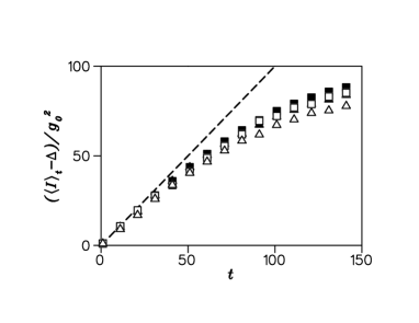
Figure 1: Mean value $(\langle I\rangle_{t}-\Delta)/g_{0}^{2}$ as a function of time $t$. Squares and triangles correspond to $(\hbar,g_{0})$=$(1,2)$ and $(2,3)$, full and empty symbols to $\Delta=0$ and $50$. The straight dashed line coresponds to the classical diffusion law $\langle I\rangle_{t}=\Delta+g_{0}^{2}t$.

IV.2 Zero-Harmonic Evolution and Quantum Diffusion

According to Eq. (10), the zero amplitude $W_{0}(I;t)$ is determined as

$$W_{0}(I;t)=\frac{2}{\hbar}\,e^{-\frac{2}{\hbar}I}\sum_{n=0}^{\infty}(-1)^{n}L_{n}\left(4I/\hbar\right)\langle n|{\hat{\rho}}(t)|n\rangle$$ (39)

by the diagonal matrix elements of the density operator. Our numerical simulations (see Fig. 2) show that these matrix elements decay along the main diagonal on average exponentially at any moment $t$ after a short initial interval (see below). Neglecting fluctuations we therefore assume that

$$\begin{array}[]{c}\rho_{nn}(t)=\langle n|{\hat{\rho}}(t)|n\rangle=\int d^{2}\overset{\circ}{\alpha}\,{\cal P}(|\overset{\circ}{\alpha}|^{2})\Big{|}\langle n\big{|}{\hat{U}}(t)\big{|}\overset{\circ}{\alpha}\rangle\Big{|}^{2}=\\ \sum_{n^{\prime}=0}^{\infty}\rho_{n^{\prime}}\Big{|}\langle n\big{|}{\hat{U}}(t)\big{|}n^{\prime}\rangle\Big{|}^{2}=\left[1-e^{-\nu(t)}\right]\,e^{-\nu(t)n},\\ \end{array}$$ (40)

with a function $\nu(t)$ which depends on the system’s dynamics. The approximation is similar to coarse graining of the classical distribution function. Correspondingly,

$$W_{0}(I;t)=\frac{2}{\hbar}\tanh\left(\frac{\nu}{2}\right)\exp\left[-\frac{2}{\hbar}\tanh\left(\frac{\nu}{2}\right)\,I\right]\,.$$ (41)

The dependence on time of the mean value of a function $Q({\hat{I}})$ of the action operator ${\hat{I}}=\hbar{\hat{n}}$ is then computed with the help of the formula

$$\langle Q\rangle_{t}=\int_{0}^{\infty}dIQ(I)W_{0}(I;t)$$ (42)

where the phase-space image of the operator ${\hat{Q}}$ is calculated similarly to the zero harmonic amplitude $W_{0}(I;t)$ of the Wigner function (see Eq. (10)). For example the image of the operator ${\hat{G}}(\kappa)=e^{-\kappa{\hat{I}}}$, which generates the moments of the amplitude $W_{0}(I;t)$ is easily found to be

$$G(\kappa;I)=\frac{\,e^{\kappa\hbar/2}}{\cosh\left(\kappa\hbar/2\right)}\,\exp\left[-2\tanh\left(\kappa\hbar/2\right)\frac{I}{\hbar}\right]\,.$$ (43)

The mean value of the generating function of the action momenta is readily obtained from eq. (42)

$$\langle G(\kappa;I)\rangle_{t}=e^{\frac{\kappa\hbar}{2}}\,\frac{\sinh(\nu/2)}{\sinh(\nu/2+\kappa\hbar/2)}\,.$$ (44)

In particular, the mean action equals $\langle I\rangle_{t}=-\partial\langle G(\kappa;I)\rangle_{t}/\partial\kappa\big{|}_{\kappa=0}=\frac{\hbar}{2}\left[\coth\left(\frac{\nu}{2}\right)-1\right]$. This formula relates the function $\nu(t)$ to the evolution of the action, $e^{-\nu(t)}=\langle I\rangle_{t}/(\langle I\rangle_{t}+\hbar)$, and allows us to represent finally the coarse-grained amplitude of the zero harmonic in the form

$$W_{0}(I;t)=\frac{1}{\langle I\rangle_{t}+\frac{\hbar}{2}}\exp\left(-\frac{I}{\langle I\rangle_{t}+\frac{\hbar}{2}}\right)\,.$$ (45)

The time dependence of the mean action $\langle I\rangle_{t}$ is shown in Fig. 1

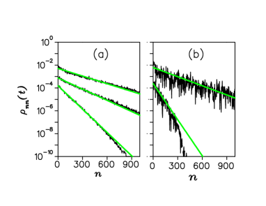
Figure 2: (color online) Distribution of the diagonal elements $\rho_{nn}(t)$ of the density matrix versus $n$, at $\hbar=1$, $g_{0}=2$. Left panel (a): mixed state ($\Delta=25$) and, from bottom to top, $t=10,30$, and $50$ (these curves are scaled by factors 0.01, 0.1 and 1, respectively). Right panel (b): pure state ($\Delta=0$), $t=10$ (bottom, scaled by a factor $0.01$) and $t=50$ (top). Straight lines show exponential fits, corresponding to the coarse-grained distribution (40).

IV.3 Evolution of Nonzero Momenta: Complexity of Quantum States

The paramount property of classical dynamical chaos is the exponentially fast structuring of the system’s phase space on finer and finer scales. In particular, the number ${\cal M}(t)$ of angular harmonics, that is the number of appreciably large harmonic’s amplitudes ${W^{(c)}}_{\,m}(I;t)$ in the Fourier expansion (13) of the classical distribution function $W^{(c)}(\alpha^{*},\alpha;t)$ grows exponentially in time. Namely ${\cal M}(t)\propto e^{t/\tau_{c}}$, where the characteristic time $\tau_{c}$ goes to infinite when the classical Lyapunov exponent vanishes. A simple consideration shows that the exponential regime cannot last long in the case of quantum dynamics. Indeed, in the terms of our auxiliary two-dimensional linear oscillator where the functions $e^{im\theta}$ are the eigenstates of the operator ${\hat{M}}$ defined in (26) the mean number of harmonics ${\cal M}(t)\sim\langle|n_{+}-n_{-}|\rangle_{t}\lesssim\langle N\rangle_{t}=\langle n_{+}+n_{-}\rangle_{t}\sim\langle I\rangle_{t}/\hbar\,.$ Therefore the exponential upgrowth is possible only for $e^{t/\tau_{c}}<\langle I\rangle_{t}/\hbar$, namely for a time $t\lesssim t_{E}=\tau_{c}\ln\frac{\langle I\rangle_{t}}{\hbar}\,.$ Since the mean action increases only linearly in time, $t_{E}$ is basically the Ehrenfest time Berman78 , logarithmically short in $\hbar$.

In order to ascertain how complex the quantum state became by the time $t$ we use as a probe a phase plane rotation by the angle $\delta\theta\equiv\xi$. Such a rotation is generated by the unitary transformation ${\hat{P}}(\xi)=e^{-i\xi{\hat{n}}}$ of the density matrix ${\hat{\rho}(t)}$. The effect of such perturbation, as mentioned above, is characterized by the Peres fidelity (4).

From the second line of Eq. (4) we obtain

$$F(\xi;t)=\sum_{n,n^{\prime}=0}^{\infty}\cos[\xi(n^{\prime}-n)]\frac{\Big{|}\langle n^{\prime}\big{|}{\hat{\rho}}(t)\big{|}n\rangle\Big{|}^{2}}{\sum_{k=0}^{\infty}\langle k\big{|}{\hat{\rho}}^{2}(t)\big{|}k\rangle}\,.$$ (46)

The diagonal ($n^{\prime}=n$) contribution

$$F_{0}(t)=\sum_{n=0}^{\infty}\frac{\Big{|}\langle n\big{|}{\hat{\rho}}(t)\big{|}n\rangle\Big{|}^{2}}{\sum_{k=0}^{\infty}\langle k\big{|}{\hat{\rho}}^{2}(t)\big{|}k\rangle}$$ (47)

does not depend on $\xi$. Taking into account that $F(\xi=0;t)=1$, we relate this contribution to the non-diagonal part of the density operator:

$$F_{0}(t)=1-2\sum_{n^{\prime}>n=0}^{\infty}\frac{\Big{|}\langle n^{\prime}\big{|}{\hat{\rho}}(t)\big{|}n\rangle\Big{|}^{2}}{\sum_{k=0}^{\infty}\langle k\big{|}{\hat{\rho}}^{2}(t)\big{|}k\rangle}.$$ (48)

After substitution of this expression into (46) we obtain

$$F(\xi;t)=1-2\sum_{m=1}^{\infty}\sin^{2}\left(\xi m/2\right)\mathcal{W}_{m}(t),$$ (49)

where

$$\mathcal{W}_{m}(t)=(2-\delta_{m0})\sum_{n=0}^{\infty}\frac{\Big{|}\langle n+m\big{|}{\hat{\rho}}(t)\big{|}n\rangle\Big{|}^{2}}{\sum_{n^{\prime}=0}^{\infty}\langle n^{\prime}\big{|}{\hat{\rho}}^{2}(t)\big{|}n^{\prime}\rangle}\,.$$ (50)

Since

$$\begin{array}[]{c}\sum_{n=0}^{\infty}\langle n\big{|}{\hat{\rho}}^{2}(t)\big{|}n\rangle=\sum_{n=0}^{\infty}\langle n\big{|}{\hat{\rho}}(t)\big{|}n\rangle^{2}+\\ 2\sum_{m=1}^{\infty}\sum_{n=0}^{\infty}\Big{|}\langle n+m\big{|}{\hat{\rho}}(t)\big{|}n\rangle\Big{|}^{2},\end{array}$$ (51)

we can convert Eq. (50) into

$$\begin{array}[]{c}{\mathcal{W}_{m}(t)}=\\ \frac{(2-\delta_{m0})\sum_{n=0}^{\infty}{\Big{|}\langle n+m\big{|}{\hat{\rho}}(t)\big{|}n\rangle\Big{|}^{2}}\Big{/}{\sum_{n^{\prime}=0}^{\infty}\rho_{n^{\prime}n^{\prime}}^{2}(t)}}{1+2\sum_{m=1}^{\infty}\sum_{n=0}^{\infty}\Big{|}\langle n+m\big{|}{\hat{\rho}}(t)\big{|}n\rangle\Big{|}^{2}\Big{/}{\sum_{n^{\prime}=0}^{\infty}\rho_{n^{\prime}n^{\prime}}^{2}(t)}},\end{array}$$ (52)

where $\rho_{nn}(t)$ is a shorthand notation for $\langle n\big{|}{\hat{\rho}}(t)\big{|}n\rangle$.

Equivalently, one can express ${\mathcal{W}_{m}(t)}$ in terms of the amplitudes (15) of the Wigner function:

$$\begin{array}[]{c}\mathcal{W}_{m}(t)=\\ \frac{(2-\delta_{m0})\int_{0}^{\infty}dI\big{|}W_{m}(I;t)\big{|}^{2}\big{/}\int_{0}^{\infty}dIW_{0}^{2}(I;t)}{1+2\sum_{m=1}^{\infty}\int_{0}^{\infty}dI\big{|}W_{m}(I;t)\big{|}^{2}\big{/}\int_{0}^{\infty}dIW_{0}^{2}(I;t)}\,.\\ \end{array}$$ (53)

The completeness condition

$$\begin{array}[]{c}\sum_{n=0}^{\infty}\frac{(n+m)!}{n!}L_{n}^{m}(4I/\hbar)L_{n}^{m}(4I^{\prime}/\hbar)=\\ \frac{\hbar}{4}\left(4I/\hbar\right)^{-m}e^{4I/\hbar}\delta(I-I^{\prime})\end{array}$$ (54)

has been taken into account in deriving formula (53). Similarly to Eq. (12), expression (53) remains valid in the classical limit, provided that the harmonics of the classical distribution function are used.

Since the normalization condition $\sum_{m}\mathcal{W}_{m}(t)=1$ holds, the quantities $\mathcal{W}_{m}(t)$, $m\geq 0$ give the probability distribution over the harmonic’s numbers $m$. Now, in the spirit of the linear response theory, we consider an infinitesimally small rotation angle $\xi\rightarrow 0$ and hold only the linear term of the power expansion of the density operator. The Eq. (49) reduces then to

$$\begin{array}[]{c}F(\xi;t)\approx 1-\frac{1}{2}\xi^{2}\,\langle m^{2}\rangle_{t}\,,\\ \langle m^{2}\rangle_{t}=-\frac{d^{2}F(\xi;t)}{d\xi^{2}}\Big{|}_{\xi=0}=\sum_{m=1}^{\infty}m^{2}\mathcal{W}_{m}(t)\,.\end{array}$$ (55)

Numerical simulations (see Fig. 3) show that, apart from small fluctuations, the distribution $\mathcal{W}_{m}(t)$ decreases with $m$ monotonically and exponentially. Therefore the quantity $\sqrt{\langle m^{2}\rangle}_{t}$ gives an estimate of the number ${\cal M}$ of harmonics developed up to time $t$ and can be considered as a suitable measure of complexity of the Wigner function at the time $t$.

According to the first line of Eq. (4), the same fidelity can, alternatively, be presented in the form

$$\begin{array}[]{c}F(\xi,t)=\sum_{n,n^{\prime}=0}^{\infty}\frac{\rho_{n}\rho_{n^{\prime}}}{\sum_{k=0}^{\infty}\rho_{k}^{2}}\Big{|}\langle n\big{|}e^{-i\xi{\hat{n}}(t)}\big{|}n^{\prime}\rangle\Big{|}^{2}=\\ 1-\xi^{2}\,\left[\overline{\chi_{2}(t)}-2\overline{\phi(t)}\right]+O({\xi}^{4})\end{array}$$ (56)

where the quantity

$$\overline{\chi_{2}(t)}=\sum_{n}\frac{\rho_{n}^{2}}{\sum_{n^{\prime}}\rho_{n^{\prime}}^{2}}\left(\langle n|{\hat{n}}^{2}(t)|n\rangle-\langle n|{\hat{n}}(t)|n\rangle^{2}\right)$$ (57)

is the weighted-mean value of the standard deviation of the excitation numbers at the moment $t$ whereas $\overline{\phi(t)}$ is similar weighted-mean value of the cumulative contribution

$$\phi(t)=\sum_{m=1}^{\infty}\left(1+\hbar/\Delta\right)^{-m}\,\big{|}\langle n+m|{\hat{n}}(t)|n\rangle\big{|}^{2}$$ (58)

of the off-diagonal matrix elements. Comparing now the $\xi^{2}$-terms in the both equivalent representations (55) and (56) of the fidelity we arrive at the following significant exact relation between the time behavior of the mean number of harmonics (which characterizes the complexity) on the one hand and of the excitation numbers on the other hand

$$\langle m^{2}\rangle_{t}=2\left[\overline{\chi_{2}(t)}-2\overline{\phi(t)}\right].$$ (59)

The negative second contribution which appears only in the case of mixed initial states reduces the number of harmonics.

Figure 3: Distribution of harmonics $\mathcal{W}_{m}(t)$ as a function of $m$, with parameter values as in Fig. 2.

V Quantum Reversibility: the Fidelity

To explore the reversibility of the quantum dynamics we consider now the perturbation angle $\xi$ as a free parameter and investigate the differences between the initial and reversed states as a function of $\xi$. To this end we first analyze the fidelity $F(\xi;t)$ at an arbitrary moment $t$ as a function of $\xi$.

Using Eq. (49), we can expand $F(\xi,t)$ in terms of the even moments $\langle m^{2k}\rangle$ ($k=1,2,...$) of the probability distribution (50)

$$F(\xi,t)=1-\sum_{k=1}^{\infty}(-1)^{k+1}\frac{\xi^{2k}}{(2k)!}\langle m^{2k}\rangle_{t}.$$ (60)

We remark that, due to the exponential decay (as a function of m) of the distribution $\mathcal{W}_{m}(t)$, all moments $\langle m^{2k}\rangle_{t}$ are finite.

On the other hand, the expansion of the general expression (56) over the parameter $\xi$ contains on- and off-diagonal matrix elements of the powers of the operator ${\hat{I}}(t)=\hbar\,{\hat{n}}(t)$ and therefore connect the Peres fidelity to the action evolution. Both the equivalent representations (60) and (56) will be exploited below.

V.1 Pure Coherent Initial State

The theoretical analysis is especially easy to carry out in the simple case of the (pure) ground initial state $\rho_{n}=\delta_{n0}$. The expression (56) reduces then to

$$F(\xi,t)=\big{|}\langle 0|{\hat{P}(\xi,t)}|0\rangle\big{|}^{2}=\Big{|}\langle 0|\,e^{-i\xi{\hat{n}}(t)}\,|0\rangle\Big{|}^{2}\,.$$ (61)

This specific initial state is the isotropic coherent state $|\overset{\circ}{\alpha}=0\rangle$ which corresponds to the distribution ${\cal P}(|\overset{\circ}{\alpha}|^{2})=\delta^{(2)}(\overset{\circ}{\alpha})$ in Eq. (36). After first few kicks, a state of practically general form is produced.

Making use of the cumulant expansion we obtain

$$F(\xi;t)=\exp\left[-2\sum_{l=1}^{\infty}\frac{(-1)^{l-1}}{(2l)!}\xi^{2l}\chi_{2l}(t)\right],$$ (62)

where the cumulants (connected momenta) are

$$\begin{array}[]{c}\chi_{2}(t)=\langle 0|\left({\hat{n}}(t)-\langle 0|{\hat{n}}(t)|0\rangle\right)^{2}|0\rangle,\\ \chi_{4}(t)=\langle 0|\left({\hat{n}}(t)-\langle 0|{\hat{n}}(t)|0\rangle\right)^{4}|0\rangle-\\ 3\left[\langle 0|\left({\hat{n}}(t)-\langle 0|{\hat{n}}(t)|0\rangle\right)^{2}|0\rangle\right]^{2},\\ \end{array}$$ (63)

and so on. Correspondingly, $L(\xi;t)\equiv-\ln F(\xi;t)=\xi^{2}\chi_{2}(t)-\frac{1}{12}\xi^{4}\chi_{4}(t)+...\,$. At a given time $t$ we can retain only the lowest cumulant, $L(\xi;t)\approx\xi^{2}\chi_{2}(t)$, as long as the perturbation strength $\xi\lesssim 2\sqrt{3\chi_{2}(t)/\chi_{4}(t)}$. However, as shown in Fig. 4, this approximation fails for larger values of $\xi$.

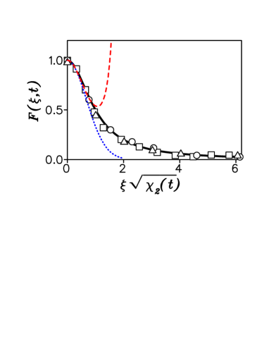
Figure 4: (color online) Fidelity $F(\xi,t)$ versus perturbation strength $\xi$, at $\hbar=0.25$, $g_{0}=2$ at three different times: $t=5,\sqrt{\chi_{2}(t)}=80$ (squares); $t=25,\sqrt{\chi_{2}(t)}=384$ (circles); $t=75,\sqrt{\chi_{2}(t)}=1010$ (triangles). The dotted and dashed curves show decay of the r.h.s. in Eq. (62) with, respectively, only the lowest and the two lowest terms of the cumulant expansion being kept. The full curve corresponds to the theoretical prediction of the second line in Eq. (66).

To go beyond such a restricted range of values of the parameter $\xi$ we observe that the amplitude $f(\xi;t)=\langle 0|e^{-i\xi{\hat{n}}(t)}|0\rangle$ can be readily represented as

$$f(\xi;t)=\sum_{n=0}^{\infty}w_{n}(t)\,e^{-i\xi n},$$ (64)

where $w_{n}(t)\equiv\langle n|{\hat{\rho}}(t)|n\rangle=\big{|}\langle n|{\hat{U}}(t)|0\big{|}^{2}$ is the excitation number probability distribution.

The probability $w_{n}(t)$ exhibits larger fluctuations as a function of $n$ than those in the case of broad initial mixtures (compare the two panels of Fig. 2 obtained for pure (right) and mixed (left) initial distributions). However, at any given time $t$ larger than the Ehrenfest time $w_{n}(t)$ decays, on average, exponentially. Assuming, similarly to (40), the exponential ansatz $w_{n}(t)\approx\left[1-e^{-\lambda(t)}\right]\,e^{-\lambda(t)n}$, we obtain

$$w_{n}(t)\approx\frac{1}{\langle n\rangle_{t}+1}\,\left[\frac{\langle n\rangle_{t}}{\langle n\rangle_{t}+1}\right]^{n},$$ (65)

where $\langle n\rangle_{t}$ is the mean excitation number at the moment $t$. The approximation (65) leads to the result

$$\begin{array}[]{c}F(\xi;t)\approx\frac{1}{1+4\langle n\rangle_{t}\left(\langle n\rangle_{t}+1\right)\,\sin^{2}(\xi/2)}=\\ \frac{1}{1+4\chi_{2}(t)\,\sin^{2}(\xi/2)}\approx\frac{1}{1+\xi^{2}\chi_{2}(t)}\,.\end{array}$$ (66)

In the second line we have taken into account that approximation (65) implies the following relation:

$$\chi_{2}(t)\equiv\langle 0|n^{2}|0\rangle_{t}-\langle 0|n|0\rangle_{t}^{2}\approx\langle n\rangle_{t}\left(\langle n\rangle_{t}+1\right).$$ (67)

(Let us remind in this connection that we have chosen $\overset{\circ}{\alpha}=0$). Opposite to the exact relation $\chi_{2}(t)=\frac{1}{2}\langle m^{2}\rangle_{t}$ (see eq. (59)) the relation eq. (67) is valid only after the Ehrenfest time $t_{E}$. Notice that accordingly to the first line in Eq. (66) $F(2\pi;t)=F(0;t)=1$, as expected since rotation by the angle $\xi=2\pi$ is just the identity operation.

Fig. 4 shows that the fidelity decay is nicely described by the analytical formula (66). It is also clearly seen that the fidelity almost vanishes already at very small values of the parameter $\xi$, so that the approximation given in the second line of Eq. (66) works quite well. We can therefore conclude that in the considered case of the pure ground initial state only the lowest cumulant $\chi_{2}$ determines the overall decay of the fidelity, whereas the higher ones are responsible for the fluctuations in the decay law.

Using the above exponential ansatz, the expression (50) for the probability distribution $\mathcal{W}_{m}(t)$ simplifies to

$$\begin{array}[]{c}\mathcal{W}_{m}(t)=(2-\delta_{m0})\sum_{n=0}^{\infty}w_{n+m}(t)\,w_{n}(t)\\ \approx\frac{2-\delta_{m0}}{2\langle n\rangle_{t}+1}\,\left[\frac{\langle n\rangle_{t}}{\langle n\rangle_{t}+1}\right]^{m},\end{array}$$ (68)

so that this distribution decays with the same slope $\lambda(t)$ as the distribution of the excitation numbers (65). Together with Eq. (67) this yields the following relation:

$$\langle m^{2}\rangle_{t}=2\,\chi_{2}(t)\approx 2\langle n\rangle_{t}\,(\langle n\rangle_{t}+1)\,.$$ (69)

Therefore, after an initial interval of order of the Ehrenfest time, the number of harmonics of the Wigner function increases with time in the same manner as the excitation number, not faster than linearly. Notice also that, as it should be, substitution of the expression (68) in the general formula (49) leads again to the same result (66).

The relatively slow dependence of $F(\xi;t)$ and the number of harmonics ${\cal M}(t)=\sqrt{\langle m^{2}\rangle_{t}}$ on time, which follows from expressions (66) and (69) should be juxtaposed with the classical behavior dictated by the exponential instability of the classical dynamics. The latter manifests itself, in particular, in the exponential growth of the number of harmonics of the classical phase-space distribution function $W_{c}(\alpha^{*},\alpha;t)$. To accomplish such a comparison we solve the classical Liouville equation with the initial phase space distribution $W_{c}(\alpha^{*},\alpha;0)=\frac{1}{\delta}\,e^{-\frac{|\alpha|^{2}}{\delta}}$ of size $\delta$ which coincides, for a given value of $\hbar$, with the size $\hbar/2$ of the Wigner function corresponding to the initial quantum ground state ${\hat{\rho}}(0)=|0\rangle\langle 0|$. The quantum to classical transition is explored by keeping $\delta$ constant and considering, for smaller and smaller values of $\hbar$, initial incoherent mixtures (38) of size $\delta=\Delta+\hbar/2$. A numerical illustration of such a procedure is presented in Fig. 5. The exponential increase of $\langle m^{2}\rangle_{t}$ up to the Ehrenfest time is clearly seen. After that time, a much slower power-law increase follows, in accordance, for pure states,with the relation (69). Such a behavior is consistent with the findings reported in the Refs. gu ; brumer .

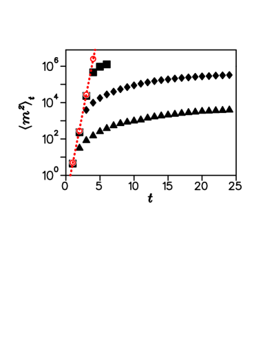
Figure 5: (color online) $\langle m^{2}\rangle_{t}$ versus $t$, at $g_{0}=1.5$, $\delta=0.5$. Squares, diamonds and triangles correspond to $\hbar=0.01,0.1$ and 1. In this latter case, the initial condition corresponds to the ground state, $\hat{\rho}(0)=|0\rangle\langle 0|$. Empty circles refer to classical dynamics and the dashed line is an exponential fit to these data, $\langle m^{2}\rangle_{t}=\exp(a+bt)$, with $a\approx-2.9$ and $b\approx 4.4$.

Figure 6: Distribution $\mathcal{W}_{m}$ of harmonics at times smaller than the Ehrenfest time, for parameter values $\hbar=0.01$, $g_{0}=1.5$. Data at $t=1$ and $t=3$ are scaled by a factor $0.1$.

The first relation in Eq. (69) allows us to directly connect the Peres fidelity after the Ehrenfest time with the, characterized by the mean number $\sqrt{\langle m^{2}\rangle_{t}}$ of harmonics, complexity of the Wigner function at time $t$:

$$\begin{array}[]{c}F(\xi;t)\approx\frac{1}{1+\frac{1}{2}\xi^{2}\langle m^{2}\rangle_{t}}=\\ \\ 1-\sum_{k=1}^{\infty}(-1)^{k+1}\xi^{2k}(\langle m^{2}\rangle_{t})^{k}\,.\end{array}$$ (70)

More than that, comparing the terms of the two expansions, (60) and (70), the former of which is exact for any time including times shorter or of the order of the Ehrenfest time, we see that also the latter would be always correct if

$$\langle m^{2k}\rangle_{t}=\frac{(2k)!}{2^{k}}(\langle m^{2}\rangle_{t})^{k}\,.$$ (71)

Such a relation is characteristic of the exponentially decaying distribution. Numerical data presented in Fig. 6 support such a conjecture. It follows then that in accordance with the different growth of the number of harmonics before and after the Ehrenfest time (see Fig. 5), the slope of the $m$-dependence of the distribution $\mathcal{W}_{m}(t)$ is drastically different inside and outside the Ehrenfest time scale. This slope decreases exponentially with $t$ in the first case and not faster than linearly in the second.

VI Quantum Reversibility: the Time-Reversed State.

In this section, we study in detail the phase-space structure of the time-reversed state characterized by the harmonics content of the Wigner function in dependence on the perturbation strength $\xi$ and the reversal time $T$.

Generally, the Peres fidelity $F(\xi;T)$, as it appeares in the first line of Eq. (12), is sensitive only to the distortion of the zero harmonic of the reversed Wigner function or, equivalently, to the redistribution of the excitation numbers. Utilizing the first line of Eq. (4) we obtain in the terms of the density matrix

$$\begin{array}[]{c}F(\xi;T)=\sum_{n=0}^{\infty}\frac{\rho_{n}}{\sum_{n^{\prime}=0}^{\infty}\rho_{n^{\prime}}^{2}}\langle n\big{|}{\hat{\tilde{\rho}}}(0|T,\xi)\big{|}n\rangle\approx\\ 2\sum_{n=0}^{\infty}e^{-\frac{\hbar}{\Delta}\,n}\,\langle n\big{|}{\hat{\tilde{\rho}}}(0|T,\xi)\big{|}n\rangle,\,\,\,(\Delta\gg\hbar),\end{array}$$ (72)

where only the diagonal matrix elements

$$\begin{array}[]{c}\langle n|{\hat{\tilde{\rho}}}(0|T,\xi)|n\rangle=\sum_{n^{\prime}=0}^{\infty}\rho_{n^{\prime}}\,\Big{|}\langle n\big{|}{\hat{P}}(\xi,T)\big{|}n^{\prime}\rangle\Big{|}^{2}=\\ \rho_{n}\,\Big{|}\langle n\big{|}{\hat{P}}(\xi,T)\big{|}n\rangle\Big{|}^{2}+\\ \sum_{n^{\prime}=0}^{\infty}\left(1-\delta_{nn^{\prime}}\right)\rho_{n^{\prime}}\,\Big{|}\langle n\big{|}\left({\hat{P}}(\xi,T)-1\right)\big{|}n^{\prime}\rangle\Big{|}^{2}\end{array}$$ (73)

of the reversed density matrix are present. Only the term which stays in the second line of this equation remains in the limit $\xi\rightarrow 0$. This limit is shown with the dotted line in the Fig. 8.

The effect of perturbation shows up first in the second order with respect to the perturbation parameter $\xi$. Expanding in Eq. (73) the operator ${\hat{P}}(\xi,T)=e^{-i\,\xi{\hat{n}}(T)}$ up to the correction of this order we find

$$\begin{array}[]{c}\langle n|{\hat{\tilde{\rho}}(0|T,\xi)}|n\rangle\approx\\ \rho_{n}\left[1-\xi^{2}\left(\langle n|{\hat{n}}^{2}(T)|n\rangle-\langle n|{\hat{n}}(T)|n\rangle^{2}\right)\right]+\\ \xi^{2}\sum_{n^{\prime}\neq n}\rho_{n^{\prime}}\big{|}\langle n^{\prime}|{\hat{n}}(T)|n\rangle\big{|}^{2}\end{array}$$ (74)

which leads to Eq. (56) again.

The fidelity (72) consists of two different contributions $\overline{F_{n}(\xi;T)}^{(n)}+\overline{F^{(m)}(\xi;T)}$ one of which

$$\overline{F_{n}(\xi;T)}^{(n)}\equiv\sum_{n=0}^{\infty}\frac{\rho_{n}^{2}}{\sum_{k=0}^{\infty}\rho_{k}^{2}}\Big{|}\langle n\big{|}{\hat{P}}(\xi,T)\big{|}n\rangle\Big{|}^{2}$$ (75)

is the weighted mean of pure state fidelities, whereas the off-diagonal contribution

$$\begin{array}[]{c}\overline{F^{(m)}(\xi;T)}=\\ 2\sum_{n=0}^{\infty}\frac{\rho_{n}^{2}}{\sum_{k=0}^{\infty}\rho_{k}^{2}}\sum_{m=1}^{\infty}e^{-\frac{\hbar}{\Delta}m}\Big{|}\langle n+m\big{|}{\hat{P}}(\xi,T)\big{|}n\rangle\Big{|}^{2}\end{array}$$ (76)

is specific for mixed initial states.

However, the important information on the harmonics that survived the backward evolution is absent in the fidelity (72). To find their number and the corresponding distribution $\tilde{\mathcal{W}}_{m}(0|\,\xi;T)$ we perturb the reversed density matrix ${\hat{\tilde{\rho}}}(0|T,\xi)$ by means of the probing operation ${\hat{P}}(\xi^{\prime})=e^{-i\xi^{\prime}{\hat{n}}}$, with a new infinitesimally small rotation angle $\xi^{\prime}$ . In the same manner as in Sec. IV.3 we obtain (compare with (55))

$$\langle{\tilde{m}}^{2}(\xi;T)\rangle=\sum_{m=1}^{\infty}m^{2}\tilde{\mathcal{W}}_{m}(0|\,\xi;T),$$ (77)

where

$$\begin{array}[]{c}\tilde{\mathcal{W}}_{m}(0|\,\xi;T)=(2-\delta_{m0})\sum_{n=0}^{\infty}\frac{\Big{|}\langle n+m\big{|}{\hat{\tilde{\rho}}}(0)\big{|}n\rangle\Big{|}^{2}}{\sum_{k=0}^{\infty}\langle k\big{|}{\hat{\tilde{\rho}}}^{2}(0)\big{|}k\rangle}=\\ \frac{(2-\delta_{m0})\sum_{n=0}^{\infty}{\Big{|}\langle n+m\big{|}{\hat{\tilde{\rho}}}(0)\big{|}n\rangle\Big{|}^{2}}\Big{/}{\sum_{k=0}^{\infty}{\tilde{\rho}}_{kk}^{2}(0)}}{1+2\sum_{m=1}^{\infty}\sum_{n=0}^{\infty}\Big{|}\langle n+m\big{|}{\tilde{\rho}}(0)\big{|}n\rangle\Big{|}^{2}\Big{/}{\sum_{k=0}^{\infty}{\tilde{\rho}}_{kk}^{2}(0)}}=\\ \frac{(2-\delta_{m0})\int_{0}^{\infty}\!dI\big{|}\tilde{W}_{m}(I;0)\big{|}^{2}\Big{/}\int_{0}^{\infty}\!dI\,\tilde{W}_{0}^{2}(I;0)}{1+2\sum_{m=1}^{\infty}\int_{0}^{\infty}\!dI\big{|}\tilde{W}_{m}(I;0)\big{|}^{2}\Big{/}\int_{0}^{\infty}\!dI\,\tilde{W}_{0}^{2}(I;0)}\,.\end{array}$$ (78)

We have used the shorthands ${\hat{\tilde{\rho}}(0|T,\xi)}\Rightarrow{\hat{\tilde{\rho}}(0)}$ and $\tilde{W}_{m}(I;0|T,\xi)\Rightarrow\tilde{W}_{m}(I;0)$ in these formulae.

VI.1 Pure Initial State

We note now that, according to the first line of the relation (70), in the special case of a pure initial state the crossover

$$F(\xi,T)\approx\left\{\begin{array}[]{c}1,\qquad\mbox{if}\quad\xi\ll\xi_{c}(T),\\ \frac{2}{\xi^{2}\,\langle m^{2}\rangle_{T}},\qquad\mbox{if}\quad\xi\gg\xi_{c}(T)\end{array}\right.$$ (79)

from good to poor reversibility takes place near the critical value $\xi_{c}(T)\equiv\sqrt{2/\langle m^{2}\rangle_{T}}$ of the strength $\xi$ of the perturbation. The validity of the formula (70) for pure initial states is illustrated by the numerical data plotted in Fig. 7.

The numerical results presented in Fig. 5 imply that the fidelity $F(\xi,T)$ decays as a function of the reversal time $T$ the faster (approaching the exponential decay typical of the classical chaotic dynamics benenti02 ) the closer the motion is to the semi-classical region. Within the interval $T\lesssim$ the Ehrenfest time the decay is exponential with the rate $1/\tau_{c}$ which describes the classical exponential proliferation of the number of harmonics and does not depend on the perturbation constant $\xi$.

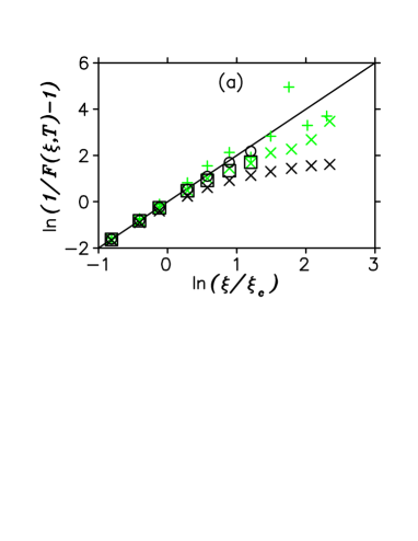
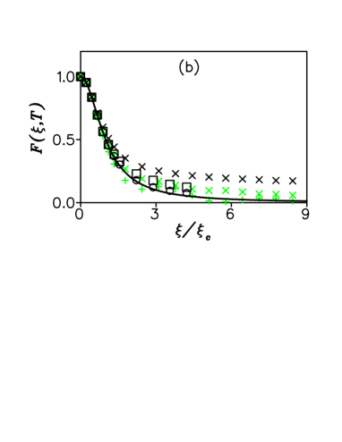
Figure 7: (color online) Fidelity $F(\xi;T)$ versus the scaled variable $\xi/{\xi}_{c}(T)$. Data correspond to: (i) $\hbar=1,g_{0}=2$; light pluses: $T=10$, $\Delta=0$; light and black crosses: $T=50$, $\Delta=0$ and 25; (ii) $\hbar=0.1,g_{0}=1.5$, $\Delta=0.45$ and $T=20$; (black open circles); (iii) $\hbar=0.01,g_{0}=1.5,\Delta=0.5$ and $T=2$. (black open squares). The curves show the theoretical prediction of Eq. (70).

With regard to the number of harmonics of the time-reversed state, expression (78) reduces, for a pure initial state, (compare with Eq. (68)) to

$$\tilde{\mathcal{W}}_{m}(0|\,\xi;T)=(2-\delta_{m0})\sum_{n=0}^{\infty}{\tilde{w}}_{n+m}(\xi;T)\,{\tilde{w}}_{n}(\xi;T),\\$$ (80)

where

$${\tilde{w}}_{n}(\xi;T)\equiv\tilde{\rho}_{nn}(0|T,\xi)=\big{|}\langle n|e^{-i\xi{\hat{n}}(T)}|0\rangle\big{|}^{2}\,.$$ (81)

In particular ${\tilde{w}}_{0}(\xi;T)=F(\xi;T)$ (see Eq. (61)).

We expect again an overall exponential decay of the excitation number probability distribution: ${\tilde{w}}_{n\geq 1}(\xi;T)\approx A(\xi;T)\,e^{-{\tilde{\nu}(T)}n}$. This assumption is well confirmed by numerical simulations, examples of which are presented in Figs. 8, 9 where exponential decays of both the $n$-and $m$-distributions ${\tilde{w}}_{n\geq 1}(\xi;T),\,\,\tilde{\mathcal{W}}_{m}(0|\,\xi;T)$ is demonstrated in agreement with Eq. (80). It is clearly seen that the decay rate $\tilde{\nu}(T)$ does not depend on the perturbation strength $\xi$. The normalization condition $\sum_{n=0}^{\infty}{\tilde{w}}_{n}=1$ defines the normalization constant $A(\xi;T)$ thus connecting the $n$-distribution with the fidelity

$${\tilde{w}}_{n\geq 1}(\xi;T)=\left(1-F(\xi;T)\right)\,\left(e^{{\tilde{\nu}(T)}}-1\right)\,e^{{-\tilde{\nu}(T)}n}\,.$$ (82)

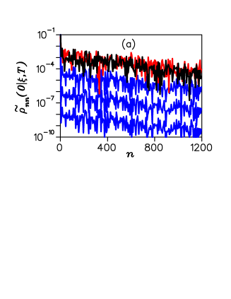
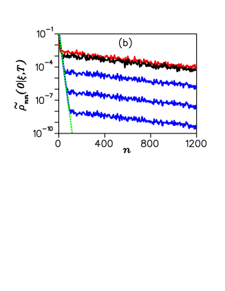
Figure 8: (color online) Decay of $\tilde{\rho}_{nn}(0|\xi,T)$ as a function of $n$, at $\hbar=1$, $g_{0}=2$ and $T=50$, for (a) pure ($\Delta=0$) and (b) mixed ($\Delta=5$) initial states. Curves from bottom to top correspond to different values of perturbation parameter $\xi=\xi_{c}\times 2^{l/2}$, $l=-9,-6,-3,0$ and $3$. The dotted line corresponds to the initial distribution $\rho_{nn}(0)=\frac{\hbar}{\Delta+\hbar}\,\left(\frac{\Delta}{\Delta+\hbar}\right)^{n}$.

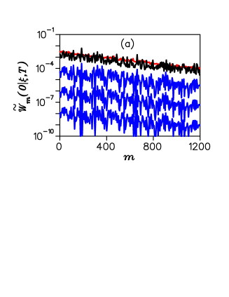
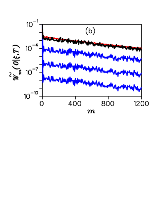
Figure 9: (color online) Decay of ${\tilde{\cal W}}_{m}(0|\xi,T)$ as a function of $m$, with $\Delta=0$ and the other parameter values as in Fig. 8.

A simple although a bit lengthy calculation connects, quite similarly to the relation expressed by Eqs. (67) and (69), the second moment of the distribution (80) to the fluctuations of the excitation numbers:

$$\begin{array}[]{c}\langle{\tilde{m}^{2}}(\xi;T)\rangle=2\left[\langle{\tilde{n}^{2}}(\xi;T)\rangle-\langle{\tilde{n}}(\xi;T)\rangle^{2}\right]=\\ 2\frac{\left(1-F(\xi;T)\right)\left(F(\xi;T)+e^{-{\tilde{\nu}(T)}}\right)}{\left(1-e^{-{\tilde{\nu}(T)}}\right)^{2}}\,.\\ \end{array}$$ (83)

Notice that the ratio of the first two moments of the distribution (80) calculated with the help of the parametrization (82)

$$\Lambda(T)\equiv\frac{\langle{\tilde{m}}(\xi;T)\rangle}{\langle{\tilde{m}^{2}}(\xi;T)\rangle}=\frac{\langle{\tilde{n}}(\xi;T)\rangle}{\langle{\tilde{n}^{2}}(\xi;T)\rangle}=\frac{1-e^{{-\tilde{\nu}(T)}}}{1+e^{{-\tilde{\nu}(T)}}}$$ (84)

does not depend on $\xi$ and is small if the reversal time $T$ is not too small. In this case $\tilde{\nu}(T)\approx 2\Lambda(T)\ll 1$.

When the perturbation parameter $\xi\ll\xi_{c}(T)$ so that the Peres fidelity (70) is close to 1, we obtain from Eq. (83) the ratio

$$\begin{array}[]{c}R(\xi,T)\equiv\frac{\langle{\tilde{m}^{2}}(\xi;T)\rangle}{\langle m^{2}\rangle_{T}}\approx\frac{1}{2}\left(\frac{\xi}{\Lambda(T)}\right)^{2}\\ =\frac{1}{2}\left(\frac{\xi_{c}(T)}{\Lambda(T)}\right)^{2}\,\left(\frac{\xi}{\xi_{c}(T)}\right)^{2},\end{array}$$ (85)

which characterizes the residual complexity of the reversed state. This ratio remains small and therefore the motion remains practically reversible as long as $\xi\ll\Lambda(T)$. For the parameters fixed in the top panel of Fig. 8 the ratio $\xi_{c}(T)/{\sqrt{2}\Lambda(T)}\approx 1.44$ so that the condition of reversibility looks as $\xi<0.69\,\xi_{c}(T)$ in reasonable agreement with the condition obtained above with the help of fidelity.

VI.2 Incoherent Initial Mixture

When the evolution starts with a mixed initial state the $\xi^{2}$-correction in the expansion (56) of the Peres fidelity contains along with the negative contribution defined by the weighted-mean value of the lowest cumulant $\overline{\chi_{2}(T)}$ (compare with Eq. (67)) an additional positive one. Still, the condition $\xi\lesssim{\xi}_{c}(T)$ holds as the criterion for the Peres fidelity to be close to one.

Contrary to the diagonal matrix elements (74), the off-diagonal elements of the density matrix are distorted already in the first order approximation,

$$\begin{array}[]{c}\langle n+m|{\hat{\tilde{\rho}}(0|T,\xi)}|n\rangle\approx\\ \rho_{n}\delta_{m0}+i\xi\langle n+m|{\hat{n}}(T)|n\rangle\,\rho_{n}\left(1-\frac{\rho_{n+m}}{\rho_{n}}\right)\,.\end{array}$$ (86)

As long as $\xi$ is small enough only the probability of zero harmonic $\tilde{\mathcal{W}_{0}}$ is close to unity whereas the probabilities of other harmonics are small as $\xi^{2}$:

$$\begin{array}[]{c}\tilde{\mathcal{W}}_{m\geqslant 1}(0|\,\xi;T)\approx\xi^{2}\,{\tilde{q}}_{m}(0|0,T),\\ \tilde{\mathcal{W}}_{0}(0|\,\xi;T)\approx 1-\xi^{2}\,{\tilde{q}}_{0}(0|0,T)\,,\end{array}$$ (87)

where

$$\begin{array}[]{c}{\tilde{q}}_{m\geqslant 1}(0|0,T)=\left[1-\left(\frac{\Delta}{\Delta+\hbar}\right)^{m}\right]^{2}\times\\ \Sigma_{n=0}^{\infty}\frac{\rho_{n}^{2}}{\sum_{k=0}^{\infty}\rho_{k}^{2}}|\langle n+m|{\hat{n}}(T)|n\rangle|^{2}\equiv d_{m}\times{\tilde{r}}_{m}(0|0,T)\end{array}$$ (88)

and

$${\tilde{q}}_{0}(0|0,T)=\sum_{m=1}^{\infty}{\tilde{q}}_{m}(0|0,T)\,.$$ (89)

If the initial mixture is wide, $\Delta\gg\hbar$, the pre-factor $d_{m}\approx\left(1-e^{-\frac{\hbar}{\Delta}m}\right)^{2}$ is small for all $m\lesssim\Delta/\hbar$. This explains the dip seen in Fig. 10 (above). At the same time, Fig. 10 (below) shows that the second factor ${\tilde{r}}_{m}(0|0,T)$ is very well described by an exponential. Therefore we suppose that

$$\begin{array}[]{c}{\tilde{q}}_{m}(0|0,T)=\frac{{\tilde{q}}_{0}(0|0,T)}{z(\mu)}\,d_{m}\,e^{-\mu(T)m}\,,\\ z(\mu)=\sum_{m=1}^{\infty}d_{m}\,e^{-\mu m}\,.\end{array}$$ (90)

To fix the two unknown functions ${\tilde{q}}_{0}(0|0,T)$ and $\mu(T)$ we calculate the moments

$$\begin{array}[]{c}\tilde{\mathfrak{m}}^{(k)}(T)=\sum_{m=1}^{\infty}m^{k}{\tilde{q}}_{m}(0|0,T)=\\ ={\tilde{q}}_{0}(0|0;T)\,\frac{1}{z(\mu)}\,\left(-\frac{d}{d\mu}\right)^{k}\,z(\mu)\,.\end{array}$$ (91)

Then

$$\begin{array}[]{c}{\tilde{q}}_{0}(0|0;T)=-\tilde{\mathfrak{m}}^{(1)}(T)\frac{z(\mu)}{z^{\prime}(\mu)}\,,\\ {\tilde{q}}_{m}(0|0;T)=-\frac{\tilde{\mathfrak{m}}^{(1)}(T)}{z^{\prime}(\mu)}\,d_{m}\,e^{-\mu m}\,,\end{array}$$ (92)

where the prime denotes differentiation with respect to the parameter $\mu$. Besides we obtain the connection

$$\Lambda(T)\equiv\frac{\tilde{\mathfrak{m}}^{(1)}(T)}{\tilde{\mathfrak{m}}^{(2)}(T)}=-\frac{z^{\prime}(\mu)}{z^{\prime\prime}(\mu)}\,,$$ (93)

which expresses the function $\mu(T)$ in the terms of the two lowest momenta. Under the condition $\Lambda\ll 1$, which is well justified by our numerical simulations, equation (93) can be solved analytically resulting in $\mu(T)\approx 2\Lambda(T)$. Thus the two lowest moments entirely fix the probability distribution $\tilde{\mathcal{W}}_{m}$.

Figure 10: (color online) Distribution ${\tilde{q}}_{m}$ (a) and exponential decay of the factor $\tilde{r}_{m}$ (b), for reversal times $T=50$ (bottom curves) and $T=100$ (top curves), at $\hbar=1$, $g_{0}=2$, $\Delta=200$. Straight lines correspond to $\exp(-2\Lambda m)$ [see Eq. (93)].

When the ratio $\xi/\xi_{c}(T)$ exceeds the unity, the dip in the probability distribution $\tilde{\mathcal{W}}_{m}(0|\,\xi;T)$ disappears and the following exponential fit works well for all nonzero harmonics (see Fig. 11):

$$\tilde{\mathcal{W}}_{m\geqslant 1}=\left(1-\tilde{\mathcal{W}}_{0}\right)\,(e^{\mu}-1)\,e^{-\mu m}\,.$$ (94)

As above we can express ${\tilde{\mathcal{W}}}_{0}$ and $\mu$ in terms of two moments $\langle{\tilde{m}}^{k}\rangle=\sum_{m=0}^{\infty}m^{k}{\tilde{\mathcal{W}}}_{m}$, $k=1,2$. Now we easily find that

$$\begin{array}[]{c}\tilde{\mathcal{W}}_{0}=1-\langle{\tilde{m}}\rangle\,\frac{2\Lambda}{1+\Lambda}\approx 1-2\langle{\tilde{m}}\rangle\,\Lambda\,,\\ \tilde{\mathcal{W}}_{m\geqslant 1}=\langle{\tilde{m}}\rangle\,\frac{4\Lambda^{2}}{1-\Lambda^{2}}\,\left(\frac{1-\Lambda}{1+\Lambda}\right)^{m}\approx 4\langle{\tilde{m}}\rangle\,\Lambda^{2}\,e^{-2\Lambda m}\end{array}$$ (95)

where $\Lambda(T)=\frac{\langle{\tilde{m}}\rangle}{\langle{\tilde{m}}^{2}\rangle}$.

Figure 11: (color online) Same as in Fig. 9 but starting from a mixed state with $\Delta=200$.

A large number $\sim 1/2\Lambda(T)$ of harmonics have in this case similar noticeable probabilities.

In Fig. 12 the ratio $R(\xi,T)=\langle{\tilde{m}(\xi,T)}^{2}\rangle/\langle m^{2}\rangle_{T}$ is plotted as a function of the parameter $\xi/\xi_{c}(T)$. When this parameter is small the ratio is also small and proportional to $\xi^{2}$. Since the fidelity $F(\xi;T)$ which describes the redistribution of the excitation numbers after the backward evolution is close to one under this condition, we conclude that the initial state is recovered with good accuracy and the motion is well reversible. On the contrary, when the perturbation strength $\xi$ exceeds the critical value $\xi_{c}(T)$ the fidelity becomes small and the residual number of harmonics gets even larger than the number of harmonics developed during the forward evolution. Therefore the evolution becomes irreversible.

Figure 12: Ratio $R(\xi,R)$ as a function of the parameter $\xi/\xi_{c}(T)$, at $\hbar=2$, $g_{0}^{2}=6$, $\Delta=50$, and $T=50$.

More precisely, for any reversal time $T$, there exists an interval $0<\xi<\xi_{c}(T)$ of the perturbation strength $\xi$, within which the quantum dynamics is approximately reversible. This interval, is defined by the rate of proliferation of the number of harmonics. In particular, this interval diminishes exponentially fast when the semiclassical domain is approached.

At last the detailed temporal pattern is presented in Figs. 13 of the backward evolution for both the excitation number (panel (a)) as well as the number of harmonics (panel (b)). It is clearly seen that the time interval $\Delta t$ during which the system passes in reversed order approximately the same sequence of the states, which it does while evolving forward, decreases as a function of the ratio $\xi/\xi_{c}(T)$. The existence of minimal deviation (or the time of maximal return) during the backward evolution has been stressed first in Kottos03 ; Kottos04 .

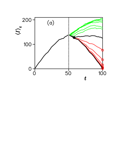
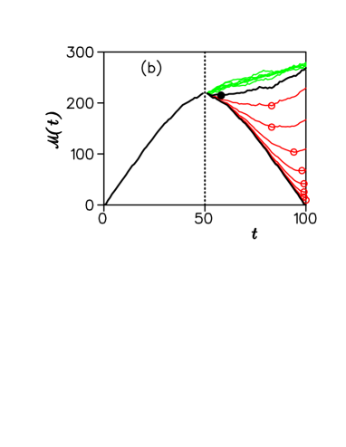
Figure 13: (color online) Reversibility properties of quantum dynamics, displayed by (a) $\langle I\rangle_{t}$ and (b) ${\cal M}(t)=\sqrt{\langle m^{2}\rangle_{t}}$ , for different values of the perturbation parameter: from bottom to top, $\xi=\xi_{c}\times\exp{(l/2)}$, $l=-8,\ldots,-1$, $l=0$ (thick black curve marked by the closed circle), and $l=1,\ldots,6$, at $\hbar=1$, $g_{0}=2$, $\Delta=1$. Circles indicate positions of the minima on the curves.

VII Summary

In this paper we have investigated the degree of stability and reversibility of the quantum dynamics of classically chaotic systems beyond the semi-classical domain. As a measure of complexity we have used the number ${\cal M}(t)=\sqrt{\langle m^{2}\rangle_{t}}$ of angular harmonics of the (initially isotropic) Wigner function $W(I,\theta;t)$, developed during the evolution for the time $t$. This number describes the system’s response to instantaneous rotation at that moment by an infinitesimal angle $\xi\to 0$. The number ${\cal M}(t)$ is found by calculating the distance between the perturbed (rotated) and unperturbed quantum distributions. We show that, in contrast to the classical chaotic motion where the number of harmonics grows exponentially, ${\cal M}_{c}(t)\sim e^{t/\tau_{c}}$ (with the rate $1/\tau_{c}$ increasing together with the Lyapunov exponent), the number of harmonics of the quantum Wigner function increases, after the Ehrenfest time, not faster than linearly. This reveals much weaker sensitivity of the quantum dynamics to perturbations than it is in the case of the classical dynamics.

The relatively weak response of quantum systems to external perturbations makes the quantum dynamics, to some extent, reversible unlike the practically irreversible classical chaotic dynamics. To quantify this statement we have analyzed the degree of recovery of the initial, generally incoherent, mixed state after the backward evolution of the quantum distribution $W(I,\theta;t)$, rotated by a finite angle $\xi$ at some reversal moment of time $t=T$. The lack of the perfect reversibility of the dynamics manifests itself by means of a redistribution of the excitation numbers and by the number ${\tilde{\cal M}}(0)$ of harmonics of the Wigner function, which remains after the backward evolution. Whereas the first effect is directly described by the Peres fidelity the second one is, in general, revealed with the help of an additional infinitesimal rotation of the reversed state. We have shown that there exists a critical value $\xi_{c}(T)=\sqrt{2}/{\cal M}(T)$ of the perturbation strength $\xi$ such that the initial state is well recovered if $\xi\ll\xi_{c}(T)$. Reversibility disappears when the perturbation angle exceeds this value. The interval of reversibility $0<\xi<\xi_{c}(T)$ exponentially shrinks while approaching the semi-classical domain.

Thus our analysis establishes a direct quantitative connection between the complexity of quantum phase-space distribution, reduced in comparison to the classical dynamics, and the degree of reversibility of the quantum dynamics.

References

- (1) D.L. Shepelyansky, Physica D 8, 208 (1983); G. Casati, B.V. Chirikov, I. Guarneri, and D.L. Shepelyansky, Phys. Rev. Lett. 56, 2437 (1986).
- (2) B.V. Chirikov, F.M. Izrailev, and D.L. Shepelyansky, Sov. Sci. Rev. C 2, 209 (1981).
- (3) Y. Gu, Phys. Lett. A 149, 95 (1990).
- (4) A.K. Pattanayak and P. Brumer, Phys. Rev. E 56, 5174 (1997); J. Gong and P. Brumer, Phys. Rev. A 68, 062103 (2003).
- (5) K.S. Ikeda, in Quantum chaos: between order and disorder, G. Casati and B.V. Chirikov (Eds.) (Cambridge University Press, 1995).
- (6) A. Peres, Phys. Rev. A 30, 1610 (1984).
- (7) Quantity (4) has been widely investigated in studies of the so-called quantum Loschmidt echo prosen . However, we would like to note that, similarly to Ref. heller and in contrast to other previous studies prosen , the backward evolution proceeds with the same Hamiltonian as the forward evolution and the perturbation acts instantaneously only at the reversal time .
- (8) A review on the quantum Loschmidt echo is provided by T. Gorin, T. Prosen, T.H. Seligman, and M. Žnidarič, Phys. Rep. 435, 33 (2006). Ph. Jacquod and C. Petitjean, preprint arXiv:0806.0987v1 [quant-ph] 5 Jun 2008
- (9) C. Petitjean, D.V. Bevilaqua, E.J. Heller, and Ph. Jacquod, Phys. Rev. Lett. 98, 164101 (2007).
- (10) R.J. Glauber, Phys. Rev. 131 2766 (1963).
- (11) G.S. Agarwal and E. Wolf, Phys. Rev. D 2, 2161 (1970); ibid. 2187 (1970).
- (12) J. Schwinger, Phys. Rev. 91, 728 (1953).
- (13) G.P. Berman, G.M. Zaslavsky, Physica A 91, 450 (1978); ibid. 97, 367 (1979).
- (14) V.V. Sokolov, Nonlinear Resonance of a Quantum oscillator prep. Inst. Nucl. Phys. Siberia Div. Acad. Sci USSR (1978); Teor. Mat. Fiz. 61, 128 (1984) [Sov. J. Theor. Math. 61, 104 (1985)].
- (15) V.V. Sokolov, G. Benenti, and G. Casati, Phys. Rev. E 75, 026213 (2007).
- (16) G. Benenti and G. Casati, Phys. Rev. E 65, 066205 (2002); G. Benenti, G. Casati, and G. Veble, Phys. Rev. E 67, 055202(R) (2003).
- (17) T. Kottos and D. Cohen, Europhys Lett. 61, 431 (2003).
- (18) Moritz Hiller, Tsampikos Kottos, Doron Cohen and Theo Geisel, Phys. Rev. Lett. 92 010402 (2004).