Iterative (“Turbo”) Multiuser Detectors for Impulse Radio Systems

Abstract

In recent years, there has been a growing interest in multiple access communication systems that spread their transmitted energy over very large bandwidths. These systems, which are referred to as ultra wide-band (UWB) systems, have various advantages over narrow-band and conventional wide-band systems. The importance of multiuser detection for achieving high data or low bit error rates in these systems has already been established in several studies. This paper presents iterative (“turbo”) multiuser detection for impulse radio (IR) UWB systems over multipath channels. While this approach is demonstrated for UWB signals, it can also be used in other systems that use similar types of signaling. When applied to the type of signals used by UWB systems, the complexity of the proposed detector can be quite low. Also, two very low complexity implementations of the iterative multiuser detection scheme are proposed based on Gaussian approximation and soft interference cancellation. The performance of these detectors is assessed using simulations that demonstrate their favorable properties.

Index Terms— Ultra wide-band (UWB), impulse radio (IR), iterative multiuser detection, soft interference cancellation.

I Introduction

In recent years, there has been a growing interest in ultra wide-band (UWB) systems, which resulted in the U.S. Federal Communications Commission (FCC) regulations that allow, under several restrictions, the widespread use of such systems. The common definition of UWB systems, which was adopted by the FCC as well, states that a system is a UWB system if both the absolute and the fractional bandwidths are large. The absolute bandwidth should be at least $0.5$ GHz, while the fractional bandwidth, which is the signal bandwidth divided by the carrier frequency, is at least $20\%$ [8]. UWB systems offer many advantages over narrow-band or conventional wide-band systems. Among these advantages are reduced fading margins, simple transceiver designs, low probability of detection, good anti-jam capabilities, and accurate positioning (see, [5, 33, 14], and references therein). The advantages of UWB technology have caused this technology to be considered for use as the physical layer of several applications; for example, the IEEE 802.15.4a wireless personal area network (WPAN) standard employs this technology as one of the signaling options [37].

There are many signaling methods for transmitting over UWB channels, and it is obvious that, apart from engineering difficulties, one can use any existing spread spectrum technique for transmitting over UWB channels [10, 32]. However, these difficulties might be quite significant, preventing the actual use of conventional spread-spectrum methods for transmitting over UWB channels. Consider, as an example, long-code direct-sequence code-division-multiple-access (DS-CDMA) systems. In these systems, implementing even the simplest detector, namely the matched filter detector, requires sampling of the received signal at least at the chip rate, which under the current regulations might be as large as $7.5$ GHz. Such sampling rates are difficult to achieve, and result in high power consumption.

In order to overcome some of the difficulties associated with UWB signaling, impulse radio (IR) systems, and especially time-hopping impulse radio (TH-IR) systems have been proposed as the preferred modulation scheme for UWB systems [26]. In TH-IR systems, a train of short pulses is transmitted, and the information is usually conveyed by either the polarity or location of the transmitted pulses. In addition, in order to allow many users to share the same channel, an additional random (or pseudo-random) time shift, known to the receiver, is added to the starting point of each pulse. This way, probability of catastrophic collisions between two users transmitting over the same channel at the same time is significantly reduced [26].

TH-IR modulation, e.g., binary phase shift keyed (BPSK) TH-IR, to be discussed in the following sections, has many advantages over conventional modulation techniques. By using very short pulses, the transmitted energy is spread over a very large bandwidth. In addition, by using pseudo-random time intervals between the transmitted pulses and random pulse polarities, spectral lines and other spectral impairments are avoided [13]. The implementation of the receiver is usually easier for this technique because the channel is excited for only a fraction of the total transmission time. For example, the matched filter detector needs to sample the filter matched to the received pulse only at time instants when pulses corresponding to the user of interest arrive at the receiver. Moreover, base-band pulses are typically used in UWB systems, saving the need for complex frequency synchronization and tracking. These advantages make TH-IR the preferred modulation scheme for transmitting over UWB channels in various applications. It should be noted that IR-UWB has been chosen as one of the modulation formats for the IEEE 802.15.4a WPAN standard.

It has been observed [9, 21, 27, 35] that the transmitted and received signals of TH-IR systems can be described by the same models used for describing the transmitted and received signals of DS-CDMA systems. The main difference between classical DS-CDMA signals and TH-IR signals is that TH-IR signals use spreading sequences whose elements belong to the ternary alphabet, i.e., $\{-1,0,+1\}$, instead of the binary alphabet, i.e., $\{-1,+1\}$. This observation leads to the immediate conclusion that every multiuser detector designed for CDMA systems can be used in TH-IR systems as well. In particular, the optimal multiuser detector can be easily deduced from [30], and the complexity of this detector for systems transmitting over multipath channels is known to be exponential in the number of active users and the number of transmitted symbols falling within the delay spread of the channel. Linear receivers can be designed as well, resulting in multiuser detectors having complexity that is polynomial in the number of active users and the size of the observation windows used by the detector [1, 22].

Although the classical algorithms for multiuser detection can be used in TH-IR systems, it is evident that low complexity multiuser detection algorithms for systems that use generalized spreading sequences in general and IR systems in particular are required. These detectors should exploit the special type of signals TH-IR systems transmit in order to reduce the complexity of multiuser detectors. In [9], an iterative multiuser detector exploiting the special structure of TH-IR signals is proposed for additive white Gaussian noise (AWGN) channels. Iterative multiuser detectors can be designed for TH-IR systems by considering the TH-IR signaling structure as a concatenated coding system, where the inner code is the modulation and the outer code is the repetition code. Such a technique makes use of the similarity between TH-IR signaling and bit interleaved coded modulation (BICM), where the inner code is modulation and the outer code is channel coding [2], [6], [18], [36].

In this paper, we first present an extension of the iterative multiuser detector in [9] to more realistic multipath channels. Namely, we propose an iterative detector structure that combines energy from a number of multipath components. Although only random TH-IR systems are described in the sequel, the multiuser detectors presented in this paper can be applied to any other type of DS-CDMA system whose spreading sequences contain large fraction of zeros. As such the contribution of this paper goes beyond the theory of UWB systems into the theory of general DS-CDMA systems. In addition, we propose two very low-complexity implementations of the iterative algorithm, which are based on Gaussian approximation for weak interferers, and on soft interference cancellation.

The rest of the paper is organized as follows: In Section II, the signal model that is used throughout the paper is described. In Section III, an iterative multiuser detector, called the pulse-symbol iterative detector, is presented for frequency-selective environments. Then, two novel and low-complexity implementations of the proposed receiver are described in Section IV. In Section V, simulations demonstrating the performance of the proposed detector when transmitting over indoor UWB channels are presented. Finally, a summary and some concluding remarks are provided in Section VI.

II Discrete-Time Signal Model

TH-IR systems can be modeled as DS-CDMA systems with generalized spreading sequences that take values from the set $\{-1,0,+1\}$ [20, 12]. Therefore, a $K$-user DS-CDMA synchronous system transmitting over a frequency-selective channel is considered in order to obtain the discrete-time signal model for a TH-IR system. It is assumed that each user transmits a packet of $P$ information symbols, and $N$ denotes the processing gain of the system. In addition, the channel between each user and the receiver is modeled to have $L$ taps, and ${\bf h}_{k}=[h_{1}^{k}\cdots h_{L}^{k}]$ denotes the discrete time channel impulse response between the $k$th transmitter and the receiver. Finally, ${\bf s}_{k,i}=[s^{k}_{i,0}\cdots s^{k}_{i,N-1}]$ represents the spreading sequence that the $k$th user uses for spreading its $i$th information symbol. Note that if ${\bf s}_{k,i}={\bf s}_{k,j}$ for every $i$ and $j$, then the systems is a short-code system; otherwise it is a long-code system.

A chip-sampled discrete-time model for the received signal can be described by the following model:

$${\bf r}=\sum_{k=1}^{K}\sqrt{E_{k}}\,{\bf H}_{k}{\bf S}_{k}{\bf b}_{k}+{\bf n},$$ (1)

where, for the $k$th user ($k=1,\ldots,K$): $E_{k}$ is the transmitted energy per symbol; ${\bf H}_{k}$ is an $(NP+L-1)\times NP$ matrix, whose $i$th column is equal to $[{\bf 0}_{i-1},{\bf h}_{k},{\bf 0}_{NP-i}]^{T}$ and ${\bf{0}}_{l}$ is the all zero row vector of length $l$; ${\bf S}_{k}$ is an $NP\times P$ spreading matrix containing the $P$ spreading sequences that the $k$th user uses for spreading the transmitted symbols, ${\bf S}_{k}=\left[[{\bf s}_{k,1}\,{\bf 0}_{N(P-1)}]^{T},[{\bf 0}_{N}\,{\bf s}_{k,2}\,{\bf 0}_{N(P-2)}]^{T},\ldots,[{\bf 0}_{N(P-1)}\,{\bf s}_{k,P}]^{T}\right]$; and ${\bf b}_{k}=[b_{1},\ldots,b_{P}]^{T}$ is the vector containing the transmitted information symbols of the $k$th user. Throughout this paper, it is assumed that the transmitted information symbols are binary (i.e., elements of $\{-1,+1\}$) although the extension to more general cases is straightforward. Here, ${\bf n}=[n_{1},\ldots,n_{NP+L-1}]^{T}$ is the sampled additive noise vector, assumed to be normally distributed with zero mean and correlation matrix $\sigma_{n}^{2}{\bf I}$, i.e., ${\bf n}\sim{\mathcal{N}}\left(0,\sigma_{n}^{2}{\bf I}\right)$. In the sequel, this system is referred to as a BPSK TH-IR system.

Denote by ${\bf b}\stackrel{{\scriptstyle\triangle}}{{=}}[{\bf b}_{1}^{T},{\bf b}_{2}^{T},\ldots,{\bf b}_{K}^{T}]^{T}$ the vector containing the transmitted symbols of the various users, by ${\bf S}$ the block diagonal matrix with the users’ spreading matrices on its diagonal, and by ${\bf H}\stackrel{{\scriptstyle\triangle}}{{=}}[{\bf H}_{1},{\bf H}_{2},\ldots,{\bf H}_{K}]$ the concatenation of the users’ channel matrices. With the aid of ${\bf H},{\bf S},$ and ${\bf b}$, the following model for the received signal can be deduced:

$${\bf r}={\bf H}{\bf S}{\bf b}+{\bf n}.$$ (2)

In deriving (2), it is assumed without loss of generality that the users’ channel impulse responses are scaled to absorb the transmitted energy per bit.

Equation (2) can also be used to describe DS-CDMA systems, in which case it is usually assumed that all the elements of ${\bf S}$ belong to $\left\{\pm\frac{1}{\sqrt{N}}\right\}$, where $N$ is the spreading gain. IR systems are, in a sense, generalizations of DS-CDMA systems, where in IR systems all the elements of ${\bf S}$ belong to $\left\{\pm\frac{1}{\sqrt{N_{f}}},0\right\}$, where $N_{f}$ is the number of pulses (or “chips” in the CDMA terminology) each user transmits per information symbol. Since each symbol interval in an IR system is divided into $N_{f}$ equal intervals, called frames, and a single pulse is transmitted in each frame, $N_{f}$ is also called the number of frames per symbol.

In practice each user, say the $k$th user, is assigned a random, or a long pseudo-random, TH sequence, denoted by $\{c_{j}^{k}\}$. This sequence is known to the receiver, but the elements of this sequence can be modeled for analytical purposes as independent and identically distributed (i.i.d.) random variables, uniformly distributed in $\{0,1,\ldots,N_{c}-1\}$. Denote by ${\bf s}_{k}=[{\bf s}_{k,1}^{T},{\bf s}_{k,2}^{T},\ldots,{\bf s}_{k,P}^{T}]$ the concatenation of the spreading sequences of the $k$th user. The elements of ${\bf s}_{k}$ are related to the $k$th user’s TH sequence as follows: the elements of ${\bf s}_{k}$ corresponding to indices $\{(j-1)N_{c}+c_{j}^{k}+1\}_{j=1}^{N_{f}P}$ are binary random variables, while the remaining elements are zero. Note that random CDMA systems can be described by this model by taking $N_{f}=N$.

III The Pulse-Symbol Iterative Detector

In this section, a low-complexity receiver structure, called the “pulse-symbol (iterative) detector” is proposed for TH-IR systems in frequency selective environments. Since the receiver does not require chip-rate or Nyquist rate sampling, it facilitates simple implementations in the context of UWB systems.

Denote by ${\mathcal{L}}^{k}=\{l_{1}^{k},\ldots,l_{M}^{k}\}$, with $l_{m}^{k}\in\{1,2,\ldots,L\}$ and $M\leq L$, the indices of the signal paths the receiver combines for user $k$. In other words, the proposed receiver samples the received signal at the time instances when pulses arrive through the paths indexed by ${\mathcal{L}}^{k}$ for $k=1,\ldots,K$. It can be easily seen that these sampling times are $\{((j-1)N_{c}+c_{j}^{k}+l_{m}^{k})T_{c}\}_{j=1,k=1,m=1}^{N_{f}P,\,K,\,M}$, where $T_{c}$ is the pulse width. Denote by $r_{j,m}^{k}$ the received sample corresponding to the $j$th pulse of the $k$th user via the $m$th signal path. Note that the total number of samples per symbol from all frames and signal paths of all users can be as high as $N_{f}MK$, which can result in a very high-complexity receiver structure. Therefore, we consider a receiver that combines the samples from different multipath components in each frame by maximal ratio combining (MRC) for each user. Let $\tilde{r}_{j}^{k}$ denote this combined sample in the $j$th frame of user $k$. Then,

$$\tilde{r}_{j}^{k}=\sum_{m=1}^{M}h_{l_{m}^{k}}^{k}r_{j,m}^{k},$$ (3)

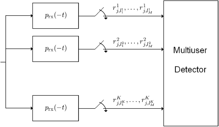
Figure 1: The general structure of the receiver, where $p_{\rm{rx}}(t)$ denotes the received UWB pulse.

and the samples from user $k$ can be expressed as $\tilde{{\bf r}}_{k}=[\tilde{r}_{1}^{k}\cdots\tilde{r}_{N_{f}P}^{k}]$. The proposed receiver is depicted in Figure 1. It is easy to verify that $r_{j,m}^{k}$ is the $((j-1)N_{c}+c_{j}^{k}+l_{m}^{k})$th element of ${\bf r}$ defined in (2), and therefore a matrix, ${\bf G}_{k}$, which performs selection and MRC of selected samples, can be designed such that $\tilde{{\bf r}}_{k}={\bf G}_{k}{\bf r}$.

Based on the samples obtained as in (3), the pulse-symbol detector performs an iterative estimation of users’ symbols. In general, iterative algorithms provide low complexity and close-to-optimal solutions for many problems (see, [15, 23, 31], [6], [18], among many others; a review is found in [24]). The main property of the problems that can be solved efficiently by iterative techniques is that these problems have a very special structure, which allows productive use of iterative procedures. Consider as an example the problem of joint multiuser detection and decoding of error correcting codes in CDMA systems [23]. In this problem, one can employ any multiuser detection algorithm (or more precisely a multiuser receiver [28]) that results in soft decision statistics about every channel symbol. These soft decisions can be fed into any soft decoding algorithm, and the result will be the estimated information symbol. Turbo based algorithms provide an efficient way of iterating between the results obtained by the two constituent algorithms, where each one of these algorithms is designed to solve one part of the problem. Although no such structure exists in the problem of multiuser detection of TH-IR signals, some of the a priori information can be neglected in order to impose a structure suitable for an iterative decoding algorithm. In other words, the spreading operation is regarded as a simple error correcting encoding to facilitate iterative solutions. In this light, TH-IR signaling can be considered as a concatenated coding system, where the inner code involves the modulation of a UWB pulse, and the outer code is a repetition code. This structure is similar to BICM, for which modulation and channel coding comprise the inner and outer codes, respectively [2], [6].

Consideration of TH-IR systems as BICM systems facilitates the design of the pulse-symbol iterative detector, which is composed of two stages [9]. The first stage is denoted as the “pulse detector”, while the second stage is denoted as the “symbol detector”, and the detector iterates between these stages. In the first stage, it is assumed that different pulses from the same user correspond to independent information symbols, while in the second stage the information that several pulses from the same user correspond to the same information symbols is exploited. The second stage acts effectively as a decoder.

III-A The Pulse Detector

Denote by $b_{j}^{k}$ the information symbol carried by the $j$th pulse of the $k$th user. Note that although we know a priori that $b_{(i-1)N_{f}+1}^{k}=\cdots=b_{iN_{f}}^{k}$ for every $k=1,\ldots,K$ and $i=1,\ldots,P$, this information will be ignored by the pulse detector. As such, at the $n$th iteration the pulse detector computes the a posteriori log-likelihood ratio (LLR) of $b_{j}^{k}$, given $\tilde{r}_{j}^{k}$ in (3), the information about the transmitted pulses from other users and the a priori information about $b_{j}^{k}$ provided by the symbol detector, as

$$L_{1}^{n}(b_{j}^{k})\stackrel{{\scriptstyle\triangle}}{{=}}\log\frac{{\rm Pr}(b_{j}^{k}=1|\tilde{r}_{j}^{k})}{{\rm Pr}\left(b_{j}^{k}=-1|\tilde{r}_{j}^{k}\right)}=\log\frac{f\left(\tilde{r}_{j}^{k}|b_{j}^{k}=1\right)}{f\left(\tilde{r}_{j}^{k}|b_{j}^{k}=-1\right)}+\log\frac{{\rm Pr}\left(b_{j}^{k}=1\right)}{{\rm Pr}\left(b_{j}^{k}=-1\right)},$$ (4)

for $j=1,\ldots,PN_{f}$ and $k=1,\ldots,K$, where $f\left(\tilde{r}_{j}^{k}|b_{j}^{k}=i\right)$ is the likelihood of the $j$th combined sample corresponding to the $k$th user given that the transmitted symbol was $i\in\pm 1$. It is seen that the a posteriori LLR is the sum of the a priori LLR of the transmitted symbol, $\log\frac{{\rm Pr}\left(b_{j}^{k}=1\right)}{{\rm Pr}\left(b_{j}^{k}=-1\right)}\stackrel{{\scriptstyle\triangle}}{{=}}\lambda_{2}^{n-1}(b_{j}^{k})$, and the extrinsic information provided by the pulse detector about the transmitted symbol, $\log\frac{f\left(\tilde{r}_{j}^{k}|b_{j}^{k}=1\right)}{f\left(\tilde{r}_{j}^{k}|b_{j}^{k}=-1\right)}\stackrel{{\scriptstyle\triangle}}{{=}}\lambda_{1}^{n}(b_{j}^{k})$ [9].

We first consider the computation of $\log f\left(\tilde{r}_{j}^{k}|b_{j}^{k}\right)$ in (4). From (2), it is easy to deduce the following model for $r_{j,m}^{k}$, which is the received sample from the $m$th path of the $k$th user’s signal in the $j$th frame:

$$r_{j,m}^{k}=[{\bf H}]_{l(j,k,m):}{\bf S}{\bf b}+n_{l(j,k,m)}=\sum_{\tilde{q}=1}^{K}\sum_{\tilde{a}=0}^{N_{f}P-1}b_{\lfloor{\tilde{a}}/N_{f}\rfloor}^{\tilde{q}}[{\bf S}_{\tilde{q}}]_{{\tilde{a}}N_{c}+c_{\tilde{a}}^{\tilde{q}},\lfloor{\tilde{a}}/N_{f}\rfloor}h_{l(j,k,m)-{\tilde{a}}N_{c}-c_{\tilde{a}}^{\tilde{q}}}^{\tilde{q}}+n_{l(j,k,m)},$$ (5)

where $l(j,k,m)$ is the arrival time of the $j$th pulse of the $k$th user via the $m$th path, that is $l(j,k,m)=(j-1)N_{c}+c_{j}^{k}+l_{m}^{k}$; $[{\bf H}]_{l(j,k,m):}$ is the $l(j,k,m)$th row of ${\bf H}$; $[{\bf S}_{m}]_{k,l}$ is the $(k,l)$th element of the matrix ${\bf S}_{m}$; and $n_{l(j,k,m)}$ is the $l(j,k,m)$th element of the noise vector, ${\bf n}$. This model can be simplified further by noting that the vast majority of the summands in (5) are zero. Let ${\mathcal{A}}$ denote the set of distinctive $({\tilde{q}},{\tilde{a}})$ pairs in the right-hand-side (RHS) of (5) such that the corresponding element in the double sum is not zero; i.e.,

$${\mathcal{A}}=\{(\tilde{q},\tilde{a})\in{\mathcal{K}}\times{\mathcal{F}}\,\,|\,\,\,[{\bf S}_{\tilde{q}}]_{{\tilde{a}}N_{c}+c_{\tilde{a}}^{\tilde{q}},\lfloor{\tilde{a}}/N_{f}\rfloor}h_{l(j,k,m)-{\tilde{a}}N_{c}-c_{\tilde{a}}^{\tilde{q}}}^{\tilde{q}}\neq 0\},$$ (6)

where ${\mathcal{K}}=\{1,\ldots,K\}$ and ${\mathcal{F}}=\{0,\ldots,PN_{f}-1\}$. If $K_{j,m}^{k}$ represents the number of summands in (5) that are different from zero, ${\mathcal{A}}$ consists of $K_{j,m}^{k}$ pairs. Note that the pair $(k,j)$ is always in ${\mathcal{A}}$; hence, $K_{j,m}^{k}\geq 1$ for every $j$, $k$ and $m$. Assume, without loss of generality, that the pair $(k,j)$ is the first element of the set ${\mathcal{A}}$.

Let $q(i)$ and $a(i)$ represent, respectively, the first and the second components of the $i$th pair in set ${\mathcal{A}}$ for $i=1,\ldots,K_{j,m}^{k}$. Then, (5) can be further simplified as follows:

$$r_{j,m}^{k}=h_{l_{m}^{k}}^{k}b_{j}^{k}[{\bf S}_{k}]_{jN_{c}+c_{j}^{k},\lfloor j/N_{f}\rfloor}+\tilde{{\bf h}}_{j,m}^{k}\tilde{{\bf b}}_{j,m}^{k}+n_{l(j,k,m)},$$ (7)

where $\tilde{{\bf h}}_{j,m}^{k}=\Bigg{[}\left[{\bf S}_{q(2)}\right]_{a(2)N_{c}+c_{a(2)}^{q(2)},\lfloor a(2)/N_{f}\rfloor}h_{l(j,k,m)-a(2)N_{c}-c_{a(2)}^{q(2)}}^{q(2)},\\ \ldots\left.,\left[{\bf S}_{q\left(K_{j,m}^{k}\right)}\right]_{a\left(K_{j,m}^{k}\right)N_{c}+c_{a\left(K_{j,m}^{k}\right)}^{q\left(K_{j,m}^{k}\right)},\lfloor a\left(K_{j,m}^{k}\right)/N_{f}\rfloor}h_{l(j,k,m)-a\left(K_{j,m}^{k}\right)N_{c}-c_{a\left(K_{j,m}^{k}\right)}^{q\left(K_{j,m}^{k}\right)}}^{q\left(K_{j,m}^{k}\right)}\right]$ and $\tilde{{\bf b}}_{j,m}^{k}=\left[b_{a(2)}^{q(2)},\ldots,b_{a(K_{j,m}^{K})}^{q(K_{j,m}^{k})}\right]^{T}$.

From (3) and (7), $\tilde{r}_{j}^{k}$ can be expressed as

$$\tilde{r}_{j}^{k}=A\,b_{j}^{k}+\sum_{m=1}^{M}h_{l_{m}^{k}}^{k}\tilde{{\bf h}}_{j,m}^{k}\tilde{{\bf b}}_{j,m}^{k}+\tilde{n}_{j}^{k},$$ (8)

where $A=[{\bf S}_{k}]_{jN_{c}+c_{j}^{k},\lfloor j/N_{f}\rfloor}\sum_{m=1}^{M}\left(h_{l_{m}^{k}}^{k}\right)^{2}$, and $\tilde{n}_{j}^{k}=\sum_{m=1}^{M}h_{l_{m}^{k}}^{k}n_{l(j,k,m)}$, which is distributed as ${\mathcal{N}}\left(0\,,\,\tilde{\sigma}^{2}\right)$ with $\tilde{\sigma}^{2}=\sigma_{n}^{2}\sum_{m=1}^{M}\left(h_{l_{m}^{k}}^{k}\right)^{2}$.

Based on (8), the log-likelihood of $\tilde{r}_{j}^{k}$ given $b_{j}^{k}$ is,

$$\log f\left(\tilde{r}_{j}^{k}|b_{j}^{k}\right)=C+\log\sum_{\check{{\bf b}}\in\{\pm 1\}^{\tilde{K}_{j}^{k}}}\exp\left\{-\frac{1}{2\tilde{\sigma}^{2}}\left(\tilde{r}_{j}^{k}-A\,b_{j}^{k}-\sum_{m=1}^{M}h_{l_{m}^{k}}^{k}\tilde{{\bf h}}_{j,m}^{k}\tilde{{\bf b}}_{j,m}\right)^{2}\right\}{\rm Pr}(\check{{\bf b}}),$$ (9)

where $C$ is a constant independent of $j$ and $k$, $\check{{\bf b}}$ is a vector comprised of the distinct $b_{n}^{l}$’s in $\tilde{{\bf b}}_{j,1}^{k},\ldots,\tilde{{\bf b}}_{j,M}^{k}$, and $\tilde{K}_{j}^{k}$ is the size of $\check{{\bf b}}$. Note that $\tilde{K}_{j}^{k}$ represents the total number of pulses that have at least one multipath component arriving at the receiver at the same time as one of the sampled signal paths originating from the $j$th pulse of the $k$th user. Also note that for a given value of $\check{{\bf b}}$, $\tilde{{\bf b}}_{j,m}^{k}$ in (9) is uniquely defined, and ${\rm Pr}(\check{{\bf b}})$ is the a priori probability, which is obtained from the extrinsic information provided by the symbol detector. Since the extrinsic information from the symbol detector is the following LLR, $\lambda_{2}^{n-1}\left(b_{i}^{l}\right)=\log\frac{{\rm Pr}\left(b_{i}^{l}=1\right)}{{\rm Pr}\left(b_{i}^{l}=-1\right)}$ [cf. (12)], it can be shown, with the aid of some algebraic manipulations, that [9]

$${\rm Pr}(\check{{\bf b}})=\frac{1}{2^{\tilde{K}_{j}^{k}}}\prod_{i=1}^{\tilde{K}_{j}^{k}}\left[1+[\check{{\bf b}}]_{i}\tanh\left(\frac{1}{2}\lambda_{2}^{n-1}\left([\check{{\bf b}}]_{i}\right)\right)\right].$$ (10)

From (9) and (10), the a priori LLR of $b_{j}^{k}$ can be written as follows:

$$\log\frac{f\left(\tilde{r}_{j}^{k}|b_{j}^{k}=1\right)}{f\left(\tilde{r}_{j}^{k}|b_{j}^{k}=-1\right)}\stackrel{{\scriptstyle\triangle}}{{=}}\lambda_{1}^{n}\left(b_{j}^{k}\right)$$

$$=\log\frac{\sum_{\check{{\bf b}}\in\{\pm 1\}^{\tilde{K}_{j}^{k}}}e^{-\frac{1}{2\tilde{\sigma}^{2}}\left(\tilde{r}_{j}^{k}-A-\sum_{m=1}^{M}h_{l_{m}^{k}}^{k}\tilde{{\bf h}}_{j,m}^{k}\tilde{{\bf b}}_{j,m}^{k}\right)^{2}}\prod_{i=1}^{\tilde{K}_{j}^{k}}\left[1+[\check{{\bf b}}]_{i}\tanh\left(\frac{1}{2}\lambda_{2}^{n-1}\left([\check{{\bf b}}]_{i}\right)\right)\right]}{\sum_{\check{{\bf b}}\in\{\pm 1\}^{\tilde{K}_{j}^{k}}}e^{-\frac{1}{2\tilde{\sigma}^{2}}\left(\tilde{r}_{j}^{k}+A-\sum_{m=1}^{M}h_{l_{m}^{k}}^{k}\tilde{{\bf h}}_{j,m}^{k}\tilde{{\bf b}}_{j,m}^{k}\right)^{2}}\prod_{i=1}^{\tilde{K}_{j}^{k}}\left[1+[\check{{\bf b}}]_{i}\tanh\left(\frac{1}{2}\lambda_{2}^{n-1}\left([\check{{\bf b}}]_{i}\right)\right)\right]}.$$ (11)

From (11) and (4), it is observed that the a posteriori LLR is given by the sum of the prior information obtained from the symbol detector and the extrinsic information.

III-B The Symbol Detector

The symbol detector exploits the fact that $b_{(i-1)N_{f}+1}^{k}=\cdots=b_{iN_{f}}^{k}$ for every $k=1,\ldots,K$ and $i=1,\ldots,P$. Therefore, the symbol detector computes the a posteriori LLR of $b_{j}^{k}$ given the extrinsic information from the pulse detector, and given $b_{(i-1)N_{f}+1}^{k}=\cdots=b_{iN_{f}}^{k}$ for every $k=1,\ldots,K$ and $i=1,\ldots,P$. It can be shown that this LLR has the following general structure [9]:

$$L_{2}^{n}(b_{j}^{k})\stackrel{{\scriptstyle\triangle}}{{=}}\log\frac{{\rm Pr}\left(b_{j}^{k}=1|\{\lambda_{1}^{n}(b_{j}^{k})\}_{j=1,k=1}^{PN_{f},K};\mbox{constraints on pulses}\right)}{{\rm Pr}\left(b_{j}^{k}=-1|\{\lambda_{1}^{n}(b_{j}^{k})\}_{j=1,k=1}^{PN_{f},K};\mbox{constraints on pulses}\right)}=\underbrace{\sum_{i=N_{f}\lfloor(j-1)/N_{f}\rfloor+1,i\neq j}^{N_{f}\lfloor(j-1)/N_{f}\rfloor+N_{f}}\lambda_{1}^{n}(b_{i}^{k})}_{\lambda_{2}^{n}(b_{j}^{k})}+\lambda_{1}^{n}(b_{j}^{k}),$$ (12)

where the constraints are $b_{(i-1)N_{f}+1}^{k}=\cdots=b_{iN_{f}}^{k}$ for every $k=1,\ldots,K$ and $i=1,\ldots,P$. In (12), the a posteriori LLR at the output of the symbol detector is expressed as the sum of the prior information from the pulse detector, $\lambda_{1}^{n}(b_{j}^{k})$, and the extrinsic information about $b_{j}^{k}$, denoted by $\lambda_{2}^{n}(b_{j}^{k})$. This extrinsic information is obtained from the information about all the pulses except the $j$th pulse of the $k$th user. In the next iteration this information is fed back to the pulse detector as a priori information about the $j$th pulse of the $k$th user.

Note that the structure of the pulse-symbol detector is similar to the joint-over-antenna turbo receiver in [18], which employs multiple turbo loops for each antenna, by considering “composite” modulation for multiple antennas as the inner code, and channel coding for different users as the outer code. The main differences are that, for the pulse-symbol detector, the outer code is a simple repetition code, while the inner code is a binary phase shift keying modulation, and that there are also TH and polarity randomization operations in the pulse-symbol detector, which randomize the positions and the polarities of the pulses in different frames.

III-C Complexity

It is easily seen that computing $\lambda_{1}\left(b_{j}^{k}\right)$ of (11) is the most complex task in the pulse-symbol detector. The complexity of computing $\lambda_{1}\left(b_{j}^{k}\right)$ is exponential in the total number $\tilde{K}_{j}^{k}$ of pulses that have at least one multipath component arriving at the receiver at the same time as one of the sampled signal paths originating from the $j$th pulse of the $k$th user. That is, as can be observed from (11), the complexity of computing $\lambda_{1}\left(b_{j}^{k}\right)$ is ${\mathcal{O}}\left(2^{\tilde{K}_{j}^{k}}\right)$. Since there are $N_{f}$ pulses per symbol per user, the complexity of one iteration per symbol per user is easily seen to be ${\mathcal{O}}\left(\sum_{j=1}^{N_{f}}2^{\tilde{K}_{j}^{k}}\right)={\mathcal{O}}\left(2^{Y(K)}\right)$, where $Y(K)\stackrel{{\scriptstyle\triangle}}{{=}}\max_{j=1,\ldots,N_{f}}\tilde{K}_{j}^{k}$. Denoting by $N_{\rm{i}}$ the number of iterations made by the pulse-symbol detector, the complexity of the pulse-symbol detector is ${\mathcal{O}}\left(N_{\rm{i}}2^{Y(K)}\right)$ per symbol per user.

$\tilde{K}_{j}^{k}$ is a random variable depending on the channel impulse response, the TH sequence, and the number of users in the system. It is hard to compare the complexity of the pulse-symbol detector, which is random, with the complexity of multiuser detection algorithms that have fixed complexity, e.g., the optimal detector. Nevertheless, if, for example, the probability of the event $N_{\rm{i}}2^{Y(K)}>2^{K}$ is very low, then, roughly speaking, the proposed algorithm is simpler than the optimal detector.

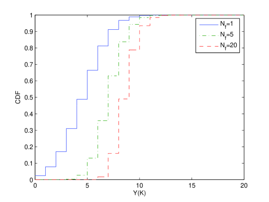
Figure 2: CDF of $\max_{j=1,\ldots,N_{f}}\tilde{K}_{j}^{k}$ for various pulse rates.

The exact distribution of $Y(K)$ is very complicated, and moreover, this distribution depends on the exact channel structure, the number of paths arriving at the receiver, and the TH sequences. In what follows, numerical examples are used to demonstrate the complexity of the pulse-symbol detector. In particular, consider a system with $20$ users, each transmitting at rate of $2$ MBits/sec over a $0.5$ GHz UWB indoor channel [7]. The receiver is sampling the first $10$ multipath components; i.e., ${\mathcal{L}}=\{1,2,\ldots,10\}$. Figure 2 depicts the empirical cumulative distribution function (CDF) of $Y(K)$, averaged over $100$ different channel realizations from the channel model $1$ (CM-1) of the IEEE 802.15.3a channel model, for systems transmitting one, five and twenty pulses per symbols ($N_{f}=1,5,20$). It is clear that the complexity of the pulse-symbol detector decreases as the pulse rate, $N_{f}$, decreases. This is expected because, as the pulse rate decreases, the probability of collisions decreases as well, which reduces the complexity of the pulse-symbol detector. Nevertheless, the complexity of the pulse-symbol detector can be large even for moderate numbers of pulses per symbol. In the next section, two low-complexity implementations are presented.

IV Low Complexity Implementations

The complexity of the pulse-symbol detector varies considerably with the system pulse rate, $N_{f}$. An increase in the pulse rate increases the algorithm complexity, and this complexity can be large even for moderate pulse rates or numbers of users. In what follows two low complexity implementations are described. The first one is based on approximating part of the multiple access interference (MAI) by a Gaussian random variable, while the second one is based on soft interference cancellation.

IV-A Low-Complexity Implementation: The Gaussian Approximation Approach

The high complexity of the pulse-symbol detector is due solely to the pulse detector where the a priori LLR of a received sample given the transmitted symbol, $\lambda_{1}(b_{j}^{k})$, is computed. In recent studies (see, [3, 29, 34, 7], and references therein), UWB channels are commonly characterized as multipath channels with large numbers of paths, and delay spreads of up to a few tens of nanoseconds. These large delay spreads are equivalent to discrete-time channels having more than one hundred taps. Although the UWB channel consists of many taps, most of them are weak compared with the strongest tap, and only about five to ten taps are weaker by no more than $10$ dB than the strongest tap. Therefore, most of the pulses colliding with the pulse of interest arrive via weak paths.

In order to reduce the complexity of the pulse-symbol detector, we propose to model the MAI resulting from the pulses arriving via weak paths by a Gaussian random variable. Recall that $h_{l_{m}^{k}}^{k}$ is the gain of the $m$th path, through which the pulse of interest arrives at the receiver. In order to reduce the complexity of computing $\lambda_{1}^{n}\left(b_{j}^{k}\right)$, the receiver sets a threshold $T$ (in dB) and all the pulses colliding with the pulse of interest are divided into two groups. The first group contains all the pulses that collide with the pulse of interest and that arrive via paths that are weaker than the $m$th path of user $k$ by no more than $T$ dB (i.e., each path has an amplitude of at least $10\log_{10}\left|h_{l_{m}^{k}}^{k}\right|-T$ dB). The second group contains all the pulses that collide with the pulse of interest and that arrive via paths that are weaker than $h_{l_{m}^{k}}^{k}$ by more than $T$ dB. Denote by $I_{j,m}^{k}$ and $\bar{I}_{j,m}^{k}$ the indices of the pulses belonging to the first and second group, respectively; that is,

$$I_{j,m}^{k}=\left\{i\,\Big{|}\,10\log_{10}\left|h_{l_{m}^{k}}^{k}\right|-10\log_{10}\left|h_{l(j,k,m)-a(i)N_{c}-c_{a(i)}^{q(i)}}^{q(i)}\right|\leq T,i=2,\ldots,K_{j,m}^{k}\right\},$$ (13)

and similarly define $\bar{I}_{j,m}^{k}$.

A model for $r_{j,m}^{k}$ can be written in terms of $I_{j,m}^{k}$ and $\bar{I}_{j,m}^{k}$ as follows:

$$r_{j,m}^{k} =h^{k}_{l_{m}^{k}}b_{j}^{k}[{\bf S}_{k}]_{jN_{c}+c_{j}^{k},\lfloor j/N_{f}\rfloor}+\sum_{i\in I_{j,m}^{k}}b_{a(i)}^{q(i)}\left[{\bf S}_{q(i)}\right]_{a(i)N_{c}+c_{a(i)}^{q(i)},\lfloor a(i)/N_{f}\rfloor}h_{l(j,k,m)-a(i)N_{c}-c_{a(i)}^{q(i)}}^{q(i)}$$

$$+\sum_{i\in\bar{I}_{j,m}^{k}}b_{a(i)}^{q(i)}\left[{\bf S}_{q(i)}\right]_{a(i)N_{c}+c_{a(i)}^{q(i)},\lfloor a(i)/N_{f}\rfloor}h_{l(j,k,m)-a(i)N_{c}-c_{a(i)}^{q(i)}}^{q(i)}+n_{l(j,k,m)},$$ (14)

where the first term on the RHS represents the part of the received signal resulting from the pulse of interest, the second term on the RHS represents that part of the MAI resulting from strong interference, the third term on the RHS represents that part of the MAI resulting from weak interference, and the fourth term on the RHS represents the additive Gaussian noise. Since most of the paths are considerably weaker than the main path, it is expected that $|\bar{I}_{j,m}^{k}|>>|I_{j,m}^{k}|$. As such, the third term on the RHS of (14) is the sum of a large number of random variables and we propose to model this sum as a Gaussian random variable. The mean and the variance of the third term on the RHS of (14) are zero and $\sum_{i\in\bar{I}_{j,m}^{k}}\left|h_{l(j,k,m)-a(i)N_{c}-c_{a(i)}^{q(i)}}^{q(i)}\right|^{2}$, respectively. Thus we use the following approximation:

$$\sum_{i\in\bar{I}_{j,m}^{k}}b_{a(i)}^{q(i)}\left[{\bf S}_{q(i)}\right]_{a(i)N_{c}+c_{a(i)}^{q(i)},\lfloor a(i)/N_{f}\rfloor}h_{l(j,k,m)-a(i)N_{c}-c_{a(i)}^{q(i)}}^{q(i)}\sim{\mathcal{N}}\left(0,\sum_{i\in\bar{I}_{j,m}^{k}}\left|h_{l(j,k,m)-a(i)N_{c}-c_{a(i)}^{q(i)}}^{q(i)}\right|^{2}\right).$$ (15)

Approximating the part of the MAI corresponding to weak pulses colliding with the pulse of interest by a Gaussian random variable results in the following approximate model for $r_{j,m}^{k}$:

$$r_{j,m}^{k} \approx h^{k}_{l_{m}^{k}}b_{j}^{k}[{\bf S}_{k}]_{jN_{c}+c_{j}^{k},\lfloor j/N_{f}\rfloor}+\sum_{i\in I_{j,m}^{k}}b_{a(i)}^{q(i)}\left[{\bf S}_{q(i)}\right]_{a(i)N_{c}+c_{a(i)}^{q(i)},\lfloor a(i)/N_{f}\rfloor}h_{l(j,k,m)-a(i)N_{c}-c_{a(i)}^{q(i)}}^{q(i)}+\check{n}_{j,m}^{k}$$

$$=h^{k}_{l_{m}^{k}}b_{j}^{k}[{\bf S}_{k}]_{jN_{c}+c_{j}^{k},\lfloor j/N_{f}\rfloor}+\tilde{\tilde{{\bf h}}}_{j,m}^{k}\tilde{\tilde{{\bf b}}}_{j,m}^{k}+\check{n}_{j,m}^{k},$$ (16)

where $\check{n}_{j,m}^{k}$ is a zero mean Gaussian random variable with variance $(\sigma_{j,m}^{k})^{2}=\sigma_{n}^{2}+\sum_{i\in\bar{I}_{j,m}^{k}}\left|h_{l(j,k,m)-a(i)N_{c}-c_{a(i)}^{q(i)}}^{q(i)}\right|^{2}$; $\tilde{\tilde{{\bf h}}}_{j,m}^{k}=\left[\left[{\bf S}_{q(I_{1})}\right]_{a(I_{1})N_{c}+c_{a(I_{1})}^{q(I_{1})},\lfloor a(I_{1})/N_{f}\rfloor}h_{l(j,k,m)-a(I_{1})N_{c}-c_{a(I_{1})}^{q(I_{1})}}^{q(I_{1})},\right.\\ \ldots\left.,\left[{\bf S}_{q\left(I_{|I|}\right)}\right]_{a\left(I_{|I|}\right)N_{c}+c_{a\left(I_{|I|}\right)}^{q\left(I_{|I|}\right)},\lfloor a\left(I_{|I|}\right)/N_{f}\rfloor}h_{l(j,k,m)-a\left(I_{|I|}\right)N_{c}-c_{a\left(I_{|I|}\right)}^{q\left(I_{|I|}\right)}}^{q\left(I_{|I|}\right)}\right]$ and $\tilde{\tilde{{\bf b}}}_{j,m}^{k}=\left[b_{a(I_{1})}^{q(I_{1})},\ldots,b_{a(I_{|I|})}^{q(I_{|I|})}\right]$. Using the same derivations leading to (11) and (16), the a priori log-likelihood ratio of $\tilde{r}_{j}^{k}=\sum_{m=1}^{M}h_{l_{m}^{k}}^{k}r_{j,m}^{k}$ given $b_{j}^{k}$ is then approximated by,

$$\tilde{\lambda}_{1}^{n}\left(b_{j}^{k}\right)=\log\frac{f\left(\tilde{r}_{j}^{k}|b_{j}^{k}=1\right)}{f\left(\tilde{r}_{j}^{k}|b_{j}^{k}=-1\right)}\cong$$ (17)

$$\log\frac{\sum_{\check{\check{{\bf b}}}\in\{\pm 1\}^{\tilde{\tilde{K}}_{j}^{k}}}e^{-\frac{1}{2\tilde{\tilde{\sigma}}^{2}}\left(\tilde{r}_{j}^{k}-\tilde{A}-\sum_{m=1}^{M}h_{l_{m}^{k}}^{k}\tilde{\tilde{{\bf h}}}_{j,m}^{k}\tilde{\tilde{{\bf b}}}_{j,m}^{k}\right)^{2}}\prod_{i=1}^{\tilde{\tilde{K}}_{j}^{k}}\left[1+[\check{\check{{\bf b}}}]_{i}\tanh\left(\frac{1}{2}\lambda_{2}^{n-1}\left([\check{\check{{\bf b}}}]_{i}\right)\right)\right]}{\sum_{\check{\check{{\bf b}}}\in\{\pm 1\}^{\tilde{\tilde{K}}_{j}^{k}}}e^{-\frac{1}{2\tilde{\tilde{\sigma}}^{2}}\left(\tilde{r}_{j}^{k}+\tilde{A}-\sum_{m=1}^{M}h_{l_{m}^{k}}^{k}\tilde{\tilde{{\bf h}}}_{j,m}^{k}\tilde{\tilde{{\bf b}}}_{j,m}^{k}\right)^{2}}\prod_{i=1}^{\tilde{\tilde{K}}_{j}^{k}}\left[1+[\check{\check{{\bf b}}}]_{i}\tanh\left(\frac{1}{2}\lambda_{2}^{n-1}\left([\check{\check{{\bf b}}}]_{i}\right)\right)\right]},$$

where $\tilde{A}=[{\bf S}_{k}]_{jN_{c}+c_{j}^{k},\lfloor j/N_{f}\rfloor}\sum_{m=1}^{M}\left(h_{l_{m}^{k}}^{k}\right)^{2}$, $\tilde{\tilde{\sigma}}^{2}$ is the variance of $\sum_{m=1}^{M}h_{l_{m}^{k}}^{k}\check{n}_{j,m}^{k}$, which is $\sum_{m=1}^{M}|h_{l_{m}^{k}}^{k}|^{2}(\sigma_{j,m}^{k})^{2}$, $\check{\check{{\bf b}}}$ is a vector comprised of the distinct $b_{n}^{l}$’s in $\tilde{\tilde{{\bf b}}}_{j,1}^{k},\ldots,\tilde{\tilde{{\bf b}}}_{j,M}^{k}$, and $\tilde{\tilde{K}}_{j}^{k}$ is the size of $\check{\check{{\bf b}}}$.

The proposed low complexity implementation computes the approximate a priori log-likelihood ratios, $\left\{\tilde{\lambda}_{1}^{n}\left(b_{j}^{k}\right)\right\}$, instead of the exact a priori log-likelihood ratios. The symbol detector uses these approximate LLRs as the extrinsic information, and it computes a new set of extrinsic information variables, $\{\lambda_{2}^{n}(b_{j}^{k})\}$, based on the approximate LLRs provided by the pulse detector. The algorithm continues to iterate between the two stages until convergence is reached.

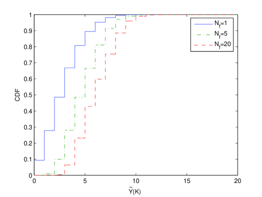
Figure 3: CDF of $\max_{j=1,\ldots,N_{f}}\tilde{\tilde{K}}_{j}^{k}$ for various pulse rates and $T=3$ dB.

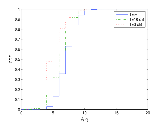
Figure 4: CDF of $\max_{j=1,\ldots,N_{f}}\tilde{\tilde{K}}_{j}^{k}$ for $N_{f}=5$ and various threshold values.

The complexity of the proposed scheme depends on the exact number of strong pulses colliding with the pulse of interest, which is again a random variable. It is easily seen that the complexity of this implementation is ${\mathcal{O}}\left(2^{\tilde{Y}(K)}\right)$, where $\tilde{Y}(K)=\max_{j=1,\ldots,N_{f}}\tilde{\tilde{K}}_{j}^{k}$. Again, we resort to a numerical example in order to demonstrate the complexity of the proposed detector. Consider a system having $20$ users, each transmitting at a rate of $2$ MBits/sec over a $0.5$ GHz UWB indoor channel [7]. The receiver is sampling the first $10$ multipath components; i.e., ${\mathcal{L}}=\{1,2,\ldots,10\}$, and the threshold $T$ is set to $3$ dB. Figure 3 depicts the empirical CDF of $\tilde{Y}(K)$, averaged over $100$ different channel realizations from the channel model $1$ (CM-1) of the IEEE 802.15.3a channel model, for systems transmitting one, five and twenty pulses per symbols ($N_{f}=1,5,20$). By comparing Figure 2 and Figure 3, the reduction in the complexity compared with the complexity of the pulse-symbol detector can be observed. In Figure 4, the empirical CDF is plotted for $N_{f}=5$ and various threshold values. It is observed that as the threshold is decreased, fewer collisions are considered as strong ones, which reduces the complexity of the algorithm.

Using the same approach, there are other ways of reducing the complexity of the pulse-symbol detector. For example, one can divide the received pulses into two groups based on their relative strengths. In this approach, a threshold $\delta$ will be set in advance, and the MAI caused by all but the $\delta$ strongest colliding pulses will be modelled as a Gaussian random variable. In this approach the complexity of the receiver is limited by $N_{f}2^{\delta}$ per symbol per user.

IV-B Low-Complexity Implementation: The Soft Interference Cancellation Approach

The complexity of the low-complexity implementation presented in the previous subsection might still be high for large numbers of users or pulse rates. As such, an even simpler implementation method is required. In what follows a very low complexity implementation based on soft interference cancellation is presented.

Recall that the most complex task in the pulse-symbol detector is the computation of the a priori log-likelihood ratio of the received sample given the transmitted pulse, $\lambda_{1}\left(b_{j}^{k}\right)=\log\frac{f\left(\tilde{r}_{j}^{k}|b_{j}^{k}=1\right)}{f\left(\tilde{r}_{j}^{k}|b_{j}^{k}=-1\right)}$. Our aim is to find a simple way to approximate $\lambda_{1}\left(b_{j}^{k}\right)$, and soft-interference cancellation provides us with such a method [16, 19]. Recall that the model for $\tilde{r}_{j}^{k}$ is given by $\tilde{r}_{j}^{k}=\sum_{m=1}^{M}r_{j,m}^{k}$, where $r_{j,m}^{k}=h_{l_{m}^{k}}^{k}b_{j}^{k}[{\bf S}_{k}]_{jN_{c}+c_{j}^{k},\lfloor j/N_{f}\rfloor}+\tilde{{\bf h}}_{j,m}^{k}\tilde{{\bf b}}_{j,m}^{k}+n_{l(j,k,m)}$. In soft-interference cancellation methods, the first step is to form a soft estimate of $\tilde{{\bf b}}_{j,m}^{k}$. This soft estimate is the conditional mean of $\tilde{{\bf b}}_{j,m}^{k}$ based on our current knowledge. We denote this soft estimate by $\bar{\tilde{{\bf b}}}_{j,m}^{k}={\rm{E}}\left\{\tilde{{\bf b}}_{j,m}^{k}\big{|}\{\lambda_{2}\left(b_{j}^{k}\right)\}\right\}$, which is given by

$$\left[\bar{\tilde{{\bf b}}}_{j,m}^{k}\right]_{i}=\left[{\rm{E}}\left\{\tilde{{\bf b}}_{j,m}^{k}|\{\lambda_{2}\left(b_{j}^{k}\right)\}\right\}\right]_{i}={\rm{E}}\left\{b_{a(i)}^{q(i)}\right\}={\rm Pr}\left(b_{a(i)}^{q(i)}=1\right)-{\rm Pr}\left(b_{a(i)}^{q(i)}=-1\right)$$

$$\quad\quad=\frac{1}{2}\left[1+\tanh\left(\frac{1}{2}\lambda_{2}\left(b_{a(i)}^{q(i)}\right)\right)\right]-\frac{-1}{2}\left[1-\tanh\left(\frac{1}{2}\lambda_{2}\left(b_{a(i)}^{q(i)}\right)\right)\right]=\tanh\left(\frac{1}{2}\lambda_{2}\left(b_{a(i)}^{q(i)}\right)\right).$$ (18)

Assuming that this soft estimate is reliable, the remodulated signal $\tilde{{\bf h}}_{j,m}^{k}\bar{\tilde{{\bf b}}}_{j,m}^{k}$ is subtracted from $r_{j,m}^{k}$ resulting in

$$\bar{r}_{j,m}^{k}\stackrel{{\scriptstyle\triangle}}{{=}}r_{j,m}^{k}-\tilde{{\bf h}}_{j,m}^{k}\bar{\tilde{{\bf b}}}_{j,m}^{k}=h_{l_{m}^{k}}^{k}b_{j}^{k}[{\bf S}_{k}]_{jN_{c}+c_{j}^{k},\lfloor j/N_{f}\rfloor}+\tilde{{\bf h}}_{j,m}^{k}\left(\tilde{{\bf b}}_{j,m}^{k}-\bar{\tilde{{\bf b}}}_{j,m}^{k}\right)+n_{l(j,k,m)}.$$ (19)

Subtracting the remodulated signal from $r_{j,m}^{k}$ results in the reduction of the MAI. Since the number of collisions is large, the remaining MAI, $\tilde{{\bf h}}_{j,m}^{k}\left(\tilde{{\bf b}}_{j,m}^{k}-\bar{\tilde{{\bf b}}}_{j,m}^{k}\right)=\sum_{i=2}^{K_{j,m}^{k}}\left[\tilde{{\bf h}}_{j,m}^{k}\right]_{i}\left(b_{a(i)}^{q(i)}-{\rm{E}}\left\{b_{a(i)}^{q(i)}\right\}\right)$, is approximated by a Gaussian random variable, as follows:

$$\sum_{i=2}^{K_{j,m}^{k}}\left[\tilde{{\bf h}}_{j,m}^{k}\right]_{i}\left(b_{a(i)}^{q(i)}-{\rm{E}}\left\{b_{a(i)}^{q(i)}\right\}\right)\sim{\mathcal{N}}\left(\mu_{j,m}^{k},(\sigma_{j,m}^{k})^{2}\right)$$ (20)

with

$$\mu_{j,m}^{k}={\rm{E}}\left\{\sum_{i=2}^{K_{j,m}^{k}}\left[\tilde{{\bf h}}_{j,m}^{k}\right]_{i}\left(b_{a(i)}^{q(i)}-E\left\{b_{a(i)}^{q(i)}\right\}\tilde{{\bf b}}_{j,m}^{k}\right)\right\}=\sum_{i=2}^{K_{j,m}^{k}}\left[\tilde{{\bf h}}_{j,m}^{k}\right]_{i}{\rm{E}}\left\{\left(b_{a(i)}^{q(i)}-E\left\{b_{a(i)}^{q(i)}\right\}\right)\right\}=0$$ (21)

and

$$(\sigma_{j,m}^{k})^{2} ={\rm{Var}}\left\{\sum_{i=2}^{K_{j,m}^{k}}\left[\tilde{{\bf h}}_{j,m}^{k}\right]_{i}\left(b_{a(i)}^{q(i)}-{\rm{E}}\left\{b_{a(i)}^{q(i)}\right\}\right)\right\}={\rm{E}}\left\{\left(\sum_{i=2}^{K_{j,m}^{k}}\left[\tilde{{\bf h}}_{j,m}^{k}\right]_{i}\left(b_{a(i)}^{q(i)}-{\rm{E}}\left\{b_{a(i)}^{q(i)}\right\}\right)\right)^{2}\right\}$$

$$=\sum_{i=2}^{K_{j,m}^{k}}\left[\tilde{{\bf h}}_{j,m}^{k}\right]_{i}{\rm{Var}}\left\{b_{a(i)}^{q(i)}\right\}=\sum_{i=2}^{K_{j,m}^{k}}\left[\tilde{{\bf h}}_{j,m}^{k}\right]^{2}_{i}\left(1-\left(\left[\tilde{\tilde{b}}_{j}^{k}\right]_{i}\right)^{2}\right),$$ (22)

where ${\rm{E}}\left\{\left(b_{a(i)}^{q(i)}-{\rm{E}}\left\{b_{a(i)}^{q(i)}\right\}\right)\left(b_{a(l)}^{q(l)}-{\rm{E}}\left\{b_{a(l)}^{q(l)}\right\}\right)\right\}=0$ for $i\neq l$, and ${\rm{Var}}\left\{b_{a(i)}^{q(i)}\right\}={\rm{E}}\left\{\left(b_{a(i)}^{q(i)}\right)^{2}\right\}-\left({\rm{E}}\left\{\left(b_{a(i)}^{q(i)}\right)\right\}\right)^{2}=1-\left(\left[\tilde{\tilde{b}}_{j}^{k}\right]_{i}\right)^{2}$ are used.

Then, the soft estimate for $\tilde{r}_{j}^{k}$ can be obtained as

$$\bar{\tilde{r}}_{j}^{k}=\sum_{m=1}^{M}h_{l_{m}^{k}}^{k}\bar{r}_{j,m}^{k}=\tilde{A}\,b_{j}^{k}+\bar{\tilde{n}}_{j}^{k},$$ (23)

where $\tilde{A}=[{\bf S}_{k}]_{jN_{c}+c_{j}^{k},\lfloor j/N_{f}\rfloor}\sum_{m=1}^{M}\left(h_{l_{m}^{k}}^{k}\right)^{2}$, and $\bar{\tilde{n}}_{j}^{k}=\sum_{m=1}^{M}h_{l_{m}^{k}}^{k}\bar{n}_{j,m}^{k}$, with $\bar{n}_{j,m}^{k}=\tilde{{\bf h}}_{j,m}^{k}\left(\tilde{{\bf b}}_{j,m}^{k}-\bar{\tilde{{\bf b}}}_{j,m}^{k}\right)+n_{l(j,k,m)}$.

In the proposed very low-complexity implementation of the pulse-symbol algorithm, the pulse detector computes the a priori log-likelihood ratio of $\bar{\tilde{r}}_{j}^{k}$ given the transmitted symbol, instead of the a priori log-likelihood ratio of $\tilde{r}_{j}^{k}$ given the transmitted symbol. Denote by $\tilde{\tilde{\lambda}}_{1}^{n}\left(b_{j}^{k}\right)$ this log-likelihood ratio; that is, $\tilde{\tilde{\lambda}}_{1}^{n}\left(b_{j}^{k}\right)\stackrel{{\scriptstyle\triangle}}{{=}}\log\frac{f\left(\bar{\tilde{r}}_{j}^{k}|b_{j}^{k}=1\right)}{f\left(\bar{\tilde{r}}_{j}^{k}|b_{j}^{k}=-1\right)}$. By using the Gaussian approximation for the residual MAI as shown in (20), $\tilde{\tilde{\lambda}}_{1}^{n}\left(b_{j}^{k}\right)$ is easily seen to be given by

$$\tilde{\tilde{\lambda}}_{1}^{n}\left(b_{j}^{k}\right)=\frac{-\left(\bar{\tilde{r}}_{j}^{k}-\tilde{A}\right)^{2}+\left(\bar{\tilde{r}}_{j}^{k}+\tilde{A}\right)^{2}}{\sum_{m=1}^{M}\left(h^{k}_{l_{m}^{k}}\right)^{2}\left(\sigma_{n}^{2}+(\sigma_{j,m}^{k})^{2}\right)}=\frac{4\tilde{A}\bar{\tilde{r}}_{j}^{k}}{\sum_{m=1}^{M}\left(h^{k}_{l_{m}^{k}}\right)^{2}\left(\sigma_{n}^{2}+(\sigma_{j,m}^{k})^{2}\right)}.$$ (24)

As in the previously proposed low complexity implementation, the pulse detector computes the a priori log-likelihood ratios, $\left\{\tilde{\tilde{\lambda}}_{1}^{n}\left(b_{j}^{k}\right)\right\}$, instead of the exact a priori log-likelihood ratios. The symbol detector uses these approximated LLRs as its extrinsic information, and it computes a new set of extrinsic information, $\{\lambda_{2}^{n}(b_{j}^{k})\}$, based on the approximated LLRs provided by the pulse detector. The algorithm then continues to iterate between the two stages until convergence is reached.

V Simulations

In this section, simulation results are presented in order to investigate the performance of various receiver structures as a function of the signal-to-noise ratio (SNR). The UWB indoor channel model reported by the IEEE 802.15.3a task group is used for generating UWB multipath channels [7], and the uplink of a synchronous TH-IR system with $N_{f}=5$, $N_{c}=250$, and a bandwidth of $0.5$ GHz is considered. It is assumed that there is no inter-frame interference (IFI) in the system. Note, however, that the analysis in Section III and IV cover scenarios with IFI, as well.

In Figure 5, bit error rates (BERs) of various receivers are plotted as functions of the SNR using $100$ realizations of CM-1 [7]. There are $5$ users in the environment ($K=5$), where the first user is assumed to be the user of interest. Each interfering user is modeled to have $10$ dB more power than the user of interest so that an MAI-limited scenario can be investigated. Note that the benefits of iterative multiuser detectors become more obvious in the MAI-limited regime. At all the receivers, the first $25$ multipath components are employed; i.e., ${{\mathcal{L}}}^{1}=\{1,\ldots,25\}$. In the figure, the curve labeled “MRC-Rake” corresponds to the performance of a conventional MRC-Rake receiver [4]; the curves labeled “LC” correspond to the performance of the low complexity implementation method based on the Gaussian approximation ($T=10$ dB is used); and the curves labeled “SIC” correspond to the performance of the low complexity implementation method based on soft interference cancellation. Also, the single user bound is plotted for an MRC-Rake receiver in the absence of interfering users. From the figure, it is observed that the BERs of the proposed detectors are considerably lower than those of the MRC-Rake. In addition, after two iterations, the performance of the proposed receivers gets very close to that of a single user system. Finally, the low complexity implementation based on the Gaussian approximation out-performs the low complexity implementation based on soft interference cancellation on the first iteration, which is a price paid for the lower complexity of the latter algorithm. In other words, the soft interference approach estimates the overall MAI by first order moments, and approximates the difference between the MAI and the MAI estimate by Gaussian random variables, which reduces the complexity significantly but also causes a performance loss due to a more extensive Gaussian approximation compared to the low complexity implementation that uses Gaussian approximations only for weak MAI terms. However, after two iterations, both receivers get very close to the single-user bound, and the low complexity implementation based on soft interference cancellation becomes more advantageous due to its lower computation complexity (cf. Figure 7).

In Figure 6, the same parameters as in the previous case are used, and performance of the low complexity implementation based on the Gaussian approximation is investigated for various threshold values. As can be observed from the plot, as the threshold is decreased; i.e., as more MAI terms are approximated by Gaussian random variables, the performance of the algorithm degrades. In other words, there is a tradeoff between performance and complexity as expected from the study in Section IV-A. Also note that since each interfering user is $10$ dB stronger than the user of interest, there is not much difference between the $T=10$ dB and $T=0$ dB cases (as most of the significant MAI terms are usually above the threshold in both cases), whereas the performance degrades significantly for the $T=-10$ dB case.

Next, the performance of the receivers is investigated for CM-3 of the IEEE 802.15.3a channel model, where $T=0$ dB is used for the low complexity implementation based on the Gaussian approximation. The same observations as in Figure 5 are made. The main difference in this case is the increase in the BERs, which is a result of the larger channel delay spread of the channel model used in the simulations. In other words, less energy is collected on the average, which results in an increase in average BERs.

In order to compare the performance of the proposed receivers under computational constraints, the performance loss (in dB) of each receiver compared to a single user receiver is plotted versus the average number of multiplication operations per user in Figure 7. The performance loss is calculated as the difference between the SNR needed for the receiver to achieve a BER of $10^{-3}$ and the SNR of the single user receiver at BER=$10^{-3}$. For each receiver, the points on the curve are obtained for $1$, $2$ and $3$ iterations. From Figure 7, it is concluded that the low complexity implementation based on soft interference cancellation provides a better performance-complexity tradeoff than the low complexity implementation based on the Gaussian approximation.

Finally, the performance of the receivers that are sampling only the first $5$ multipath components (i.e., ${{\mathcal{L}}}^{1}=\{1,2,3,4,5\}$) is investigated. In this case, it is observed from Figure 8 that the proposed receivers can still perform very closely to the single-user bound, whereas the MRC-Rake receiver experiences a serious error floor.

VI Summary and Concluding Remarks

In this paper an iterative approach, the pulse-symbol detector, for multiuser detection in TH-IR systems has been presented for frequency-selective environments. In this approach, the detection problem is divided, artificially, into two parts, and the proposed algorithm iterates between these two parts. In each iteration, the algorithm passes extrinsic information between the two parts, resulting in an increase in the accuracy of the decisions made by the detector. The complexity of the proposed detector is random; hence, comparing the complexity of this detector with other fixed complexity algorithms is complicated. Nevertheless, we have demonstrated, via simulations, that there are scenarios were the complexity of the proposed detector is lower than the complexity of the optimal detector, while in others it is higher.

In addition, two low-complexity implementations have been presented. The first implementation is based on approximating parts of the MAI by a Gaussian random variable and the second is based on soft interference cancellation. The complexity of both implementations is quite low, and we believe that these algorithms could be used in practical systems. The performance characteristics of these low-complexity implementations have been examined using simulations. We have shown that these algorithms typically get very close to the single-user bound after only a few iterations, and outperform the MRC-Rake substantially.

The proposed multiuser detection algorithms were described under the assumption of synchronous users. However, it is easily seen that this assumption was made only for notational simplicity. The pulse detector inherently ignores any information about the symbols and their structure, and in particular their timing. It uses only the information about the individual pulses that collide with the pulse of interest. The symbol detector uses the results of the pulse detector for pulses that correspond to the symbol of interest. As such, the symbol detector is independent of the other symbols from the same user or from the symbols from other users. In summary, it is evident that synchronization among users is not required. Moreover, it is easy to design a serialized version of the proposed algorithm in the sense that the receiver process on-the-fly new samples at the expense of performance degradation. In summary, the only requirement from the receiver is the knowledge of each user’s symbol timing, which is commonly obtained during synchronization phases in practical systems.

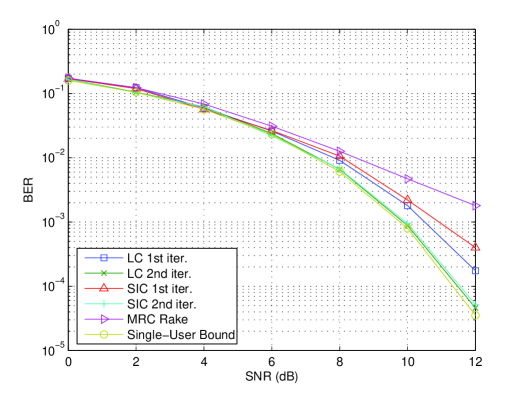
Figure 5: BER as a function of the SNR for various receivers.

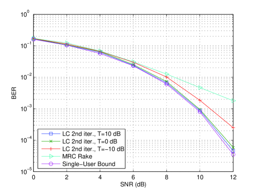
Figure 6: BER as a function of the SNR for various receivers, where the Gaussian approximation technique is plotted for various threshold values.

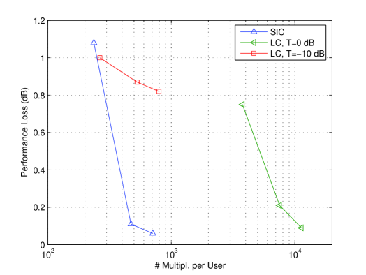
Figure 7: The distance in dB from a single user system at BER=$10^{-3}$ versus the average number of multiplication operations per user. For each receiver, the points are obtained for $1$, $2$ and $3$ iterations (${{\mathcal{L}}}^{1}=\{1,\ldots,10\}$).

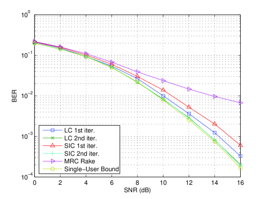
Figure 8: BER as a function of the SNR for various receivers.

References

- [1] S. Buzzi and H. V. Poor. Channel estimation and multiuser detection in long-code DS/CDMA systems. IEEE Journal on Selected Areas in Communications, 19(8):1476–1487, Aug. 2001.
- [2] G. Caire, G. Taricco, and E. Biglieri. Bit-interleaved coded modulation. IEEE Transactions on Information Theory, 44(3):927 –946, May 1998.
- [3] D. Cassioli, M. Z. Win, and A. F. Molisch. The ultra-wide bandwidth indoor channel: From statistical model to simulations. IEEE Journal on Selected Areas in Communications, 20(6):1247–1257, Aug. 2002.
- [4] D. Cassioli, M. Z. Win, F. Vatalaro, and A. F. Molisch. Performance of low-complexity RAKE reception in a realistic UWB channel. In Proc. IEEE International Conference on Communications (ICC 2002), volume 2, pages 763–767, New York City, NY, April 28-May 2 2002.
- [5] J. D. Choi and W. E. Stark. Performance of ultra-wideband communications with suboptimal receivers in multipath channels. IEEE Journal on Selected Areas in Communications, 20(9):1754–1767, Dec. 2002.
- [6] A. Dejonghe and L. Vandendorpe. Bit-interleaved turbo equalization over static frequency selective channels: Constellation mapping impact. IEEE Transactions on Communications, 52(12):2061–2065, Dec. 2004.
- [7] J. Foerster (Editor). Channel modeling sub-committee report final, IEEE802.15-02/490. http://ieee802.org/15, 2002.
- [8] FCC. Revision of Part 15 of the Commission’s rules regarding ultra-wideband transmission systems: First report and order. Technical report, U.S. Federal Communications Commission, Feb. 2002.
- [9] E. Fishler and H. V. Poor. Low-complexity multiuser detectors for time-hopping impulse-radio systems. IEEE Transactions on Signal Processing, 52(9):2561–2571, September 2004.
- [10] J. R. Foerster. The performance of a direct-sequence spread ultrawideband system in the presence of multipath, narrowband interference, and multiuser interference. In Proc. IEEE Conference on Ultra Wideband Systems and Technology, 2002 (UWBST02), pages 87–91, Baltimore, MD, May 2002.
- [11] S. Gezici, H. Kobayashi, H. V. Poor, and A. F. Molisch. Performance evaluation of impulse radio UWB systems with pulse-based polarity randomization. IEEE Transactions on Signal Processing, 53(7):2537–2549, July 2005.
- [12] S. Gezici, A. F. Molisch, H. V. Poor, and H. Kobayashi. The trade-off between processing gains of an impulse radio UWB system in the presence of timing jitter. IEEE Transactions on Communications, 55(8):1504–1515, Aug. 2007.
- [13] S. Gezici, Z. Sahinoglu, H. Kobayashi, and H. V. Poor. Ultra-wideband impulse radio systems with multiple pulse types. IEEE Journal on Selected Areas in Communications, 24(4):892–898, Apr. 2006.
- [14] S. Gezici, Z. Tian, G. B. Giannakis, H. Kobayashi, A. F. Molisch, H. V. Poor, and Z. Sahinoglu. Localization via ultra-wideband radios. IEEE Signal Processing Magazine (Special Issue on Signal Processing for Positioning and Navigation with Applications to Communications), 22:70–84, July 2005.
- [15] J. Hagenauer. The turbo principle: Tutorial introduction and state of the art. In Proc. International Symposium on Turbo Codes and Related Topics, pages 1–11, Brest, France, Sep. 1997.
- [16] J. Hagenauer. Forward error correcting for CDMA systems. In Proc. IEEE Fourth Int. Symp. on Spread Spectrum Techniques and Applications (ISSSTA 96), pages 566–569, Mainz, Germany, Sep. 1996.
- [17] J. Hokfelt, O. Edfors, and T. Maseng. Turbo codes: Correlated extrinsic information and its impact on iterative decoding performance. In IEEE 49th Vehicular Technology Conference, volume 3, pages 1871–1875, Houston, TX, May 1999.
- [18] J. Karjalainen, N. Veselinovic, K. Kansanen, and T. Matsumoto. Frequency domain joint-over-antenna receiver for multiuser MIMO. In Conf. Rec. of 2006 ITG Turbo Coding, Munich, Germany, 2006.
- [19] A. Lampe and J. B. Huber. On improved multiuser detection with iterated soft decision interference cancellation. In Proc. IEEE Communication Theory Mini-Conference, pages 172–176, Vancouver, Canada, June 1999.
- [20] C. J. Le-Martret and G. B. Giannakis. All-digital PAM impulse radio for multiple-access through frequency-selective multipath. In Proc. IEEE Sensor Array and Multichannel Signal Processing Workshop, pages 22–26, Boston, MA, March 2000.
- [21] Q. Li and L. A. Rusch. Multiuser detection for DS-CDMA UWB in the home environment. IEEE Journal on Selected Areas in Communications, 20(9):1701–1711, Dec. 2002.
- [22] Q. Li and L. A. Rusch. Multiuser receivers for DS-CDMA UWB. In Proc. IEEE Conference on Ultra Wideband Systems and Technology, 2002 (UWBST02), pages 163–167, Baltimore, MD, May 2002.
- [23] H. V. Poor. Turbo multiuser detection: A primer. Journal of Communications and Networks, 3(3):196–201, Sep. 2001.
- [24] H.V. Poor. Iterative multiuser detection. IEEE Signal Processing Magazine, 1(1):81–88, Jan. 2004.
- [25] H. R. Sadjadpour, N. J. A. Sloane, M. Salehi, and G. Nebe. Interleaver design for turbo codes. IEEE Journal on Selected Areas in Communication, 19(5):831–837, May 2001.
- [26] R. A. Scholtz. Multiple access with time-hopping impulse modulation. In Proceedings of the IEEE Military Communications Conference, (MILCOM 93), volume 2, pages 447–450, Bedford, MA, Oct. 1993.
- [27] R. A. Scholtz, P. Kumar, and C. J. Corrada-Bravo. Signal design for UWB radio. In Proc. Conference on Sequences and Their Application (SETA 2001), Bergen, Norway, May 2001.
- [28] D. Tse and S. Hanly. Linear multiuser receivers: Effective interference, effective bandwidth and user capacity. IEEE Transactions on Information Theory, IT-45(2):641–657, Mar. 1999.
- [29] W. Turin, R. Jana, S.S. Ghassemzadeh, C.W. Rice, and V. Tarokh. Autoregressive modeling of an indoor UWB channel. In Proc. IEEE Conference on Ultra Wideband Systems and Technologies (UWBST 2002), pages 71–74, Baltimore, MD, May 2002.
- [30] Sergio Verd. Multiuser Detection. Cambridge University Press, Cambridge, UK, 1st edition, 1998.
- [31] X. Wang and H. V. Poor. Iterative (turbo) soft interference cancellation and decoding for coded CDMA. IEEE Transactions on Communications, COM-47(7):1046–1061, July 1999.
- [32] M. Welborn, T. Miller, J. Lynch, and J. McCorkle. Multi-user perspectives in UWB communications networks. In Proc. IEEE Conference on Ultra Wideband Systems and Technology, 2002 (UWBST 2002), pages 271–275, Baltimore, MD, May 2002.
- [33] M. Z. Win and R. A. Scholtz. Impulse radio: How it works. IEEE Communications Letters, 2(2):36–38, Feb. 1998.
- [34] M. Z. Win and R. A. Scholtz. Characterization of ultra-wide bandwidth wireless indoor channels: A communication-theoretic view. IEEE Journal on Selected Areas in Communications, 20(9):1613–1627, Dec. 2002.
- [35] Z. Yang and X. Wang. Blind turbo multiuser detection for long code multipath CDMA. IEEE Transactions on Communications, 50(1):112–125, Jan. 2002.
- [36] K. Yen, N. Veselinovic, and T. Matsumoto. Space-time weighted nonbinary repeat-accumulate codes in frequency-selective MIMO channels. In Proc. IEEE Vehicular Technology Conference (VTC 2005-Spring), volume 5, pages 3152–3156, Stockholm, Sweden, May 30-June 1 2005.
- [37] IEEE 802.15 WPAN low rate alternative PHY task group 4a. http://www.ieee802.org/15/pub/TG4a.html, 2007.