Getting More For Your Money: Identifying and Confirming Long-Period Planets with Kepler

Abstract

Kepler will monitor enough stars that it is likely to detect single transits of planets with periods longer than the mission lifetime. We show that by combining the Kepler photometry of such transits with precise radial velocity (RV) observations taken over $\sim$3 months, and assuming circular orbits, it is possible to estimate the periods of these transiting planets to better than 20% (for planets with radii greater than that of Neptune) and the masses to within a factor of 2 (for planet masses $m_{\rm p}\geq M_{\rm Jup}$). We also explore the effects of eccentricity on our estimates of these uncertainties.

1 Introduction

Planets that transit their stars offer us the opportunity to study the physics of planetary atmospheres and interiors, which may help constrain theories of planet formation. From the photometric light curve, we can measure the planetary radius and also the orbital inclination, which when combined with radial velocity (RV) observations, allows us to measure the mass and density of the planet. All of the known transiting planets orbit so close to their parent stars that the stellar flux plays a major role in heating these planets. In contrast, the detection of transiting planets with longer periods ($P>1\,{\rm yr}$) and consequently lower equilibrium temperatures would allow us to probe a completely different regime of stellar insolation, one more like that of Jupiter and Saturn whose energy budgets are dominated by their internal heat.

Because of its long mission lifetime ($L=3.5\,{\rm yrs}$), continuous observations, and large number of target stars ($N\simeq 10^{5}$), the Kepler satellite (Borucki et al. 2004; Basri et al. 2005) has a unique opportunity to discover long-period transiting systems. Not only will Kepler observe multiple transits of planets with periods up to the mission lifetime, but it is also likely to observe single transits of planets with periods longer than the mission lifetime. As the period of a system increases beyond $L/2$, the probability of observing more than one transit decreases until, for periods longer than $L$, only one transit will ever be observed. For periods longer than $L$, the probability of seeing a single transit diminishes as $P^{-5/3}$. Even with only a single transit observation from Kepler, these long-period planets are invaluable.

Figure 1 gives the total number of systems that Kepler should observe that exhibit exactly one and exactly two transits during the mission lifetime of 3.5 years. The probability of observing a transit during the mission has been convolved with the observed fraction of planets as a function of semimajor axis for $a\lesssim 3\,{\rm AU}$ and multiplied by the number of stars Kepler will observe (100,000) to give the number of single transit systems and two transit systems that can be expected. Above $a\gtrsim 3\,{\rm AU}$ the observed sample of planets as a function of semi-major axis is expected to be incomplete. We have extrapolated the number of expected single transit systems to larger semi-major axes by convolving the single transit probability distribution with the extrapolation of the fraction of planets as a function of semi-major axis by Cumming et al. (2008) that is constant in dN/dloga. The total expected numbers are 4.0 one transit events (5.7 with the extrapolation) and 5.6 two transit events.

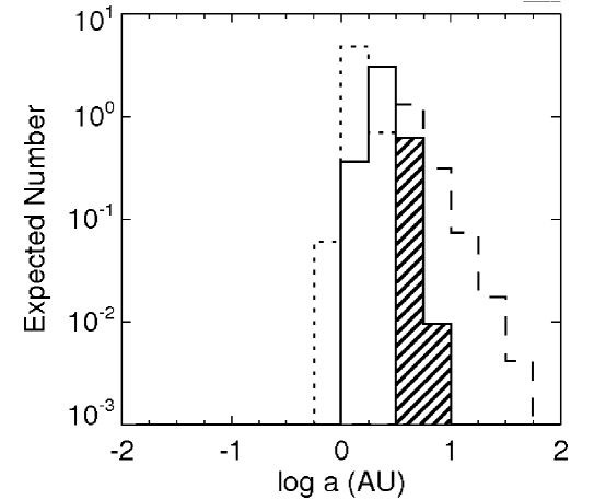
Figure 1: The expected number of one (solid line) and two (dotted line) transit events. The probability of observing exactly one or exactly two transits during the mission lifetime is convolved with the known distribution of semi-major axes. The shaded area indicates where this distribution is expected to be incomplete, and the dashed line shows our extrapolation to larger semi-major axes based on the flat distribution fit by Cumming et al. (2008).

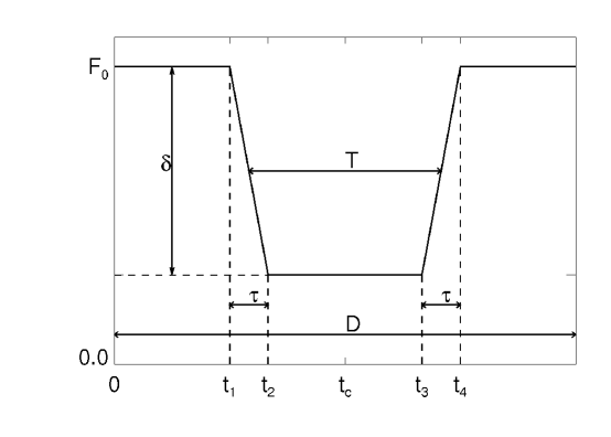
Figure 2: The model lightcurve. $t_{c}$ is the time of transit center, $T$ is the duration of the full-width half-maximum depth of the transit, $\tau$ is duration of ingress or egress, and $\delta$ is the fractional depth of the transit. $t_{1}$–$t_{4}$ are the points of contact. $F_{0}\equiv 1$ is the out-of-transit flux, and $D$ is the total duration of the observations.

2 Overview

We derive exact expressions for the uncertainties in $t_{c}$, $T$, $\tau$, and $\delta$, by applying the Fisher matrix formalism to the simple light curve model shown in Fig. 2 (Gould 2003). For the long-period transiting planets observed by Kepler, $\tau\ll T\ll D$ (the total duration of the observations), so the largest uncertainty is for $\tau$:

$$\frac{\sigma_{\tau}}{\tau}=Q^{-1}\sqrt{\frac{6T}{\tau}}.$$ (1)

Here $Q$ is approximately equal to the total signal-to-noise ratio of the transit,

$$Q\equiv(\Gamma_{\rm ph}T)^{1/2}\delta,$$ (2)

where $\Gamma_{\rm ph}$ is the photon collection rate. For a Jupiter-sized planet with period equal to the mission lifetime and transiting a $V=12$ solar-type star, $Q\simeq 1300$, whereas for a Neptune-sized planet, $Q\simeq 150$.

Assuming the planet is in a circular orbit, and the stellar density, $\rho_{\star}$, is known from spectroscopy, Seager & Mallén-Ornelas (2003) showed that the planet’s period, $P$, can be derived from a single observed transit,

$$P=\frac{2\pi a}{v_{\rm tr,p}}=\frac{G\pi^{2}}{3}\rho_{\star}\left(\frac{T\tau}{\sqrt{\delta}}\right)^{3/2}$$ (3)

where $v_{\rm tr,p}$ is the velocity of the planet at the time of transit.

Figure 3 shows contours of constant fractional uncertainty in the period as a function of $P$ and the planet radius, $r_{\rm p}$. The model assumes a solar-type star with $V=12.0$, an impact parameter b=0.2, and a 10% uncertainty in $\rho_{\star}$. The dashed line indicates how the fractional uncertainty in $P$ changes with $V$; it shows the 0.20 contour for $V=14.0$ and $b=0.2$. The diagonal dotted line shows the boundary below which the assumptions of the Fisher matrix break down (the ingress/egress time $\tau$ is roughly equal to the sampling rate of $1/dt=$ 1 observation/30 mins). The vertical dotted line shows the mission lifetime of Kepler ($L=$3.5 yrs). Solar system planets are indicated.

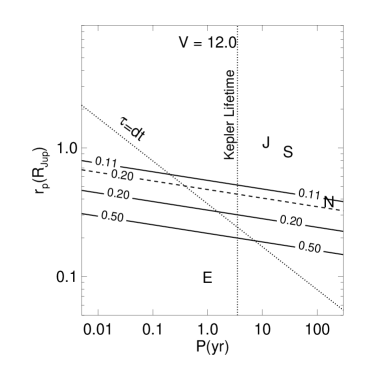
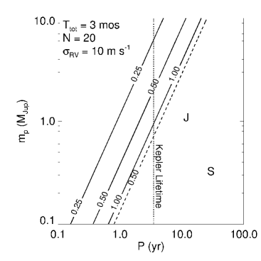
Figure 3: Left: Contours of constant fractional uncertainty in $P$: $\sigma_{P}/P$. Right: Contours of constant fractional uncertainty in $m_{\rm p}$: $\sigma_{m_{\rm p}}/m_{\rm p}$.

The mass of the planet can be estimated by sampling the stellar radial velocity (RV) curve soon after the transit is observed. Near the time of transit we can expand the stellar RV

$$v_{\star}\approx v_{0}-A_{\star}(t-t_{c}),$$ (4)

where $A_{\star}=2\pi K_{\star}/P$, and

$$K_{\star}=\left(\frac{2\pi G}{PM_{\star}^{2}}\right)^{1/3}m_{\rm p}\sin i$$ (5)

is the stellar radial velocity semi-amplitude and we assume $\sin i\approx 1$. The mass of the planet, $m_{\rm p}$, can be determined from the observables, $g_{\star}$, $A_{\star}$, $T$, $\tau$, and $\delta$:

$$m_{\rm p}=\frac{1}{16G}g_{\star}^{2}A_{\star}\left(\frac{T\tau}{\sqrt{\delta}}\right)^{2}.$$ (6)

Figure 3 shows contours of constant uncertainty in $m_{\rm p}$ as a function of $m_{\rm p}$ and $P$. The model assumes a 10% uncertainty in $g_{\star}$. The solid lines show the result for 20 radial velocity measurements with precision of 10 m s^-1 taken over a period of 3 months after the transit. The dashed line shows the 0.50 contour for 40 observations taken over 6 months. The dotted line indicates the mission lifetime of 3.5 years. The positions of Jupiter and Saturn are indicated.

If the eccentricity $e$ is non-zero, there is not a unique solution for $P$ and $m_{\rm p}$, however, we can still constrain them by adopting priors on $e$ and the argument of periastron $\omega_{\rm p}$. Using $e=0.3$ gives a range of inferred periods of 0.4–2.5 relative to the assumption of a circular orbit. The range of inferred masses is 0.5–1.7, which is smaller than the contribution from the uncertainty in $A_{\star}$.

In this paper, we demonstrated that it will be possible to detect and characterize long-period planets using observations of single transits by the Kepler satellite, combined with precise radial velocity measurements taken immediately after the transit. These results can also be generalized to any transiting planet survey, and it may be particularly interesting to apply them to the COnvection, ROtation & planetary Transits (CoRoT) mission (Baglin 2003). Additionally, estimates of the period of a transiting planet could allow the Kepler mission to make targeted increases in the sampling rate at the time of a second transit occurring during the mission.

References

- [Baglin(2003)] Baglin, A. 2003, Advances in Space Research, 31, 345
- [Basri et al. (2005)] Basri, G., Borucki, W. J., & Koch, D. 2005, New Astronomy Review, 49, 478
- [Borucki et al. (2004)] Borucki, W., Koch, D., Boss, A., Dunham, E., Dupree, A., Geary, J., Gilliland, R., Howell, S., Jenkins, J., Kondo, Y., Latham, D., Lissauer, J., & Reitsema, H. 2004, in ESA Special Publication, Vol. 538, Stellar Structure and Habitable Planet Finding, ed. F. Favata, S. Aigrain, & A. Wilson, 177–182
- [Cumming et al. (2008)] Cumming, A., Butler, R. P., Marcy, G. W., Vogt, S. S., Wright, J. T., & Fischer, D. A. 2008, arXiv:0803.3357, 803
- [Gould(2003)] Gould, A. 2003, arXiv:astro-ph/0310577
- [Seager & Mallén-Ornelas(2003)] Seager, S. & Mallén-Ornelas, G. 2003, ApJ, 585, 1038