New observables in the decay mode B¯dK¯+0subscript¯𝐵𝑑¯𝐾superscriptsuperscriptabsent0superscript\boldmath{\overline{\kern-2.40005ptB}_{d}\rightarrow\kern 1.99997pt\overline{\kern-1.99997ptK}{}^{*0}\ell^{+}\ell^{-}}

Ulrik Egede
Imperial College London, London SW7 2AZ, United Kingdom
E-mail
U.Egede@imperial.ac.uk
   Tobias Hurth
CERN, Dept. of Physics, Theory Division, CH-1211 Geneva 23, Switzerland
E-mail
Also SLAC, Stanford University, Stanford, CA 94309, USA. Tobias.Hurth@cern.ch
   Joaquim Matias
IFAE, Universitat Autònoma de Barcelona, 08193 Bellaterra, Barcelona, Spain
E-mail
matias@ifae.es
   Marc Ramon
IFAE, Universitat Autònoma de Barcelona, 08193 Bellaterra, Barcelona, Spain
E-mail
mramon@ifae.es
   Will Reece
Imperial College London, London SW7 2AZ, United Kingdom
E-mail
w.reece06@imperial.ac.uk
Abstract:

We discuss the large set of observables available from the angular distributions of the decay B¯dK¯+0subscript¯𝐵𝑑¯𝐾superscriptsuperscriptabsent0superscript\overline{\kern-2.40005ptB}_{d}\rightarrow\kern 1.99997pt\overline{\kern-1.99997ptK}{}^{*0}\ell^{+}\ell^{-}. We present a NLO analysis of all observables based on the QCD factorization approach in the low-dilepton mass region and an estimate of Λ/mbΛsubscript𝑚𝑏\mathchar 28931\relax/m_{b} corrections. Moreover, we discuss their sensitivity to new physics. We explore the experimental sensitivities at LHCb (10  fb1superscript fb1\mbox{\,fb}^{-1}) and SuperLHCb (100  fb1superscript fb1\mbox{\,fb}^{-1}) based on a full-angular fit method and explore the sensitivity to right handed currents. We also show that the previously discussed transversity amplitude AT(1)superscriptsubscript𝐴𝑇1A_{T}^{\left(1\right)} cannot be measured at the LHCb experiment or at future B𝐵B factory experiments as it requires a measurement of the spin of the final state particles.

B-Physics, Rare Decays
preprint: \arXivid0807.2589
UAB-FT-2008-652
CERN-TH/2008-155
SLAC-PUB-13307

1 Introduction

A major aim of particle physics in the LHC era is the discovery of new degrees of freedom at the TeVTeV\mathrm{\,Te\kern-1.00006ptV} energy scale which might contribute to our understanding of the origin of electroweak symmetry breaking. Rare B𝐵B and kaon decays (for reviews see [1, 2, 3]) representing loop-induced processes are highly sensitive probes for new degrees of freedom beyond the Standard Model (SM) and will be used when making indirect searches for these unknown effects. It is well-known that the indirect constraints on new physics (NP) from the present flavour data indicate a NP scale much higher than the electroweak scale when such new effects are naturally parameterised by higher-dimensional operators. Thus, if there is NP at the electroweak scale, then its flavour structure has to be highly non-trivial and the experimental measurement of flavour-violating couplings is mandatory. This ‘flavour problem’, namely why flavour-changing neutral currents are suppressed, has to be solved by any NP scenario at the electroweak scale.

In this article we discuss theoretical and experimental preparations for an indirect NP search using the rare decay B¯dK¯μ+0μsubscript¯𝐵𝑑¯𝐾superscriptsuperscript𝜇absent0superscript𝜇\kern 3.00003pt\overline{\kern-2.40005ptB}_{d}\rightarrow\kern 1.99997pt\overline{\kern-1.99997ptK}{}^{*0}\mu^{+}\mu^{-}. This exclusive decay was first observed at Belle [4]. It offers a rich phenomenology of various kinematical distributions beyond the measurement of the branching ratio. Some experimental analyses of those angular distributions are already presented by the B𝐵B factories [5, 6, 7, 8, 9] but only the large increase in statistics at LHCb [10, 11, 12] for B¯dK¯μ+0μsubscript¯𝐵𝑑¯𝐾superscriptsuperscript𝜇absent0superscript𝜇\kern 3.00003pt\overline{\kern-2.40005ptB}_{d}\rightarrow\kern 1.99997pt\overline{\kern-1.99997ptK}{}^{*0}\mu^{+}\mu^{-} will make much higher precision measurements possible. There are also great opportunities at the future (Super-)B𝐵B factories in this respect [13, 14, 15, 16]. A careful choice of observables needs to be made to take full advantage of this exclusive decay as only in certain ratios such as CP𝐶𝑃C\!P and forward-backward asymmetries, the hadronic uncertainties cancel out in specific observables making such ratios the only observables that are sensitive to NP. In this respect the by now standard theoretical tools like QCD factorization (QCDf) [17] and its quantum field theoretical formulation, soft-collinear effective theory (SCET), are crucial. They imply form factor relations which simplify the theoretical structure of various kinematical distributions such that at least at the leading order (LO) level any hadronic uncertainties cancel out. A well-known example of this is the zero-crossing of the forward-backward asymmetry.

We construct new observables of this kind in the B¯dK¯μ+0μsubscript¯𝐵𝑑¯𝐾superscriptsuperscript𝜇absent0superscript𝜇\kern 3.00003pt\overline{\kern-2.40005ptB}_{d}\rightarrow\kern 1.99997pt\overline{\kern-1.99997ptK}{}^{*0}\mu^{+}\mu^{-} decay which have very small theoretical uncertainties and good experimental resolution. Moreover, it is possible to design the new observables for a specific kind of NP operator within the model independent analysis using the effective field theory approach.

Previously proposed angular distributions and CP𝐶𝑃C\!P violating observables in B¯dK¯μ+0μsubscript¯𝐵𝑑¯𝐾superscriptsuperscript𝜇absent0superscript𝜇\kern 3.00003pt\overline{\kern-2.40005ptB}_{d}\rightarrow\kern 1.99997pt\overline{\kern-1.99997ptK}{}^{*0}\mu^{+}\mu^{-} are reviewed in Ref. [18, 15], and more recently QCDf analyses of such angular distributions [19, 20] and CP𝐶𝑃C\!P violating observables [21] were presented.

The paper is organised as follows: in Sec. 2 we recall the differential decay distribution in the B¯dK¯μ+0μsubscript¯𝐵𝑑¯𝐾superscriptsuperscript𝜇absent0superscript𝜇\kern 3.00003pt\overline{\kern-2.40005ptB}_{d}\rightarrow\kern 1.99997pt\overline{\kern-1.99997ptK}{}^{*0}\mu^{+}\mu^{-} decay; in Sec. 3 we recall the basic theoretical formulae which are crucial for our construction of new observables; in Sec. 4 we discuss the basic properties and symmetries of potential observables and propose a new set of observables which are sensitive to new right-handed currents and we also discuss the previously proposed quantity AT(1)superscriptsubscript𝐴𝑇1A_{T}^{(1)}; in Sec. 5 we explain our method to calculate the experimental sensitivity obtainable with the statistics of LHCb to new and old observables; and finally in Sec. 6 we present our phenomenological analysis, in particular we analyse the theoretical and experimental sensitivity to NP. We also comment very briefly on recent BABAR measurements of certain angular distributions. In appendices we make angular definitions explicit, provide the theoretical framework for the derivation of the spin amplitudes, and present the theoretical NLO expressions.

2 Differential decay distribution

The decay B¯dK¯+0subscript¯𝐵𝑑¯𝐾superscriptsuperscriptabsent0superscript\overline{\kern-2.40005ptB}_{d}\rightarrow\kern 1.99997pt\overline{\kern-1.99997ptK}{}^{*0}\ell^{+}\ell^{-} with K¯0Kπ+\kern 1.99997pt\overline{\kern-1.99997ptK}{}^{*0}\rightarrow K^{-}\pi^{+} on the mass shell, is completely described by four independent kinematic variables, the lepton-pair invariant mass squared, q2superscript𝑞2q^{2}, and the three angles θlsubscript𝜃𝑙\theta_{l}, θKsubscript𝜃𝐾\theta_{K}, ϕitalic-ϕ\phi. Summing over the spins of the final particles, the differential decay distribution of B¯dK¯+0subscript¯𝐵𝑑¯𝐾superscriptsuperscriptabsent0superscript\overline{\kern-2.40005ptB}_{d}\rightarrow\kern 1.99997pt\overline{\kern-1.99997ptK}{}^{*0}\ell^{+}\ell^{-} can be written as

d4ΓB¯ddq2dθldθKdϕ=932πI(q2,θl,θK,ϕ)sinθlsinθK,superscript𝑑4subscriptΓsubscript¯𝐵𝑑𝑑superscript𝑞2𝑑subscript𝜃𝑙𝑑subscript𝜃𝐾𝑑italic-ϕ932𝜋𝐼superscript𝑞2subscript𝜃𝑙subscript𝜃𝐾italic-ϕsubscript𝜃𝑙subscript𝜃𝐾\frac{d^{4}\Gamma_{\overline{\kern-1.68004ptB}_{d}}}{dq^{2}\,d\theta_{l}\,d\theta_{K}\,d\phi}=\frac{9}{32\pi}I(q^{2},\theta_{l},\theta_{K},\phi)\sin\theta_{l}\sin\theta_{K}\>, (1)

with the physical region of phase space 4ml2q2(mBmK)24superscriptsubscript𝑚𝑙2superscript𝑞2superscriptsubscript𝑚𝐵subscript𝑚superscript𝐾24m_{l}^{2}\leqslant q^{2}\leqslant(m_{B}-m_{K^{*}})^{2} and

I𝐼\displaystyle I =\displaystyle= I1+I2cos2θl+I3sin2θlcos2ϕ+I4sin2θlcosϕ+I5sinθlcosϕ+subscript𝐼1subscript𝐼22subscript𝜃𝑙subscript𝐼3superscript2subscript𝜃𝑙2italic-ϕsubscript𝐼42subscript𝜃𝑙italic-ϕlimit-fromsubscript𝐼5subscript𝜃𝑙italic-ϕ\displaystyle I_{1}+I_{2}\cos 2\theta_{l}+I_{3}\sin^{2}\theta_{l}\cos 2\phi+I_{4}\sin 2\theta_{l}\cos\phi+I_{5}\sin\theta_{l}\cos\phi+ (2)
+I6cosθl+I7sinθlsinϕ+I8sin2θlsinϕ+I9sin2θlsin2ϕ.subscript𝐼6subscript𝜃𝑙subscript𝐼7subscript𝜃𝑙italic-ϕsubscript𝐼82subscript𝜃𝑙italic-ϕsubscript𝐼9superscript2subscript𝜃𝑙2italic-ϕ\displaystyle+I_{6}\cos\theta_{l}+I_{7}\sin\theta_{l}\sin\phi+I_{8}\sin 2\theta_{l}\sin\phi+I_{9}\sin^{2}\theta_{l}\sin 2\phi.

The Iisubscript𝐼𝑖I_{i} depend on products of the seven complex Ksuperscript𝐾K^{*} spin amplitudes, AL/Rsubscript𝐴bottom𝐿𝑅A_{\bot L/R}, AL/RA_{\|L/R}, A0L/Rsubscript𝐴0𝐿𝑅A_{0L/R}, Atsubscript𝐴𝑡A_{t} (see next section) with each of these a function of q2superscript𝑞2q^{2}. Atsubscript𝐴𝑡A_{t} is related to the time-like component of the virtual Ksuperscript𝐾K^{*}, which does not contribute in the case of massless leptons and can be neglected if the lepton mass is small in comparison to the mass of the lepton pair. We will consider this case in our present analysis. For ml=0subscript𝑚𝑙0m_{l}=0, one finds [22, 23, 24, 25]:

I1subscript𝐼1\displaystyle I_{1} =\displaystyle= 34(|AL|2+|AL|2+(LR))sin2θK+(|A0L|2+|A0R|2)cos2θK\displaystyle\frac{3}{4}\left(|A_{\bot L}|^{2}+|A_{\|L}|^{2}+(L\rightarrow R)\right)\sin^{2}\theta_{K}+\left(|A_{0L}|^{2}+|A_{0R}|^{2}\right)\cos^{2}\theta_{K} (3a)
\displaystyle\equiv asin2θK+bcos2θK,𝑎superscript2subscript𝜃𝐾𝑏superscript2subscript𝜃𝐾\displaystyle a\sin^{2}\theta_{K}+b\cos^{2}\theta_{K},
I2subscript𝐼2\displaystyle I_{2} =\displaystyle= 14(|AL|2+|AL|2)sin2θK|A0L|2cos2θK+(LR)\displaystyle\frac{1}{4}(|A_{\bot L}|^{2}+|A_{\|L}|^{2})\sin^{2}\theta_{K}-|A_{0L}|^{2}\cos^{2}\theta_{K}+(L\rightarrow R) (3b)
\displaystyle\equiv csin2θK+dcos2θK,𝑐superscript2subscript𝜃𝐾𝑑superscript2subscript𝜃𝐾\displaystyle c\sin^{2}\theta_{K}+d\cos^{2}\theta_{K},
I3subscript𝐼3\displaystyle I_{3} =\displaystyle= 12[(|AL|2|AL|2)sin2θK+(LR)]esin2θK,\displaystyle\frac{1}{2}\bigg{[}(|A_{\bot L}|^{2}-|A_{\|L}|^{2})\sin^{2}\theta_{K}+(L\rightarrow R)\bigg{]}\equiv e\sin^{2}\theta_{K}, (3c)
I4subscript𝐼4\displaystyle I_{4} =\displaystyle= 12[Re(A0LAL)sin2θK+(LR)]fsin2θK,\displaystyle\frac{1}{\sqrt{2}}\bigg{[}{\text{Re}}(A_{0L}A_{\|L}^{*})\sin 2\theta_{K}+(L\rightarrow R)\bigg{]}\equiv f\sin 2\theta_{K}, (3d)
I5subscript𝐼5\displaystyle I_{5} =\displaystyle= 2[Re(A0LAL)sin2θK(LR)]gsin2θK,2delimited-[]Resubscript𝐴0𝐿superscriptsubscript𝐴bottom𝐿2subscript𝜃𝐾𝐿𝑅𝑔2subscript𝜃𝐾\displaystyle\sqrt{2}\bigg{[}{\text{Re}}(A_{0L}A_{\bot L}^{*})\sin 2\theta_{K}-(L\rightarrow R)\bigg{]}\equiv g\sin 2\theta_{K}, (3e)
I6subscript𝐼6\displaystyle I_{6} =\displaystyle= 2[Re(ALAL)sin2θK(LR)]hsin2θK,\displaystyle 2\bigg{[}{\text{Re}}(A_{\|L}A_{\bot L}^{*})\sin^{2}\theta_{K}-(L\rightarrow R)\bigg{]}\equiv h\sin^{2}\theta_{K}, (3f)
I7subscript𝐼7\displaystyle I_{7} =\displaystyle= 2[Im(A0LAL)sin2θK(LR)]jsin2θK,\displaystyle\sqrt{2}\bigg{[}{\text{Im}}(A_{0L}A_{\|L}^{*})\sin 2\theta_{K}-(L\rightarrow R)\bigg{]}\equiv j\sin 2\theta_{K}, (3g)
I8subscript𝐼8\displaystyle I_{8} =\displaystyle= 12[Im(A0LAL)sin2θK+(LR)]ksin2θK,12delimited-[]Imsubscript𝐴0𝐿superscriptsubscript𝐴bottom𝐿2subscript𝜃𝐾𝐿𝑅𝑘2subscript𝜃𝐾\displaystyle\frac{1}{\sqrt{2}}\bigg{[}{\text{Im}}(A_{0L}A_{\bot L}^{*})\sin 2\theta_{K}+(L\rightarrow R)\bigg{]}\equiv k\sin 2\theta_{K}, (3h)
I9subscript𝐼9\displaystyle I_{9} =\displaystyle= [Im(ALAL)sin2θK+(LR)]msin2θK.\displaystyle\bigg{[}{\text{Im}}(A_{\|L}^{*}A_{\bot L})\sin^{2}\theta_{K}+(L\rightarrow R)\bigg{]}\equiv m\sin^{2}\theta_{K}. (3i)

The exact equations presented here depend on the definition of the angles which we for this reason have made explicit in Appendix A.

From comparing the amplitude terms in Eq. (3), we see that a=3c𝑎3𝑐a=3c and b=d𝑏𝑑b=-d thus leaving nine independent parameters which can be fixed experimentally in a full angular fit. Assuming massless leptons in the theory we have on the other hand 12 parameters from the six complex K¯0\kern 1.99997pt\overline{\kern-1.99997ptK}{}^{*0} spin amplitudes, AL/Rsubscript𝐴bottom𝐿𝑅A_{\bot L/R}, AL/RA_{\|L/R}, A0L/Rsubscript𝐴0𝐿𝑅A_{0L/R}. See Sec. 4 for an analysis of the apparent mismatch between the 9 and 12 parameters.

3 Ksuperscript𝐾K^{*} spin amplitudes

The six complex Ksuperscript𝐾K^{*} spin amplitudes under the assumption of massless leptons are related to the well-known helicity amplitudes (used for example in [23, 24, 26]) through

A,=(H+1H1)/2,A0=H0.A_{\bot,\|}=(H_{+1}\mp H_{-1})/\sqrt{2}\,,\qquad A_{0}=H_{0}. (4)

The amplitudes describe the BKπ𝐵𝐾𝜋B\rightarrow K\pi transition and can be parameterised in terms of the seven BK𝐵superscript𝐾B\rightarrow K^{*} form factors by means of a narrow-width approximation. They also depend on the short-distance Wilson coefficients Cisubscript𝐶𝑖C_{i} corresponding to the various operators of the effective electroweak Hamiltonian. The precise definitions of the form factors and of the effective operators are given in Appendix B. One obtains [19]

AL,R=N2λ1/2[(𝒞9(eff)𝒞10)V(q2)mB+mK+2mbq2(𝒞7(eff)+𝒞7(eff))T1(q2)],A_{\bot L,R}=N\sqrt{2}\lambda^{1/2}\bigg{[}(\mathcal{C}_{9}^{\mathrm{(eff)}}\mp\mathcal{C}_{10})\frac{V(q^{2})}{m_{B}+m_{K^{*}}}+\frac{2m_{b}}{q^{2}}(\mathcal{C}_{7}^{\mathrm{(eff)}}+\mathcal{C}_{7}^{{}^{\prime}\mathrm{(eff)}})T_{1}(q^{2})\bigg{]}, (5)
AL,R=N2(mB2mK2)[(𝒞9(eff)𝒞10)A1(q2)mBmK+2mbq2(𝒞7(eff)𝒞7(eff))T2(q2)],A_{\|L,R}=-N\sqrt{2}(m_{B}^{2}-m_{K^{*}}^{2})\bigg{[}(\mathcal{C}_{9}^{\mathrm{(eff)}}\mp\mathcal{C}_{10})\frac{A_{1}(q^{2})}{m_{B}-m_{K^{*}}}+\frac{2m_{b}}{q^{2}}(\mathcal{C}_{7}^{\mathrm{(eff)}}-\mathcal{C}_{7}^{{}^{\prime}\mathrm{(eff)}})T_{2}(q^{2})\bigg{]}, (6)
A0L,Rsubscript𝐴0𝐿𝑅\displaystyle A_{0L,R} =\displaystyle= N2mKq2×\displaystyle-\frac{N}{2m_{K^{*}}\sqrt{q^{2}}}\times (7)
×[(𝒞9(eff)𝒞10){(mB2mK2q2)(mB+mK)A1(q2)\displaystyle\times\bigg{[}(\mathcal{C}_{9}^{\mathrm{(eff)}}\mp\mathcal{C}_{10})\bigg{\{}(m_{B}^{2}-m_{K^{*}}^{2}-q^{2})(m_{B}+m_{K^{*}})A_{1}(q^{2})-
λA2(q2)mB+mK}+\displaystyle\qquad\qquad\qquad\qquad-\lambda\frac{A_{2}(q^{2})}{m_{B}+m_{K^{*}}}\bigg{\}}+
+2mb(𝒞7(eff)𝒞7(eff)){(mB2+3mK2q2)T2(q2)\displaystyle\quad\ +{2m_{b}}(\mathcal{C}_{7}^{\mathrm{(eff)}}-\mathcal{C}_{7}^{{}^{\prime}\mathrm{(eff)}})\bigg{\{}(m_{B}^{2}+3m_{K^{*}}^{2}-q^{2})T_{2}(q^{2})-
λmB2mK2T3(q2)}],\displaystyle\qquad\qquad\qquad\qquad\qquad\quad-\frac{\lambda}{m_{B}^{2}-m_{K^{*}}^{2}}T_{3}(q^{2})\bigg{\}}\bigg{]},

where

λ=mB4+mK4+q42(mB2mK2+mK2q2+mB2q2)𝜆superscriptsubscript𝑚𝐵4superscriptsubscript𝑚superscript𝐾4superscript𝑞42superscriptsubscript𝑚𝐵2superscriptsubscript𝑚superscript𝐾2superscriptsubscript𝑚superscript𝐾2superscript𝑞2superscriptsubscript𝑚𝐵2superscript𝑞2\lambda=m_{B}^{4}+m_{K^{*}}^{4}+q^{4}-2(m_{B}^{2}m_{K^{*}}^{2}+m_{K^{*}}^{2}q^{2}+m_{B}^{2}q^{2}) (8)

and

N=GF2α23210π5mB3|VtbVts|2q2λ1/214ml2q2.𝑁superscriptsubscript𝐺𝐹2superscript𝛼23superscript210superscript𝜋5superscriptsubscript𝑚𝐵3superscriptsubscript𝑉𝑡𝑏superscriptsubscript𝑉𝑡𝑠2superscript𝑞2superscript𝜆1214superscriptsubscript𝑚𝑙2superscript𝑞2N=\sqrt{\frac{G_{F}^{2}\alpha^{2}}{3\cdot 2^{10}\pi^{5}m_{B}^{3}}|V_{tb}V_{ts}^{\ast}|^{2}q^{2}\lambda^{1/2}\sqrt{1-\frac{4m_{l}^{2}}{q^{2}}}}. (9)

The crucial theoretical input we use in our analysis is the observation that in the limit where the initial hadron is heavy and the final meson has a large energy [27] the hadronic form factors can be expanded in the small ratios ΛQCD/mbsubscriptΛQCDsubscript𝑚𝑏\mathchar 28931\relax_{\mathrm{QCD}}/m_{b} and ΛQCD/EsubscriptΛQCD𝐸\mathchar 28931\relax_{\mathrm{QCD}}/E, where E𝐸E is the energy of the light meson. Neglecting corrections of order 1/mb1subscript𝑚𝑏1/m_{b} and αssubscript𝛼𝑠\alpha_{s}, the seven a priori independent BK𝐵superscript𝐾B\rightarrow K^{*} form factors reduce to two universal form factors ξsubscript𝜉bottom\xi_{\bot} and ξsubscript𝜉\xi_{\|} [27, 28]. These relations can be strictly derived within the QCDf and SCET approach and are given in the appendix. Using those simplifications the spin amplitudes at leading order in 1/mb1subscript𝑚𝑏1/m_{b} and αssubscript𝛼𝑠\alpha_{s} have a very simple form:

AL,R=2NmB(1s^)[(𝒞9(eff)𝒞10)+2m^bs^(𝒞7(eff)+𝒞7(eff))]ξ(EK),A_{\bot L,R}=\sqrt{2}Nm_{B}(1-\hat{s})\bigg{[}(\mathcal{C}_{9}^{\mathrm{(eff)}}\mp\mathcal{C}_{10})+\frac{2\hat{m}_{b}}{\hat{s}}(\mathcal{C}_{7}^{\mathrm{(eff)}}+\mathcal{C}_{7}^{{}^{\prime}\mathrm{(eff)}})\bigg{]}\xi_{\bot}(E_{K^{*}}), (10)
AL,R=2NmB(1s^)[(𝒞9(eff)𝒞10)+2m^bs^(𝒞7(eff)𝒞7(eff))]ξ(EK),A_{\|L,R}=-\sqrt{2}Nm_{B}(1-\hat{s})\bigg{[}(\mathcal{C}_{9}^{\mathrm{(eff)}}\mp\mathcal{C}_{10})+\frac{2\hat{m}_{b}}{\hat{s}}(\mathcal{C}_{7}^{\mathrm{(eff)}}-\mathcal{C}_{7}^{{}^{\prime}\mathrm{(eff)}})\bigg{]}\xi_{\bot}(E_{K^{*}})\,, (11)
A0L,R=NmB2m^Ks^(1s^)2[(𝒞9(eff)𝒞10)+2m^b(𝒞7(eff)𝒞7(eff))]ξ(EK),A_{0L,R}=-\frac{Nm_{B}}{2\hat{m}_{K^{*}}\sqrt{\hat{s}}}(1-\hat{s})^{2}\bigg{[}(\mathcal{C}_{9}^{\mathrm{(eff)}}\mp\mathcal{C}_{10})+2\hat{m}_{b}(\mathcal{C}_{7}^{\mathrm{(eff)}}-\mathcal{C}_{7}^{{}^{\prime}\mathrm{(eff)}})\bigg{]}\xi_{\|}(E_{K^{*}})\,, (12)

with s^=q2/mB2^𝑠superscript𝑞2superscriptsubscript𝑚𝐵2\hat{s}=q^{2}/m_{B}^{2}, m^i=mi/mBsubscript^𝑚𝑖subscript𝑚𝑖subscript𝑚𝐵\hat{m}_{i}=m_{i}/m_{B}. Here we neglected terms of O(m^K2)𝑂superscriptsubscript^𝑚superscript𝐾2O(\hat{m}_{K^{*}}^{2}).

Some remarks are in order:

  • The theoretical simplifications are restricted to the kinematic region in which the energy of the Ksuperscript𝐾K^{*} is of the order of the heavy quark mass, i.e. q2mB2much-less-thansuperscript𝑞2superscriptsubscript𝑚𝐵2q^{2}\ll m_{B}^{2}. Moreover, the influences of very light resonances below 1GeV2superscriptGeV2{\mathrm{\,Ge\kern-1.00006ptV^{2}}} question the QCD factorization results in that region. Thus, we will confine our analysis of all observables to the dilepton mass in the range, 1GeV2q26GeV21superscriptGeV2superscript𝑞26superscriptGeV21{\mathrm{\,Ge\kern-1.00006ptV^{2}}}\leqslant q^{2}\leqslant 6{\mathrm{\,Ge\kern-1.00006ptV^{2}}}.

  • Within the SM, we recover the naive quark-model prediction of A=Asubscript𝐴bottomsubscript𝐴A_{\bot}=-A_{\|} [29, 30] in the mBsubscript𝑚𝐵m_{B}\rightarrow\infty and EKsubscript𝐸superscript𝐾E_{K^{*}}\rightarrow\infty limit (equivalently m^K20superscriptsubscript^𝑚superscript𝐾20\hat{m}_{K^{*}}^{2}\rightarrow 0). In this case, the s𝑠s quark is produced in helicity 1/212-{1}/{2} by weak interactions in the limit ms0subscript𝑚𝑠0m_{s}\rightarrow 0, which is not affected by strong interactions in the massless case [31]. Thus, the strange quark combines with a light quark to form a Ksuperscript𝐾K^{*} with helicity either 11-1 or 00 but not +11+1. Consequently, the SM predicts at quark level H+1=0subscript𝐻10H_{+1}=0, and hence A=Asubscript𝐴bottomsubscript𝐴A_{\bot}=-A_{\|} [cf. Eq. (4)], which is revealed as |H1||H+1|much-greater-thansubscript𝐻1subscript𝐻1|H_{-1}|\gg|H_{+1}| (or AAsubscript𝐴bottomsubscript𝐴A_{\bot}\approx-A_{\|}) at the hadron level.

  • As noted in Ref. [19], the contributions of the chirality-flipped operators 𝒪9,10=𝒪9,10(PLPR)superscriptsubscript𝒪910subscript𝒪910subscript𝑃𝐿subscript𝑃𝑅{\mathcal{O}}_{9,10}^{\prime}={\mathcal{O}}_{9,10}(P_{L}\rightarrow P_{R}) can be included in the above amplitudes by the replacements 𝒞9,10(eff)𝒞9,10(eff)+𝒞9,10(eff)\mathcal{C}_{9,10}^{\mathrm{(eff)}}\rightarrow\mathcal{C}_{9,10}^{\mathrm{(eff)}}+\mathcal{C}_{9,10}^{{}^{\prime}\mathrm{(eff)}} in Eq. (10), 𝒞9,10(eff)𝒞9,10(eff)𝒞9,10(eff)\mathcal{C}_{9,10}^{\mathrm{(eff)}}\rightarrow\mathcal{C}_{9,10}^{\mathrm{(eff)}}-\mathcal{C}_{9,10}^{{}^{\prime}\mathrm{(eff)}} in Eqs. (11) and (12). However, they play a sub-dominant role in our NP analysis presented here.

  • The symmetry breaking corrections of order αssubscript𝛼𝑠\alpha_{s} can be calculated in the QCDf/SCET approach. Those NLO corrections are included in our numerical analysis following Ref. [17]. The corresponding formulae for the case 𝒞7(eff)0\mathcal{C}_{7}^{{}^{\prime}\mathrm{(eff)}}\neq 0 are given in Appendix C.

  • In general we have no means to calculate Λ/mbΛsubscript𝑚𝑏\mathchar 28931\relax/m_{b} corrections to the QCDf amplitudes so they are treated as unknown corrections. This leads to a large uncertainty of theoretical predictions based on the QCDf/SCET approach. However, in specific examples one can combine QCDf/SCET results with calculations based on the QCD sum rule approach in order to estimate the leading power corrections.

    To take into account the present situation, we introduce a set of extra parameters, one for each spin amplitude, to explore what the effect of a possible Λ/mbΛsubscript𝑚𝑏\mathchar 28931\relax/m_{b} correction could be:

    A,,0=A,,00(1+c,,0)A_{\bot,\|,0}=A_{\bot,\|,0}^{0}\left(1+c_{\bot,\|,0}\right) (13)

    where the ‘0’ superscript stands for the QCD NLO Factorization amplitude and c,,0c_{\bot,\|,0} are taken to vary in a range ±10%plus-or-minuspercent10\pm 10\% which corresponds to a naive dimensional estimate. For each observable we look at, each of the amplitudes were varied in turn leaving the others at their central value. All the variations were then added in quadrature. Furthermore, we also give our final predictions taking into account further improvements on the power corrections and varying the independent parameters in a less conservative range of ±5%plus-or-minuspercent5\pm 5\%.

4 Theoretically clean observables

4.1 General criteria

We recall again that 2 of the 11 measurable distribution functions a,b,,m𝑎𝑏𝑚a,b,\dots,m of the differential decay distribution in the limit m2q2much-less-thansuperscriptsubscript𝑚2superscript𝑞2m_{\ell}^{2}\ll q^{2}, defined in Eq. 3, include redundant information due to the relations a=3c𝑎3𝑐a=3c and b=d𝑏𝑑b=-d. So in principle there are 9 independent observables. However, the dependence of those functions on the six complex theoretical spin amplitudes, AL/Rsubscript𝐴bottom𝐿𝑅A_{\bot L/R}, AL/RA_{\|L/R} and A0L/Rsubscript𝐴0𝐿𝑅A_{0L/R}, is special. By inspection one finds that the distribution functions are invariant under the following three independent symmetry transformations of the spin amplitudes: global phase transformation of the L𝐿L-amplitudes

AL=eiϕLAL,AL=eiϕLAL,A0L=eiϕLA0L,A^{{}^{\prime}}_{\bot L}=e^{i\phi_{L}}A_{\bot L},\qquad A^{{}^{\prime}}_{\|L}=e^{i\phi_{L}}A_{\|L},\qquad A^{{}^{\prime}}_{0L}=e^{i\phi_{L}}A_{0L}, (14)

global phase transformation of the R𝑅R-amplitudes

AR=eiϕRAR,AR=eiϕRAR,A0R=eiϕRA0R,A^{{}^{\prime}}_{\bot R}=e^{i\phi_{R}}A_{\bot R},\qquad A^{{}^{\prime}}_{\|R}=e^{i\phi_{R}}A_{\|R},\qquad A^{{}^{\prime}}_{0R}=e^{i\phi_{R}}A_{0R}, (15)

and a continuous LR𝐿𝑅L\leftrightarrow R rotation

ALsubscriptsuperscript𝐴bottom𝐿\displaystyle A^{{}^{\prime}}_{\bot L} =\displaystyle= +cosθAL+sinθAR𝜃subscript𝐴bottom𝐿𝜃subscriptsuperscript𝐴bottom𝑅\displaystyle+\cos\theta A_{\bot L}+\sin\theta A^{*}_{\bot R} (16a)
ARsubscriptsuperscript𝐴bottom𝑅\displaystyle A^{{}^{\prime}}_{\bot R} =\displaystyle= sinθAL+cosθAR𝜃subscriptsuperscript𝐴bottom𝐿𝜃subscript𝐴bottom𝑅\displaystyle-\sin\theta A^{*}_{\bot L}+\cos\theta A_{\bot R} (16b)
A0Lsubscriptsuperscript𝐴0𝐿\displaystyle A^{{}^{\prime}}_{0L} =\displaystyle= +cosθA0LsinθA0R𝜃subscript𝐴0𝐿𝜃subscriptsuperscript𝐴0𝑅\displaystyle+\cos\theta A_{0L}-\sin\theta A^{*}_{0R} (16c)
A0Rsubscriptsuperscript𝐴0𝑅\displaystyle A^{{}^{\prime}}_{0R} =\displaystyle= +sinθA0L+cosθA0R𝜃subscriptsuperscript𝐴0𝐿𝜃subscript𝐴0𝑅\displaystyle+\sin\theta A^{*}_{0L}+\cos\theta A_{0R} (16d)
AL\displaystyle A^{{}^{\prime}}_{\|L} =\displaystyle= +cosθALsinθAR\displaystyle+\cos\theta A_{\|L}-\sin\theta A^{*}_{\|R} (16e)
AR\displaystyle A^{{}^{\prime}}_{\|R} =\displaystyle= +sinθAL+cosθAR.\displaystyle+\sin\theta A^{*}_{\|L}+\cos\theta A_{\|R}\,. (16f)

Normally, there is the freedom to pick a single global phase, but as L𝐿L and R𝑅R amplitudes do not interfere here, two phases can be chosen arbitrarily as reflected in the first two transformations. The third symmetry reflects that an average is made over the spin amplitudes to obtain the angular distribution. So it is clear that only 999 out of the 121212 parameters arising from the 6 complex amplitudes are independent which fits exactly with the 999 independent measurable distribution functions.

A consequence of the three symmetries is that any observable based on the differential decay distribution has also to be invariant under the same symmetry transformations.

Besides the mandatory criterion above there are further criteria required for an interesting observable:

Simplicity:

A simple functional dependence on the 9 independent measurable distribution functions; at best it should depend only from one or two in the numerator and denominator of an asymmetry.

Cleanliness:

At leading order in Λ/mbΛsubscript𝑚𝑏\mathchar 28931\relax/m_{b} and in αssubscript𝛼𝑠\alpha_{s} the observable should be independent of any form factor, at best for all q2superscript𝑞2q^{2}. Also the influence of symmetry-breaking corrections at order αssubscript𝛼𝑠\alpha_{s} and at order Λ/mbΛsubscript𝑚𝑏\mathchar 28931\relax/m_{b} should be minimal.

Sensitivity:

The sensitivity to the 𝒞7(eff)\mathcal{C}_{7}^{{}^{\prime}\mathrm{(eff)}} Wilson coefficient representing NP with another chirality than in the SM should be maximal.

Precision:

The experimental precision obtainable should be good enough to distinguish different NP models.

In the limit where the K¯0\kern 1.99997pt\overline{\kern-1.99997ptK}{}^{*0} meson has a large energy, only two independent form factors occur in A0L/Rsubscript𝐴0𝐿𝑅A_{0L/R} and in AL/Rsubscript𝐴bottom𝐿𝑅A_{\bot L/R} and AL/RA_{\|L/R}. Clearly, any ratio of two of the nine measurable distribution functions proportional to the same form factor fulfil the criterion of symmetry, simplicity, and theoretical cleanliness up to Λ/mbΛsubscript𝑚𝑏\mathchar 28931\relax/m_{b} and αssubscript𝛼𝑠\alpha_{s} corrections. However, the third criterion, a sensitivity to a special kind of NP and the subsequent requirement of experimental precision, singles out particular combinations. In this paper we focus on new right-handed currents. Other NP sensitivities may single out other observables as will be analysed in a forthcoming paper [32].

4.2 Observables

There are some proposals for theoretical clean observables already in the literature which we should briefly discuss in view of the above criteria:

  • The forward backward asymmetry is the most popular quantity in the B¯dK¯μ+0μsubscript¯𝐵𝑑¯𝐾superscriptsuperscript𝜇absent0superscript𝜇\kern 3.00003pt\overline{\kern-2.40005ptB}_{d}\rightarrow\kern 1.99997pt\overline{\kern-1.99997ptK}{}^{*0}\mu^{+}\mu^{-} decay [33]. In terms of the K¯0\kern 1.99997pt\overline{\kern-1.99997ptK}{}^{*0} spin amplitudes it can be written as [17, 34]

    AFB=32Re(ALAL)Re(ARAR)|A0|2+|A|2+|A|2A_{\mathrm{FB}}=\frac{3}{2}\frac{{\text{Re}}(A_{\|L}A_{\bot L}^{*})-{\text{Re}}(A_{\|R}A_{\bot R}^{*})}{|A_{0}|^{2}+|A_{\|}|^{2}+|{A}_{\bot}|^{2}} (17)

    where

    AiAjAiL(q2)AjL(q2)+AiR(q2)AjR(q2)(i,j=0,,).A_{i}A^{*}_{j}\equiv A_{iL}(q^{2})A^{*}_{jL}(q^{2})+A_{iR}(q^{2})A^{*}_{jR}(q^{2})\quad(i,j=0,\|,\perp)\,. (18)

    While the criteria of symmetry and simplicity are fulfilled, the form factors cancel out only at the specific value of q2superscript𝑞2q^{2} where AFB=0subscript𝐴FB0A_{\mathrm{FB}}=0. Thus the measurement provide only a single clean number, the zero crossing point, rather than a theoretically clean distribution.

  • The fractions of the K¯0\kern 1.99997pt\overline{\kern-1.99997ptK}{}^{*0} polarisation

    FL(q2)subscript𝐹𝐿superscript𝑞2\displaystyle F_{L}(q^{2}) =\displaystyle= |A0|2|A0|2+|A|2+|A|2,superscriptsubscript𝐴02superscriptsubscript𝐴02superscriptsubscript𝐴2superscriptsubscript𝐴perpendicular-to2\displaystyle\frac{|{A}_{0}|^{2}}{|{A}_{0}|^{2}+|{A}_{\|}|^{2}+|A_{\perp}|^{2}}, (19)
    FT(q2)subscript𝐹𝑇superscript𝑞2\displaystyle F_{T}(q^{2}) =\displaystyle= 1FL(q2)=|A|2+|A|2|A0|2+|A|2+|A|2,1subscript𝐹𝐿superscript𝑞2superscriptsubscript𝐴bottom2superscriptsubscript𝐴2superscriptsubscript𝐴02superscriptsubscript𝐴2superscriptsubscript𝐴perpendicular-to2\displaystyle 1-F_{L}(q^{2})=\frac{|{A}_{\bot}|^{2}+|{A}_{\|}|^{2}}{|{A}_{0}|^{2}+|{A}_{\|}|^{2}+|A_{\perp}|^{2}}\,, (20)

    and the Ksuperscript𝐾K^{*} polarisation parameter

    αK(q2)=2FLFT1=2|A0|2|A|2+|A|21.subscript𝛼superscript𝐾superscript𝑞22subscript𝐹𝐿subscript𝐹𝑇12superscriptsubscript𝐴02superscriptsubscript𝐴2superscriptsubscript𝐴perpendicular-to21\alpha_{K^{*}}(q^{2})=\frac{2F_{L}}{F_{T}}-1=\frac{2|{A}_{0}|^{2}}{|{A}_{\|}|^{2}+|{A}_{\perp}|^{2}}-1\,. (21)

    All fulfil the criteria of symmetry and simplicity, but the form factors do not cancel in the LO approximation; thus, suffering from larger hadronic uncertainties. The fraction of the K¯\kern 1.99997pt\overline{\kern-1.99997ptK}{}^{*} polarisation can be measured from the angular projections alone and the first experimental measurements of FLsubscript𝐹𝐿F_{L} with limited accuracy are available [8, 9].

  • Defining the helicity distributions Γ±=|H±1L|2+|H±1R|2subscriptΓplus-or-minussuperscriptsubscriptsuperscript𝐻𝐿plus-or-minus12superscriptsubscriptsuperscript𝐻𝑅plus-or-minus12\Gamma_{\pm}=|H^{L}_{\pm 1}|^{2}+|H^{R}_{\pm 1}|^{2} one can construct [23]

    AT(1)=ΓΓ+Γ+Γ+=2Re(AA)|A|2+|A|2.superscriptsubscript𝐴𝑇1subscriptΓsubscriptΓsubscriptΓsubscriptΓ2Resubscript𝐴superscriptsubscript𝐴bottomsuperscriptsubscript𝐴bottom2superscriptsubscript𝐴2A_{T}^{\left(1\right)}=\frac{\Gamma_{-}-\Gamma_{+}}{\Gamma_{-}+\Gamma_{+}}=\frac{-2{\text{Re}}(A_{\|}{A}_{\bot}^{*})}{|{A}_{\bot}|^{2}+|A_{\|}|^{2}}\,. (22)

    It has been shown[19, 20] that this quantity has adequate cleanliness and is is very sensitive to right-handed currents, making an ideal observable if just these two criteria were sufficient. However, the quantity AT(1)superscriptsubscript𝐴𝑇1A_{T}^{\left(1\right)} does not fulfil the most important criterion of symmetry. The important consequences out of this observation are briefly discussed in the next subsection.

  • The other transversity amplitude, first proposed in [19], is defined as

    AT(2)=|A|2|A|2|A|2+|A|2.superscriptsubscript𝐴𝑇2superscriptsubscript𝐴bottom2superscriptsubscript𝐴2superscriptsubscript𝐴bottom2superscriptsubscript𝐴2A_{T}^{\left(2\right)}=\frac{|{A}_{\bot}|^{2}-|A_{\|}|^{2}}{|{A}_{\bot}|^{2}+|A_{\|}|^{2}}\,. (23)

    It obviously fulfils all three criteria of symmetry, simplicity and theoretical cleanliness. It is also rather sensitivity to 𝒞7(eff)\mathcal{C}_{7}^{{}^{\prime}\mathrm{(eff)}} as one can see by inspection of the LO formulae of the K¯0\kern 1.99997pt\overline{\kern-1.99997ptK}{}^{*0} amplitudes in Eqs. (10-12); in this approximation it is directly proportional to 𝒞7(eff)\mathcal{C}_{7}^{{}^{\prime}\mathrm{(eff)}}, thus vanishes in the SM.

By inspection of the formulae of the Ksuperscript𝐾K^{*} spin amplitudes in terms of the Wilson coefficients and the SCET form factors at the LO approximation, Eqs. (10-12), one is led to some new observables which fulfil the first three criteria and have an enhanced sensitivity to 𝒞7(eff)\mathcal{C}_{7}^{{}^{\prime}\mathrm{(eff)}}. They are defined as

AT(3)=|A0LAL+A0RAR||A0|2|A|2,A_{T}^{\left(3\right)}=\frac{|A_{0L}A_{\|L}^{*}+A_{0R}^{*}A_{\|R}|}{\sqrt{|A_{0}|^{2}|{A}_{\bot}|^{2}}}\,, (24)

and

AT(4)=|A0LALA0RAR||A0LAL+A0RAR|,A_{T}^{\left(4\right)}=\frac{|A_{0L}A_{\perp L}^{*}-A_{0R}^{*}A_{\perp R}|}{|A_{0L}^{*}A_{\|L}+A_{0R}A_{\|R}^{*}|}\,, (25)

One could also consider the real and imaginary parts of AT(3)superscriptsubscript𝐴𝑇3A_{T}^{\left(3\right)}.

There are no further independent quantities which fulfil the criteria we have set out. However, when we will consider NP sensitivities beyond 𝒞7(eff)\mathcal{C}_{7}^{{}^{\prime}\mathrm{(eff)}} further observables may be singled out [32].

4.3 The problem with 𝑨𝑻(𝟏)superscriptsubscript𝑨𝑻1A_{T}^{\left(1\right)}

Contrary to the case of AT(i)superscriptsubscript𝐴𝑇𝑖A_{T}^{\left(i\right)} with i=2,3,4𝑖234i=2,3,4, it is not possible to extract AT(1)superscriptsubscript𝐴𝑇1A_{T}^{\left(1\right)} from the full angular distribution. This is a direct consequence of the fact that the quantity AT(1)superscriptsubscript𝐴𝑇1A_{T}^{\left(1\right)} is not invariant under the symmetry (16) of the distribution function (1) which represent the complete set of observables in the case spins of the final states are summed up. Let us elaborate further on this surprising observation; it seems practically not possible to measure the helicity of the final states on a event-by-event basis. At the forthcoming LHCb experiment for example one only measures the charge, the three-momentum of the final state particles and its nature through different types of particle identification. So one has the four-momentum for each particle and its charge. The situation does not look different for the present B𝐵B factories and their future upgrades. While the e+esuperscript𝑒superscript𝑒e^{+}e^{-} environment is much simpler there is still no practical way to measure the spin of the muons on an event-by-event basis. We should emphasise that this is a practical and not a conceptual problem; in a gedanken experiment where the helicity of the individual final state leptons are measured, it would indeed be possible to measure AT(1)superscriptsubscript𝐴𝑇1A_{T}^{\left(1\right)}. So while AT(1)superscriptsubscript𝐴𝑇1A_{T}^{\left(1\right)} is in principle a good observable, we cannot see any way it can be measured at either LHCb or at a Super-B𝐵B factory with electrons or muons in the final state.

5 Method to calculate experimental sensitivity

In this section we explain how to investigate the sensitivity to the angular observables presented in Sec. 4 using a toy Monte Carlo model. We estimate the statistical uncertainty on all observables with statistics corresponding to 5 years of nominal running at LHCb (10 fb1superscript fb1\mbox{\,fb}^{-1}) and comment on the experimental prospects for a measurement at the end of an upgrade to LHCb (100 fb1superscript fb1\mbox{\,fb}^{-1}). For the estimates here we are only considering the final state with muons.

5.1 B¯dK¯+0subscript¯𝐵𝑑¯𝐾superscriptsuperscriptabsent0superscript\overline{\kern-2.40005ptB}_{d}\rightarrow\kern 1.99997pt\overline{\kern-1.99997ptK}{}^{*0}\ell^{+}\ell^{-} decay model

The angles θlsubscript𝜃𝑙\theta_{l}, θKsubscript𝜃𝐾\theta_{K} and ϕitalic-ϕ\phi, as well as the q2superscript𝑞2q^{2} of the lepton pair can be measured with small uncertainty and no experimental resolution effects need to be considered. A toy Monte Carlo model of the decay was created using Eq. (1) as a probability density function (PDF) normalised to the width,

qmin2qmax2dΓdq2𝑑q2.superscriptsubscriptsubscriptsuperscript𝑞2subscriptsuperscript𝑞2𝑑Γ𝑑superscript𝑞2differential-dsuperscript𝑞2\int_{q^{2}_{\min}}^{q^{2}_{\max}}\frac{d\Gamma}{dq^{2}}dq^{2}\,. (26)

It is parameterised in terms of the real and imaginary parts of the spin amplitudes where each of these amplitudes is q2superscript𝑞2q^{2} dependent. A simple approach, where the data is divided into regions of q2superscript𝑞2q^{2} and the spin amplitudes determined within these, will not work; the coefficients in front of the different angular components as seen in Eq. (1) depend in a non-linear way on the spin amplitudes meaning that the angular distribution after integration over a bin in q2superscript𝑞2q^{2} cannot be expressed in terms of Eq. (1) with some q2superscript𝑞2q^{2}-averaged spin amplitudes. Instead an approach is used where the q2superscript𝑞2q^{2} dependence of each of the spin amplitudes is parameterised as a function of q2superscript𝑞2q^{2}.

A special choice of the symmetry transformations described in Sec. 4 can be used to reduce the number of parameters. Here we use the first two symmetry transformations Eqs. (14) and (15) to get rid of the two phases in A0Rsubscript𝐴0𝑅A_{0R} and A0Lsubscript𝐴0𝐿A_{0L}. Then the third transformation Eq. (16) is used with θ=arctan(A0R/A0L)𝜃arctansubscript𝐴0𝑅subscript𝐴0𝐿\theta={\rm arctan}(-A_{0R}/A_{0L}) leading to A0Lsubscript𝐴0𝐿A_{0L} being real and A0R=0subscript𝐴0𝑅0A_{0R}=0 thus disappearing completely from the parametrisation. At a given value of q2superscript𝑞2q^{2} we are thus left with 9 parameters corresponding to the real and imaginary components of AL,RA_{\|L,R} and AL,Rsubscript𝐴perpendicular-toabsent𝐿𝑅A_{\perp L,R} and the real component of A0Lsubscript𝐴0𝐿A_{0L}. We now parameterise each of these spin amplitudes as a 2ndsuperscript2nd2^{\mathrm{nd}} order polynomial. Through the polynomial ansatz we are introducing a weak model dependence; we checked that the error introduced by this was significantly smaller than the corresponding experimental errors across the squared dimuon mass range 1GeV2<q2<6GeV21superscriptGeV2superscript𝑞26superscriptGeV21{\mathrm{\,Ge\kern-1.00006ptV^{2}}}<q^{2}<6{\mathrm{\,Ge\kern-1.00006ptV^{2}}}. To describe the full q2superscript𝑞2q^{2} and angular dependence of the decay we thus need 27 parameters. As a final step we recognise that an absolute measurement of the total width is difficult to obtain in a hadronic environment such as LHCb and fix the value of A0Lsubscript𝐴0𝐿A_{0L} to 1 at a reference value of q2superscript𝑞2q^{2} thus reducing the number of free parameters to 26. This last step has no influence on the experimental determination of any of the observables discussed in this paper as they are all formed as ratios where the total width cancels out. While no longer sensitive to the absolute width we are still sensitive to the shape of the differential width as a function of q2superscript𝑞2q^{2}.

We follow the resolution, yield and background numbers in [10] to construct a model that includes a realistic level of background. The signal is assumed to have a Gaussian distribution in mBsubscript𝑚𝐵m_{B} with a width of 14MeV14MeV14\mathrm{\,Me\kern-1.00006ptV} in a window of mB±50MeVplus-or-minussubscript𝑚𝐵50MeVm_{B}\pm 50\mathrm{\,Me\kern-1.00006ptV} and a Breit-Wigner in mKπsubscript𝑚𝐾𝜋m_{K\pi} with width 48MeV48MeV48\mathrm{\,Me\kern-1.00006ptV} in a window of mK0±100MeVplus-or-minussubscript𝑚superscript𝐾absent0100MeVm_{K^{*0}}\pm 100\mathrm{\,Me\kern-1.00006ptV}. A simplified background model is included; it is flat in all angles, effectively treating all background as combinatorial, but follows the q2superscript𝑞2q^{2} distribution of the signal. Acceptance and CP𝐶𝑃C\!P violation effects are neglected allowing us to treat B¯dK¯μ+0μsubscript¯𝐵𝑑¯𝐾superscriptsuperscript𝜇absent0superscript𝜇\kern 3.00003pt\overline{\kern-2.40005ptB}_{d}\rightarrow\kern 1.99997pt\overline{\kern-1.99997ptK}{}^{*0}\mu^{+}\mu^{-} and its charge conjugate simultaneously. We do not include any contributions from non–resonant B¯dKπ+μ+μsubscript¯𝐵𝑑superscript𝐾superscript𝜋superscript𝜇superscript𝜇\overline{\kern-2.40005ptB}_{d}\rightarrow K^{-}\pi^{+}\mu^{+}\mu^{-}.

Using the toy Monte Carlo model, a dataset for the observables θlsubscript𝜃𝑙\theta_{l}, θKsubscript𝜃𝐾\theta_{K}, ϕitalic-ϕ\phi and q2superscript𝑞2q^{2} can be generated with the calculated values of the spin amplitudes as input without making use of the polynomial ansatz. Physics beyond the SM can be included in a straightforward way by providing the relevant spin amplitudes. Using the yield and background estimates from [10] and assuming a flat efficiency for the signal as a function of q2superscript𝑞2q^{2} we use on average 4032 signal events and 1168 background events in the q2superscript𝑞2q^{2} interval from 4mμ24superscriptsubscript𝑚𝜇24m_{\mu}^{2} to 9GeV29superscriptGeV29{\mathrm{\,Ge\kern-1.00006ptV^{2}}} in a dataset of 2 fb1superscript fb1\mbox{\,fb}^{-1}. These are scaled lineally in order to obtain 10 fb1superscript fb1\mbox{\,fb}^{-1} and 100 fb1superscript fb1\mbox{\,fb}^{-1} yield estimates. For each dataset we generate, the signal and background numbers are varied according to Poisson statistics.

The purpose of the toy Monte Carlo model is to enable us to illustrate the methodology of this approach and be able to make precise statements on the relative performance of a full angular fit compared to just looking at projections. Accurate estimates of the resolution in each parameter will only be possible with a complete detector simulation and with a complete understanding of the actual detector performance following the first data.

5.2 Full angular fit

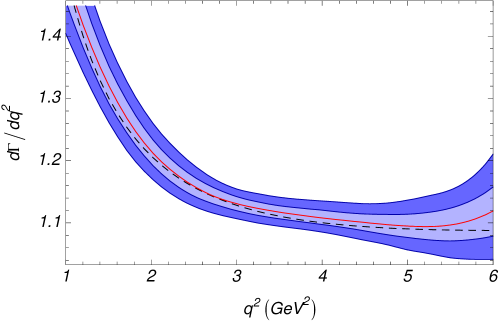
With the model above we can generate an ensemble of experiments corresponding to a given integrated luminosity. In each of these experiments we can use a general minimiser to find the spin value parametrisation that best corresponds to the data. Each fit has in total 27 parameters; 26 from the signal described above and a single parameter to describe the level of the simplified background model. From the ensemble of experiments, estimates of the experimental uncertainties can be made and any biases introduced can be studied. For each dataset, the extracted spin amplitude components were used to calculate the value of each angular observable as a function of q2superscript𝑞2q^{2}. In total we created an ensemble of 1000 experiments and will thus at a given value of q2superscript𝑞2q^{2} get 1000 different determinations of a given observable. By looking at the point where 33% and 47.5% of results lie within either side of the median of the results we can form asymmetric 1σ1𝜎1\sigma and 2σ2𝜎2\sigma errors. Connecting these at different q2superscript𝑞2q^{2} values gives us 1σ1𝜎1\sigma and 2σ2𝜎2\sigma bands for the experimental errors on the observable. An illustration of the method in Fig. 1 shows the experimental sensitivity to the width distribution relative to the normalisation point which was arbitrarily chosen as 3.5GeV2superscriptGeV2{\mathrm{\,Ge\kern-1.00006ptV^{2}}}. The inner and outer bands correspond to 1σ𝜎\sigma and 2σ𝜎\sigma experimental errors with statistics corresponding to a 10 fb1superscript fb1\mbox{\,fb}^{-1} dataset from LHCb. The dashed line is the theoretical input and the red line the central value of the ensemble experiments. The difference between these two lines is caused by limitations imposed by the second order polynomial assumption. As it is is well inside the 1σ𝜎\sigma band this is not problem.

Refer to caption
Figure 1: The experimental sensitivity to dΓdq2𝑑Γ𝑑superscript𝑞2\frac{d\Gamma}{dq^{2}} with the SM as input. The inner and outer bands correspond to 1σ𝜎\sigma and 2σ𝜎\sigma experimental errors with statistics corresponding to a 10 fb1superscript fb1\mbox{\,fb}^{-1} dataset from LHCb. The black dashed line is the theoretical input and the red solid line the central value of the ensemble experiments.

The experimental sensitivity to the observables introduced in Sec. 4.2 will be presented in Sec. 6 within the phenomenological analysis to allow for an easy comparison of experimental and theoretical errors.

5.3 Comparisons with fits to projections

The full angular fit gives access to angular observables not accessible in other ways. However, AFBsubscript𝐴FBA_{\mathrm{FB}}, AT(2)superscriptsubscript𝐴𝑇2A_{T}^{\left(2\right)}, FLsubscript𝐹LF_{\mathrm{L}} and Aimsubscript𝐴imA_{\mathrm{im}}111Aimsubscript𝐴imA_{\mathrm{im}} is defined as Aim=Im(ALAL)+Im(ARAR)|A0|2+|A|2+|A|2A_{\mathrm{im}}=\frac{\mathrm{Im}(A_{\perp L}A_{\|L}^{*})+\mathrm{Im}(A_{\perp R}A_{\|R}^{*})}{|A_{0}|^{2}+|A_{\perp}|^{2}+|A_{\|}|^{2}} and is included for completeness here. It is not of importance for the measurement of right handed currents. can be extracted from distributions in just a single angle after integration over the other 2 in Eq. (1):

dΓdϕ𝑑superscriptΓ𝑑italic-ϕ\displaystyle\frac{d\Gamma^{\prime}}{d\phi} =\displaystyle= Γ2π(1+12(1FL)AT(2)cos2ϕ+Aimsin2ϕ),superscriptΓ2𝜋1121subscript𝐹Lsuperscriptsubscript𝐴𝑇22italic-ϕsubscript𝐴im2italic-ϕ\displaystyle\frac{\Gamma^{\prime}}{2\pi}\left(1+\frac{1}{2}(1-F_{\mathrm{L}})A_{T}^{\left(2\right)}\cos 2\phi+A_{\mathrm{im}}\sin 2\phi\right), (27a)
dΓdθl𝑑superscriptΓ𝑑subscript𝜃𝑙\displaystyle\frac{d\Gamma^{\prime}}{d\theta_{l}} =\displaystyle= Γ(34FLsin2θl+38(1FL)(1+cos2θl)+AFBcosθl)sinθl,superscriptΓ34subscript𝐹Lsuperscript2subscript𝜃𝑙381subscript𝐹L1superscript2subscript𝜃𝑙subscript𝐴FBsubscript𝜃𝑙subscript𝜃𝑙\displaystyle\Gamma^{\prime}\left(\frac{3}{4}F_{\mathrm{L}}\sin^{2}\theta_{l}+\frac{3}{8}(1-F_{\mathrm{L}})(1+\cos^{2}\theta_{l})+A_{\mathrm{FB}}\cos\theta_{l}\right)\sin\theta_{l}\,, (27b)
dΓdθK𝑑superscriptΓ𝑑subscript𝜃𝐾\displaystyle\frac{d\Gamma^{\prime}}{d\theta_{K}} =\displaystyle= 3Γ4sinθK(2FLcos2θK+(1FL)sin2θK),3superscriptΓ4subscript𝜃𝐾2subscript𝐹Lsuperscript2subscript𝜃𝐾1subscript𝐹Lsuperscript2subscript𝜃𝐾\displaystyle\frac{3\Gamma^{\prime}}{4}\sin\theta_{K}\left(2F_{\mathrm{L}}\cos^{2}\theta_{K}+(1-F_{\mathrm{L}})\sin^{2}\theta_{K}\right), (27c)

where Γ=b+4csuperscriptΓ𝑏4𝑐\Gamma^{\prime}=b+4c. This method was investigated for LHCb in [12]. The observables appear linearly in the expressions so the fits can be performed on data binned in q2superscript𝑞2q^{2}. The value extracted from these fits is then a dΓdq2𝑑Γ𝑑superscript𝑞2\frac{d\Gamma}{dq^{2}} weighted average of each parameter.

The full angular model described in Sec. 5.2 was used to generate data sets which were then fit simultaneously using the distributions in Eq. (27). The treatment of background and the mB,Kπsubscript𝑚𝐵𝐾𝜋m_{B,K\pi} distributions were the same as in the full angular model. For a direct comparison between this method and the full angular fit, the q2superscript𝑞2q^{2} dependent values of the observables were averaged using a weighted mean,

AT(i)=qmin2qmax2dΓdq2AT(i)(q2)qmin2qmax2dΓdq2.superscriptsubscript𝐴𝑇𝑖superscriptsubscriptsubscriptsuperscript𝑞2subscriptsuperscript𝑞2𝑑Γ𝑑superscript𝑞2superscriptsubscript𝐴𝑇𝑖superscript𝑞2superscriptsubscriptsubscriptsuperscript𝑞2subscriptsuperscript𝑞2𝑑Γ𝑑superscript𝑞2A_{T}^{\left(i\right)}=\frac{\int_{q^{2}_{\min}}^{q^{2}_{\max}}\frac{d\Gamma}{dq^{2}}A_{T}^{\left(i\right)}(q^{2})}{\int_{q^{2}_{\min}}^{q^{2}_{\max}}\frac{d\Gamma}{dq^{2}}}\,. (28)

The central values produced for the full angular approach in this case show some small biases due to the breakdown of the polynomial ansatz at the edges of the q2superscript𝑞2q^{2} distribution, however this is still well below the statistical error expected with 10 fb1superscript fb1\mbox{\,fb}^{-1} of data from LHCb. The power of the full angular fit is striking for AT(2)superscriptsubscript𝐴𝑇2A_{T}^{\left(2\right)} where the resolution is above a factor 2 better compared to fitting the projections. This can easily be understood in terms of the (1FL)1subscript𝐹L(1-F_{\mathrm{L}}) factor in Eq. (27a), where FLsubscript𝐹LF_{\mathrm{L}} is large in the SM.

For all the observables where a comparison can be made, we see that the full angular fit provides improvements in the resolution of between 15% and 60%.

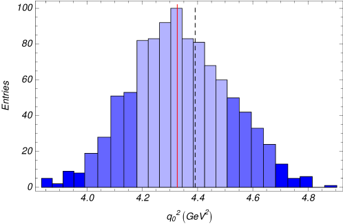
In the full angular fit we can calculate the position of the zero crossing for the forward-backward asymmetry, q02subscriptsuperscript𝑞20q^{2}_{0}. We illustrate the distribution of results obtained from the ensemble of datasets in Fig. 2 where a resolution, assuming the SM as input, of 0.17GeV2superscriptGeV2{\mathrm{\,Ge\kern-1.00006ptV^{2}}} is obtained. Alternatively we can perform the simpler task of binning the data in 1GeV2superscriptGeV2{\mathrm{\,Ge\kern-1.00006ptV^{2}}} bins and then in each bin perform simultaneous fits to the three angular projections. The value of AFBsubscript𝐴FBA_{\mathrm{FB}} is extracted by performing a straight line fit in the range 26GeV226superscriptGeV22-6{\mathrm{\,Ge\kern-1.00006ptV^{2}}} to the AFBsubscript𝐴FBA_{\mathrm{FB}} values found in each q2superscript𝑞2q^{2} bin. This gives us, with exactly the same assumptions for how background and acceptance are treated, a resolution of 0.24GeV2superscriptGeV2{\mathrm{\,Ge\kern-1.00006ptV^{2}}}. So also in this case we see an improvement of 30% in the statistical power by performing a full angular fit.
Refer to caption
Figure 2: The distribution in the determination of the zero crossing of AFBsubscript𝐴FBA_{\mathrm{FB}} from an ensemble of datasets created from the toy Monte Carlo model with statistics corresponding to 10 fb1superscript fb1\mbox{\,fb}^{-1} at LHCb. The edge of the inner (light blue) and middle (medium blue) regions correspond to 1σ𝜎\sigma and 2σ𝜎\sigma experimental errors. The solid (red) line is the median of the fitted values and the dashed (black) line is the input value from the SM theory predictions. From the figure we see a resolution of 0.17GeV2superscriptGeV2{\mathrm{\,Ge\kern-1.00006ptV^{2}}}.

The comparisons made here demonstrate that there is significant advantage in performing the full angular fit once the data sets are large enough. Using the simplified model described here it is possible to use this approach even with a smaller 2 fb1superscript fb1\mbox{\,fb}^{-1} data set. In reality, detector effects not accounted for such as angular acceptance will complicate the process and a proper full angular analysis may not be possible with data sets this small. However, we have shown that with the signal and background statistics at LHCb a full angular analysis is possible once the detector effects have been properly understood.

6 Phenomenological analysis

In this section we present our phenomenological analysis of the old and new observables in the SM and in extensions of the SM with new right-handed currents. The latter can be done in a model independent way by introducing the chiral partners of the SM Wilson coefficients 𝒞7(eff)superscriptsubscript𝒞7eff\mathcal{C}_{7}^{\mathrm{(eff)}}, 𝒞9(eff)superscriptsubscript𝒞9eff\mathcal{C}_{9}^{\mathrm{(eff)}}, and 𝒞10subscript𝒞10\mathcal{C}_{10}222We note here that the impact of 𝒞9(eff)superscriptsubscript𝒞9eff\mathcal{C}_{9}^{\mathrm{(eff)}} and 𝒞10subscript𝒞10\mathcal{C}_{10} and their chiral partners is rather small compared with 𝒞7(eff)\mathcal{C}_{7}^{{}^{\prime}\mathrm{(eff)}} in the low-q2superscript𝑞2q^{2} region, due to the 2 m^b/s^subscript^𝑚𝑏^𝑠{\hat{m}_{b}}/{\hat{s}} factor in the matrix element and the experimental constraints from the inclusive decay BXs+𝐵subscript𝑋𝑠superscriptsuperscriptB\rightarrow X_{s}\ell^{+}\ell^{-}.. This general new-physics scenario can be realized for example via gluino-mediated FCNC in the general R-parity conserving MSSM.

6.1 Preliminaries

Our analysis is based on the numerical input as summarized in Table 1. Regarding the form factor value we follow Ref. [35] and use the value fixed by experimental data.

Table 1: Summary of input parameters and estimated uncertainties.

mBsubscript𝑚𝐵\!\!m_{B} 5.27950±0.00033GeVplus-or-minus5.279500.00033GeV5.27950\pm 0.00033\,{\rm GeV} λ𝜆\lambda 0.2262±0.0014plus-or-minus0.22620.00140.2262\pm 0.0014
mKsubscript𝑚𝐾m_{K} 0.896±0.040GeVplus-or-minus0.8960.040GeV0.896\pm 0.040\,{\rm GeV} A𝐴A 0.815±0.013plus-or-minus0.8150.0130.815\pm 0.013
MWsubscript𝑀𝑊M_{W} 80.403±0.029GeVplus-or-minus80.4030.029GeV80.403\pm 0.029\,{\rm GeV} ρ¯¯𝜌\bar{\rho} 0.235±0.031plus-or-minus0.2350.0310.235\pm 0.031
MZsubscript𝑀𝑍M_{Z} 91.1876±0.0021GeVplus-or-minus91.18760.0021GeV91.1876\pm 0.0021\,{\rm GeV} η¯¯𝜂\bar{\eta} 0.349±0.020plus-or-minus0.3490.0200.349\pm 0.020
m^t(m^t)subscript^𝑚𝑡subscript^𝑚𝑡\!\!\hat{m}_{t}(\hat{m}_{t}) 167±5plus-or-minus1675167\pm 5 GeV ΛQCD(nf=5)superscriptsubscriptΛQCDsubscript𝑛𝑓5\mathchar 28931\relax_{\rm QCD}^{(n_{f}=5)} 220±40MeVplus-or-minus22040MeV220\pm 40\,{\rm MeV}
mb,PS(2GeV)subscript𝑚𝑏PS2GeVm_{b,\rm PS}(2\,\mbox{GeV}) 4.6±0.1plus-or-minus4.60.14.6\pm 0.1 GeV αs(MZ)subscript𝛼𝑠subscript𝑀𝑍\alpha_{s}(M_{Z}) 0.1176±0.0002plus-or-minus0.11760.00020.1176\pm 0.0002
mcsubscript𝑚𝑐m_{c} 1.5±0.2plus-or-minus1.50.21.5\pm 0.2 GeV αemsubscript𝛼em\alpha_{\rm em} 1/13711371/137
fBsubscript𝑓𝐵\!\!f_{B} 200±30plus-or-minus20030200\pm 30 MeV a1(K),a_{1}(K^{*})_{\perp,\,\parallel} 0.10±0.07plus-or-minus0.100.070.10\pm 0.07
fK,subscript𝑓superscript𝐾perpendicular-tof_{K^{*},\perp} 175±25plus-or-minus17525175\pm 25 MeV a2(K)subscript𝑎2subscriptsuperscript𝐾perpendicular-toa_{2}(K^{*})_{\perp} 0.13±0.08plus-or-minus0.130.080.13\pm 0.08
fK,f_{K^{*},\parallel} 217±5plus-or-minus2175217\pm 5 MeV a2(K)subscript𝑎2subscriptsuperscript𝐾parallel-toa_{2}(K^{*})_{\parallel} 0.09±0.05plus-or-minus0.090.050.09\pm 0.05
mBξK,(0)/(2mK)\!\!m_{B}\,\xi_{K^{*},\parallel}(0)/(2m_{K^{*}}) 0.47±0.09plus-or-minus0.470.090.47\pm 0.09 λB,+(1.5GeV)subscript𝜆𝐵1.5GeV\lambda_{B,+}(1.5{\rm GeV}) 0.485±0.115GeVplus-or-minus0.4850.115GeV0.485\pm 0.115\,{\rm GeV}
ξK,(0)subscript𝜉superscript𝐾perpendicular-to0\xi_{K^{*},\perp}(0) 0.26±0.02plus-or-minus0.260.020.26\pm 0.02

Moreover, we introduce four representative benchmark points of supersymmetry with non-minimal flavour violation in the down squark sector which were already used in Ref. [20]. The most important flavour diagonal parameters are fixed as follows: tanβ=5𝛽5\tan\beta=5, μ=M1=M2=MH+=mu~R=1TeV𝜇subscript𝑀1subscript𝑀2subscript𝑀superscript𝐻subscript𝑚subscript~𝑢𝑅1TeV\mu=M_{1}=M_{2}=M_{H^{+}}=m_{\tilde{u}_{R}}=1\mathrm{\,Te\kern-1.00006ptV}. Note that we choose a low value for tanβ𝛽\tan\beta; this shows that we do not need to rely on a large-tanβ𝛽\tan\beta to see an effect, and ensures automatic fulfilment of the constraint coming from Bsμ+μsubscript𝐵𝑠superscript𝜇superscript𝜇B_{s}\rightarrow\mu^{+}\mu^{-}. Furthermore, we make the assumption that all the entries in mu,LR2subscriptsuperscript𝑚2𝑢𝐿𝑅m^{2}_{u,LR} and md,LR2subscriptsuperscript𝑚2𝑑𝐿𝑅m^{2}_{d,LR} vanish, with the exception of the one that corresponds to (δLRd)32subscriptsuperscriptsubscript𝛿𝐿𝑅𝑑32\left(\delta_{LR}^{d}\right)_{32}. The remaining parameters of the four benchmark points correspond to two different scenarios and are fixed as follows333We follow here the conventions of Ref. [36]:

  • Scenario A: mg~=1TeVsubscript𝑚~𝑔1TeVm_{\tilde{g}}=1\mathrm{\,Te\kern-1.00006ptV} and md~[200,1000]GeVsubscript𝑚~𝑑2001000GeVm_{\tilde{d}}\in[200,1000]\mathrm{\,Ge\kern-1.00006ptV}. The only non-zero mass insertion is varied between 0.1(δLRd)320.10.1subscriptsuperscriptsubscript𝛿𝐿𝑅𝑑320.1-0.1\leq\left(\delta_{LR}^{d}\right)_{32}\leq 0.1. For all parameter sets the compatibility with other B𝐵B physics constraints, the electroweak constraints, constraints from particle searches, and also with the vacuum stability bounds is verified [20]. The curves denoted by (a) and (b) correspond respectively to mg~/md~=2.5subscript𝑚~𝑔subscript𝑚~𝑑2.5m_{\tilde{g}}/m_{\tilde{d}}=2.5, (δLRd)32=0.016subscriptsuperscriptsubscript𝛿𝐿𝑅𝑑320.016\left(\delta_{LR}^{d}\right)_{32}=0.016 and mg~/md~=4subscript𝑚~𝑔subscript𝑚~𝑑4m_{\tilde{g}}/m_{\tilde{d}}=4, (δLRd)32=0.036subscriptsuperscriptsubscript𝛿𝐿𝑅𝑑320.036\left(\delta_{LR}^{d}\right)_{32}=0.036. We will refer to this case as the large-gluino and positive mass insertion scenario. In terms of the effective Wilson coefficients at mbsubscript𝑚𝑏m_{b}, model (a) corresponds to (𝒞7(eff),𝒞7(eff))=(0.32,0.16)(\mathcal{C}_{7}^{\mathrm{(eff)}},\mathcal{C}_{7}^{{}^{\prime}\mathrm{(eff)}})=(-0.32,0.16) and (b) to (0.32,0.24)0.320.24(-0.32,0.24). This should be compared to the SM value of (𝒞7(eff),𝒞7(eff))=(0.31,0.00)(\mathcal{C}_{7}^{\mathrm{(eff)}},\mathcal{C}_{7}^{{}^{\prime}\mathrm{(eff)}})=(-0.31,0.00).

  • Scenario B: md~=1TeVsubscript𝑚~𝑑1TeVm_{\tilde{d}}=1\mathrm{\,Te\kern-1.00006ptV} and mg~[200,800]GeVsubscript𝑚~𝑔200800GeVm_{\tilde{g}}\in[200,800]\mathrm{\,Ge\kern-1.00006ptV}. The mass insertion is varied in the same range as Scenario A. The curves denoted by (c) and (d) correspond respectively to mg~/md~=0.7subscript𝑚~𝑔subscript𝑚~𝑑0.7m_{\tilde{g}}/m_{\tilde{d}}=0.7, (δLRd)32=0.004subscriptsuperscriptsubscript𝛿𝐿𝑅𝑑320.004\left(\delta_{LR}^{d}\right)_{32}=-0.004 and mg~/md~=0.6subscript𝑚~𝑔subscript𝑚~𝑑0.6m_{\tilde{g}}/m_{\tilde{d}}=0.6, (δLRd)32=0.006subscriptsuperscriptsubscript𝛿𝐿𝑅𝑑320.006\left(\delta_{LR}^{d}\right)_{32}=-0.006. We will refer to this case as the low-gluino mass (although large squark mass would be more appropriate) and negative mass insertion scenario. In this case the corresponding effective Wilson coefficients are (𝒞7(eff),𝒞7(eff))=(0.32,0.08)(\mathcal{C}_{7}^{\mathrm{(eff)}},\mathcal{C}_{7}^{{}^{\prime}\mathrm{(eff)}})=(-0.32,-0.08) for (c) and (0.32,0.13)0.320.13(-0.32,-0.13) for (d).

Notice that we have changed curve (c) with respect to Ref. [20] reducing its corresponding mass insertion to avoid any conflict with vacuum stability or colour breaking constraints [37].

Finally, we emphasize again that the validity of our theoretical predictions is restricted to the kinematic region in which the energy of the Ksuperscript𝐾K^{*} is of the order of the heavy quark mass. So we restrict our analysis to the low-q2superscript𝑞2q^{2} region from 1GeV2superscriptGeV2{\mathrm{\,Ge\kern-1.00006ptV^{2}}} to 6GeV2superscriptGeV2{\mathrm{\,Ge\kern-1.00006ptV^{2}}}. In the region below 1GeV2superscriptGeV2{\mathrm{\,Ge\kern-1.00006ptV^{2}}} the QCDf/SCET results are questioned by the presence of very light resonances.

6.2 Results

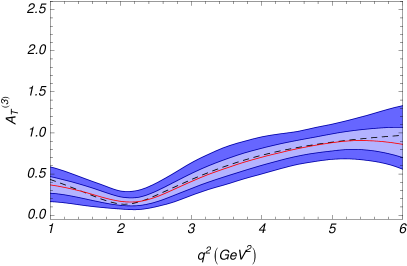
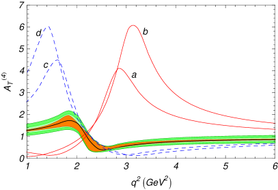
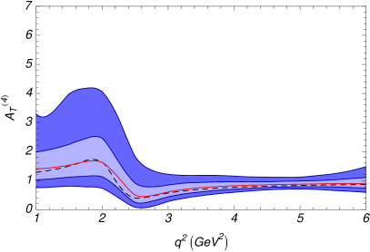
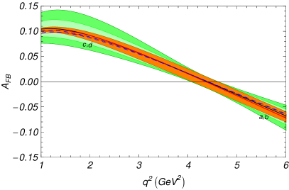
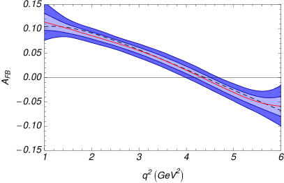
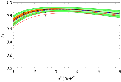
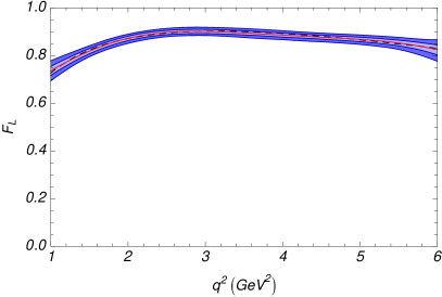
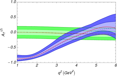
We present our results on the observables AT(2)superscriptsubscript𝐴𝑇2A_{T}^{\left(2\right)}, AT(3)superscriptsubscript𝐴𝑇3A_{T}^{\left(3\right)}, AT(4)superscriptsubscript𝐴𝑇4A_{T}^{\left(4\right)}, AFBsubscript𝐴FBA_{\mathrm{FB}} and FLsubscript𝐹𝐿F_{L} in the Figs. 37 (for definitions see Sec. 4). For all the observables we plot the theoretical sensitivity on the left hand side of each Figure.

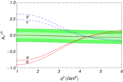
  • The thin dark line is the central NLO result for the SM and the narrow inner dark (orange) band that surrounds it corresponds to the NLO SM uncertainties due to both input parameters and perturbative scale dependence. Light grey (green) bands are the estimated Λ/mb±5%plus-or-minusΛsubscript𝑚𝑏percent5\mathchar 28931\relax/m_{b}\pm 5\% corrections for each spin amplitude (as given in Eq. 13) while darker grey (green) ones are the more conservative Λ/mb±10%plus-or-minusΛsubscript𝑚𝑏percent10\mathchar 28931\relax/m_{b}\pm 10\% corrections. The curves labelled (a)–(d) correspond to the four different benchmark points in the MSSM introduced above.

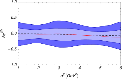
  • The experimental sensitivity for a dataset corresponding to 10 fb1superscript fb1\mbox{\,fb}^{-1} of LHCb data is given in each figure on the right hand side. Here the solid (red) line shows the median extracted from the fit to the ensemble of data and the dashed (black) line shows the theoretical input distribution. The inner and outer bands correspond to 1σ𝜎\sigma and 2σ𝜎\sigma experimental errors.

Refer to caption
Refer to caption
Figure 3: For AT(2)superscriptsubscript𝐴𝑇2A_{T}^{\left(2\right)} we compare the theoretical errors (left) with the experimental errors (right) as a function of the squared dimuon mass. For the theory, the narrow inner dark (orange) bands correspond to the NLO result for the SM including all uncertainties (except for Λ/mbΛsubscript𝑚𝑏\mathchar 28931\relax/m_{b}) as explained in the text. Light grey (green) bands include the estimated Λ/mbΛsubscript𝑚𝑏\mathchar 28931\relax/m_{b} uncertainty at a ±5%plus-or-minuspercent5\pm 5\% level and the external dark grey (green) bands correspond to a ±10%plus-or-minuspercent10\pm 10\% correction for each spin amplitude. The curves labelled (a)–(d) correspond to different SUSY scenarios as explained in the text. For the experimental aspects the inner and outer bands correspond to 1σ𝜎\sigma and 2σ𝜎\sigma statistical errors with a yield corresponding to a 10 fb1superscript fb1\mbox{\,fb}^{-1} dataset from LHCb.
Refer to caption
Refer to caption
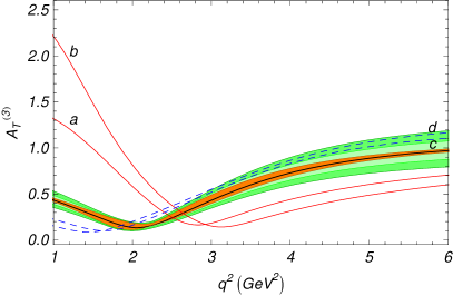
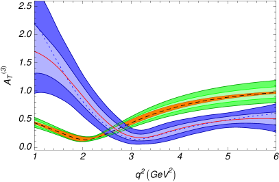
Figure 4: For the new observable AT(3)superscriptsubscript𝐴𝑇3A_{T}^{\left(3\right)} we compare the theoretical errors (left) with the experimental errors (right). See the caption of Fig. 3 for details.
Refer to caption
Refer to caption
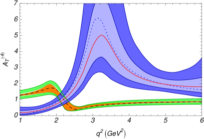
Figure 5: For the new observable AT(4)superscriptsubscript𝐴𝑇4A_{T}^{\left(4\right)} we compare the theoretical errors (left) with the experimental errors (right). See the caption of Fig. 3 for details.
Refer to caption
Refer to caption
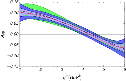
Figure 6: For AFBsubscript𝐴𝐹𝐵A_{FB} we compare the theoretical errors (left) with the experimental errors (right). See the caption of Fig. 3 for details.
Refer to caption
Refer to caption
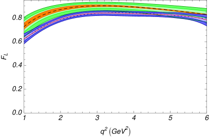
Figure 7: For FLsubscript𝐹𝐿F_{L} we compare the theoretical errors (left) with the experimental errors (right). See the caption of Fig. 3 for details.

Let us start with some concrete observations on the new observables AT(3)superscriptsubscript𝐴𝑇3A_{T}^{\left(3\right)} and AT(4)superscriptsubscript𝐴𝑇4A_{T}^{\left(4\right)}. They offer sensitivity to the longitudinal spin amplitude A0L,Rsubscript𝐴0𝐿𝑅A_{0L,R} in a controlled way compared to the old observables FLsubscript𝐹𝐿F_{L} and αKsuperscriptsubscript𝛼𝐾\alpha_{K}^{*}: the dependence on both the parallel and perpendicular soft form factors ξ(0)subscript𝜉0\xi_{\|}(0) and ξ(0)subscript𝜉perpendicular-to0\xi_{\perp}(0) cancels at LO. A residual of this dependence may appear at NLO, but as shown in Figs. 4 and 5, it is basically negligible. It is also remarkable that for AT(3)superscriptsubscript𝐴𝑇3A_{T}^{\left(3\right)} and AT(4)superscriptsubscript𝐴𝑇4A_{T}^{\left(4\right)} at low q2superscript𝑞2q^{2} the impact of this uncertainty is less important than the uncertainties due to input parameters and scale dependence.

The peaking structure in AT(4)superscriptsubscript𝐴𝑇4A_{T}^{\left(4\right)} as a function of q2superscript𝑞2q^{2} for the benchmark MSSM points is due to the different way 𝒞7(eff)\mathcal{C}_{7}^{{}^{\prime}\mathrm{(eff)}} enters numerator and denominator; the numerator has a positive slope in the region of the peak, while the denominator has a minimum at the same point. If one uses the simplified L0 expressions from Eqs. 1012 the denominator is exactly zero, generating an infinity at the point of the peak; however, once NLO QCDf is included the zero in the denominator is lifted and the result is a curve with a peak instead.

The new observables AT(3)superscriptsubscript𝐴𝑇3A_{T}^{\left(3\right)} and AT(4)superscriptsubscript𝐴𝑇4A_{T}^{\left(4\right)} also present a different sensitivity to 𝒞7(eff)\mathcal{C}_{7}^{{}^{\prime}\mathrm{(eff)}} via their dependence on A0L,Rsubscript𝐴0𝐿𝑅A_{0L,R} compared with AT(2)superscriptsubscript𝐴𝑇2A_{T}^{\left(2\right)}. This may allow for a particularly interesting cross check of the sensitivity to this chirality flipped operator 𝒪7superscriptsubscript𝒪7\mathcal{O}_{7}^{{}^{\prime}}; for instance, new contributions coming from tensor scalars and pseudo-scalars will behave differently among the set of observables.

Another remarkable point that comes clear when comparing the set of clean observables AT(2)superscriptsubscript𝐴𝑇2A_{T}^{\left(2\right)}, AT(3)superscriptsubscript𝐴𝑇3A_{T}^{\left(3\right)} and AT(4)superscriptsubscript𝐴𝑇4A_{T}^{\left(4\right)} versus the old observables like FLsubscript𝐹𝐿F_{L} concerns the potential discovery of NP, in particular of new right-handed currents. The new observables share the nice feature of AT(2)superscriptsubscript𝐴𝑇2A_{T}^{\left(2\right)} that there are large deviations from the SM curve from the ones of the four supersymmetric benchmark points. In case of AT(2)superscriptsubscript𝐴𝑇2A_{T}^{\left(2\right)} this is caused by the balance between the competing contributions of order 1/q21superscript𝑞21/q^{2} and 1/q41superscript𝑞41/q^{4} originating from the photon pole in the numerator and denominator of AT(2)superscriptsubscript𝐴𝑇2A_{T}^{\left(2\right)}, providing a strong sensitivity to 𝒞7(eff)\mathcal{C}_{7}^{{}^{\prime}\mathrm{(eff)}}. This sensitivity is near maximal around the 1GeV2superscriptGeV2{\mathrm{\,Ge\kern-1.00006ptV^{2}}} region precisely inside the theoretically well controlled area. A large deviation from the SM for AT(2)superscriptsubscript𝐴𝑇2A_{T}^{\left(2\right)}, AT(3)superscriptsubscript𝐴𝑇3A_{T}^{\left(3\right)} or AT(4)superscriptsubscript𝐴𝑇4A_{T}^{\left(4\right)} can thus show the presence of right-handed currents in a way that is not possible with FLsubscript𝐹𝐿F_{L} or AFBsubscript𝐴𝐹𝐵A_{FB}. In the latter cases the deviations from the SM prediction of the same four representative curves are marginal.

In the experimental plots we find a good agreement between the central values extracted from the fits and the theoretical input. Any deviations seen are small compared to the statistical uncertainties, however the weakness of the polynomial parametrisation, particularly at the extremes of the q2superscript𝑞2q^{2} range, can be seen. For much larger data sets this could be addressed by increasing the order of the polynomials used. The experimental resolution for FLsubscript𝐹𝐿F_{L} is very good but with the small deviations from the SM expected this is not helpful in the discovery of new right-handed currents. Comparing the theoretical and experimental figures for the other observables it can be seen that in particular AT(3)superscriptsubscript𝐴𝑇3A_{T}^{\left(3\right)} show great promise to distinguish between NP models.

To further explore the power of the observables we can imagine that nature corresponds to SUSY scenario (b). We create an ensemble of datasets from the toy Monte Carlo model assuming model (b) as input and compare the results to the SM prediction including the theoretical errors to get a feeling for how significantly different from the SM prediction the results are. The results of this are presented in Figs. 8-10: It can be seen that AT(2)superscriptsubscript𝐴𝑇2A_{T}^{\left(2\right)}, AT(3)superscriptsubscript𝐴𝑇3A_{T}^{\left(3\right)} and AT(4)superscriptsubscript𝐴𝑇4A_{T}^{\left(4\right)} all show a remarkable separation between the experimental error band and the SM prediction thus providing high sensitivity to NP. For the SUSY scenario (b) chosen here, the deviation for AFBsubscript𝐴FBA_{\mathrm{FB}} and FLsubscript𝐹𝐿F_{L} on the other hand is minor.

Refer to caption
Refer to caption
Figure 8: The experimental errors (blue, on top) assuming SUSY scenario (b) with large-gluino mass and positive mass insertion, is compared to the theoretical errors (green, below) assuming the SM. To the left for AT(2)superscriptsubscript𝐴𝑇2A_{T}^{\left(2\right)} and the right for AT(3)superscriptsubscript𝐴𝑇3A_{T}^{\left(3\right)}.
Refer to caption
Figure 9: The experimental errors (blue, on top) assuming SUSY scenario (b) with large-gluino mass and positive mass insertion, is compared to the theoretical errors (green, below) assuming the SM. Here the observable AT(4)superscriptsubscript𝐴𝑇4A_{T}^{\left(4\right)} is considered.
Refer to caption
Refer to caption
Figure 10: The experimental errors (blue, on top) assuming SUSY scenario (b) with large-gluino mass and positive mass insertion, is compared to the theoretical errors (green, below) assuming the SM. To the left for AFBsubscript𝐴FBA_{\mathrm{FB}} and the right for FLsubscript𝐹𝐿F_{L}.
Refer to caption
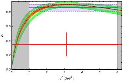
Figure 11: Weighted SM average over the bin q2[1GeV2,6GeV2]superscript𝑞21superscriptGeV26superscriptGeV2q^{2}\in[1{\mathrm{\,Ge\kern-1.00006ptV^{2}}},6{\mathrm{\,Ge\kern-1.00006ptV^{2}}}] and recent BABAR measurement using the extended bin q2[4mμ2,6.25GeV2]superscript𝑞24superscriptsubscript𝑚𝜇26.25superscriptGeV2q^{2}\in[4m_{\mu}^{2},6.25{\mathrm{\,Ge\kern-1.00006ptV^{2}}}] (shown in grey).

As mentioned in the introduction, the B𝐵B factories can already access some of the angular observables using the projection-fit method described in Sec. 5. For example, recently the BABAR collaboration announced the first measurement of the longitudinal polarisation in the low q2superscript𝑞2q^{2} region as an average over the bin q2[4mμ2,6.25GeV2]superscript𝑞24superscriptsubscript𝑚𝜇26.25superscriptGeV2q^{2}\in[4m_{\mu}^{2},6.25{\mathrm{\,Ge\kern-1.00006ptV^{2}}}] [8] (see Fig. 11):

FL(q2[4mμ2,6.25GeV2])=0.35±0.16stat±0.04syst.subscript𝐹𝐿superscript𝑞24superscriptsubscript𝑚𝜇26.25superscriptGeV2plus-or-minus0.35subscript0.16statsubscript0.04systF_{L}(q^{2}\in[4m_{\mu}^{2},6.25{\mathrm{\,Ge\kern-1.00006ptV^{2}}}])=0.35\pm 0.16_{\rm stat}\pm 0.04_{\rm syst}\,. (29)

However, as mentioned before, the spectrum below 1GeV2superscriptGeV2{\mathrm{\,Ge\kern-1.00006ptV^{2}}} is theoretically problematic; moreover the rate and also the polarisation FLsubscript𝐹𝐿F_{L} are changing dramatically around 1GeV2superscriptGeV2{\mathrm{\,Ge\kern-1.00006ptV^{2}}}. Therefore, we strongly recommend to use the standard bin from 1GeV2superscriptGeV2{\mathrm{\,Ge\kern-1.00006ptV^{2}}} to 6GeV2superscriptGeV2{\mathrm{\,Ge\kern-1.00006ptV^{2}}}. For future comparison we give here the theoretical average, weighted over the rate, using the bin, q2[1GeV2,6GeV2]superscript𝑞21superscriptGeV26superscriptGeV2q^{2}\in[1{\mathrm{\,Ge\kern-1.00006ptV^{2}}},6{\mathrm{\,Ge\kern-1.00006ptV^{2}}}], based on our results:

FL(q2[1GeV2,6GeV2])=0.86±0.05.subscript𝐹𝐿superscript𝑞21superscriptGeV26superscriptGeV2plus-or-minus0.860.05F_{L}(q^{2}\in[1{\mathrm{\,Ge\kern-1.00006ptV^{2}}},6{\mathrm{\,Ge\kern-1.00006ptV^{2}}}])=0.86\pm 0.05\,. (30)

and refer to Fig. 7 for the future experimental sensitivity of the LHCb experiment. In Fig. 11 we see the theoretical q2superscript𝑞2q^{2} distribution of FLsubscript𝐹LF_{\mathrm{L}} with the rate average overlaid.

Refer to caption
Refer to caption
Refer to caption
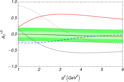
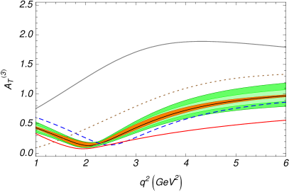
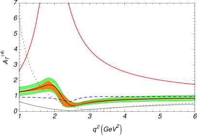
Figure 12: The distribution of AT(2)superscriptsubscript𝐴𝑇2A_{T}^{\left(2\right)}, AT(3)superscriptsubscript𝐴𝑇3A_{T}^{\left(3\right)} and AT(4)superscriptsubscript𝐴𝑇4A_{T}^{\left(4\right)} for four allowed combinations of 𝒞7(eff)superscriptsubscript𝒞7eff\mathcal{C}_{7}^{\mathrm{(eff)}} and 𝒞7(eff)\mathcal{C}_{7}^{{}^{\prime}\mathrm{(eff)}} following the model independent analysis of [21]. The bands correspond to the SM and the theoretical uncertainty as described in Fig 3. The solid heavy (red) line corresponds to (𝒞7(eff),𝒞7(eff))=(0.04,0.31)(\mathcal{C}_{7}^{\mathrm{(eff)}},\mathcal{C}_{7}^{{}^{\prime}\mathrm{(eff)}})=(0.04,0.31), the solid light (grey) line (0.03,0.32)0.030.32(-0.03,-0.32), the dashed (blue) line (0.35,0.05)0.350.05(-0.35,0.05), and the dotted (brown) line (0.24,0.19)0.240.19(-0.24,-0.19). Combining measurements in all three asymmetries will provide clear distinction between the different allowed regions.

Rather than using the benchmark supersymmetry points for the illustration of the power of the observables, one can also look at it from a model independent point of view. For this we have taken four illustrative points from Fig. 2 in [21] which are all allowed given the constraints from present measurements of bs𝑏𝑠b\rightarrow s transitions. In Fig. 12 the effect can be seen on AT(2)superscriptsubscript𝐴𝑇2A_{T}^{\left(2\right)}, AT(3)superscriptsubscript𝐴𝑇3A_{T}^{\left(3\right)} and AT(4)superscriptsubscript𝐴𝑇4A_{T}^{\left(4\right)}. It is clear that the combination of all observables will act as a way to reduce the allowed regions for a model independent analysis.
Refer to caption
Refer to caption
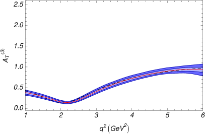
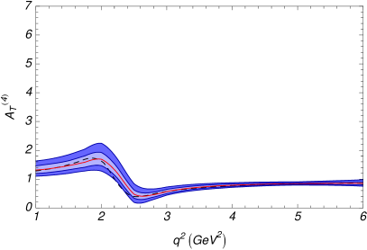
Figure 13: The experimental errors in AT(3)superscriptsubscript𝐴𝑇3A_{T}^{\left(3\right)} (right) and AT(4)superscriptsubscript𝐴𝑇4A_{T}^{\left(4\right)} left assuming the SM for statistics equivalent to 100 fb1superscript fb1\mbox{\,fb}^{-1} at the end of an upgrade to LHCb.

Finally we might ask what happens if we consider the situation with 100 fb1superscript fb1\mbox{\,fb}^{-1} of experimental data corresponding to the full dataset from an upgrade to LHCb. We assume the same performance of the experiment so simply scale the statistics by a factor 10 compared to the 10 fb1superscript fb1\mbox{\,fb}^{-1} study. The experimental errors are shown in Fig. 13 and are in general just a factor 1010\sqrt{10} smaller as expected. Comparing to Figs. 4 and 5 it can be seen that the Λ/mbΛsubscript𝑚𝑏\mathchar 28931\relax/m_{b} uncertainties will dominate unless progress is made on the theoretical side.

7 Summary

We have constructed two new observables AT(3)superscriptsubscript𝐴𝑇3A_{T}^{\left(3\right)} and AT(4)superscriptsubscript𝐴𝑇4A_{T}^{\left(4\right)} out of the Ksuperscript𝐾K^{*} spin amplitudes of the B¯dK¯μ+0μsubscript¯𝐵𝑑¯𝐾superscriptsuperscript𝜇absent0superscript𝜇\kern 3.00003pt\overline{\kern-2.40005ptB}_{d}\rightarrow\kern 1.99997pt\overline{\kern-1.99997ptK}{}^{*0}\mu^{+}\mu^{-} decay, that fulfil the criteria of being theoretically clean and can be experimentally extracted from the angular distribution of this decay with good precision. We have shown how to design the new observables for a specific kind of NP operator within the model independent analysis using the effective field theory approach.

We have presented a complete calculation of all observables in QCD factorization and have made the impact of unknown Λ/mbΛsubscript𝑚𝑏\mathchar 28931\relax/m_{b} corrections to the various observables explicit. Subsequently, we demonstrated the high sensitivity of AT(2)superscriptsubscript𝐴𝑇2A_{T}^{\left(2\right)}, AT(3)superscriptsubscript𝐴𝑇3A_{T}^{\left(3\right)} and AT(4)superscriptsubscript𝐴𝑇4A_{T}^{\left(4\right)} to right handed currents. Clearly theoretical progress on the Λ/mbΛsubscript𝑚𝑏\mathchar 28931\relax/m_{b} corrections would enhance that sensitivity significantly and would be desirable in view of an upgrade of the LHCb experiment.

The new observables AT(3)superscriptsubscript𝐴𝑇3A_{T}^{\left(3\right)} and AT(4)superscriptsubscript𝐴𝑇4A_{T}^{\left(4\right)} exhibit the important property of presenting a direct sensitivity to the longitudinal spin amplitude, while reducing at maximum the sensitivity to the poorly known longitudinal soft form factors within the whole low dilepton mass spectrum. Previously defined FLsubscript𝐹𝐿F_{L} or AFBsubscript𝐴FBA_{\mathrm{FB}} does not exhibit this behaviour. This same idea was behind the construction of AT(2)superscriptsubscript𝐴𝑇2A_{T}^{\left(2\right)} using the transverse amplitudes.

The combination of the three observables offer a full view of the sensitivity to NP of the three spin amplitudes with a good control of hadronic uncertainties.

Using a toy Monte Carlo approach we have estimated the statistical uncertainty of all observables for statistics corresponding to LHCb and also for Super-LHCb. The model performs a fit to the full angular and q2superscript𝑞2q^{2} distribution. AT(3)superscriptsubscript𝐴𝑇3A_{T}^{\left(3\right)} and AT(4)superscriptsubscript𝐴𝑇4A_{T}^{\left(4\right)} require a full angular fit and for AT(2)superscriptsubscript𝐴𝑇2A_{T}^{\left(2\right)} we have demonstrated that the resolution improves by more than a factor 2 compared to extracting AT(2)superscriptsubscript𝐴𝑇2A_{T}^{\left(2\right)} from angular projection. The experimental errors are such that measuring these new observables will be a powerful way to detect the presence of right handed currents. For the well known measurement of the zero point of the forward-backward asymmetry we see an improvement of 30% in the resolution from a full angular fit compared to fitting the angular projections.

Finally we have shown that the previously discussed angular distribution AT(1)superscriptsubscript𝐴𝑇1A_{T}^{\left(1\right)} cannot be measured at either LHCb or at a Super-B𝐵B factory.

Acknowledgments.
We thank Martin Beneke for detailed discussions on the forward-backward asymmetry. JM acknowledges financial support from FPA2005-02211, 2005-SGR-00994 and the RyC programme, MR from the Universitat Autonoma de Barcelona, and UE and WR from the Science and Technology Facilities Council (STFC). TH acknowledges support of the European network Heptools.

Appendix A Kinematics

Assuming the Ksuperscript𝐾K^{*} to be on the mass shell, the decay B0¯K¯0(Kπ+)+\bar{B^{0}}\rightarrow\bar{K}^{*0}(\rightarrow K^{-}\pi^{+})\ell^{+}\ell^{-} is completely described by four independent kinematic variables; namely, the lepton-pair invariant mass, q2superscript𝑞2q^{2}, and the three angles θlsubscript𝜃𝑙\theta_{l}, θKsubscript𝜃superscript𝐾\theta_{K^{*}}, ϕitalic-ϕ\phi as illustrated in Fig. 14. The sign of the angles for the B¯dsubscript¯𝐵𝑑\overline{\kern-2.40005ptB}_{d} decay shows great variation in the literature. Therefore we present here the most explicit definition of our conventions.

Refer to caption
Figure 14: Definition of kinematic variables in the decay B¯dK¯μ+0μsubscript¯𝐵𝑑¯𝐾superscriptsuperscript𝜇absent0superscript𝜇\kern 3.00003pt\overline{\kern-2.40005ptB}_{d}\rightarrow\kern 1.99997pt\overline{\kern-1.99997ptK}{}^{*0}\mu^{+}\mu^{-}: The z𝑧z-axis is the direction in which the B𝐵B meson flies in the rest frame of the μ+μsuperscript𝜇superscript𝜇\mu^{+}\mu^{-}. θlsubscript𝜃𝑙\theta_{l} is the angle between the μsuperscript𝜇\mu^{-} and the z𝑧z-axis in the μ+μsuperscript𝜇superscript𝜇\mu^{+}\mu^{-} rest frame, θKsubscript𝜃𝐾\theta_{K} is the angle between the Ksuperscript𝐾K^{-} and the z𝑧z-axis in the K¯\kern 1.99997pt\overline{\kern-1.99997ptK}{}^{*} rest frame, and ϕitalic-ϕ\phi is the angle between the normals to the μ+μsuperscript𝜇superscript𝜇\mu^{+}\mu^{-} and Kπ𝐾𝜋K\pi decay planes in the B𝐵B rest frame.

Here 𝐩𝐩\mathrm{\mathbf{p}} denote three momentum vectors in the B¯dsubscript¯𝐵𝑑\overline{\kern-2.40005ptB}_{d} rest frame, 𝐪𝐪\mathrm{\mathbf{q}} the same in the di-muon rest frame, and 𝐫𝐫\mathrm{\mathbf{r}} in the K¯0\kern 1.99997pt\overline{\kern-1.99997ptK}{}^{*0} rest frame, the z𝑧z-axis is defined as as the direction of the K¯0\kern 1.99997pt\overline{\kern-1.99997ptK}{}^{*0} in the B¯dsubscript¯𝐵𝑑\overline{\kern-2.40005ptB}_{d} rest frame. Three unit vectors are given in the following way: the first one is in the direction of the z𝑧z-axis where the θ𝜃\theta angles are measured with respect to, and the other two are perpendicular to the di-muon and K¯0\kern 1.99997pt\overline{\kern-1.99997ptK}{}^{*0} decay planes.

𝐞z=𝐩K+𝐩π+|𝐩K+𝐩π+|,𝐞l=𝐩μ×𝐩μ+|𝐩μ×𝐩μ+|,𝐞K=𝐩K×𝐩π+|𝐩K×𝐩π+|.formulae-sequencesubscript𝐞𝑧subscript𝐩superscript𝐾subscript𝐩superscript𝜋subscript𝐩superscript𝐾subscript𝐩superscript𝜋formulae-sequencesubscript𝐞𝑙subscript𝐩superscript𝜇subscript𝐩superscript𝜇subscript𝐩superscript𝜇subscript𝐩superscript𝜇subscript𝐞𝐾subscript𝐩superscript𝐾subscript𝐩superscript𝜋subscript𝐩superscript𝐾subscript𝐩superscript𝜋\mathrm{\mathbf{e}}_{z}=\frac{\mathrm{\mathbf{p}}_{K^{-}}+\mathrm{\mathbf{p}}_{\pi^{+}}}{|\mathrm{\mathbf{p}}_{K^{-}}+\mathrm{\mathbf{p}}_{\pi^{+}}|}\,,\qquad\mathrm{\mathbf{e}}_{l}=\frac{\mathrm{\mathbf{p}}_{\mu^{-}}\times\mathrm{\mathbf{p}}_{\mu^{+}}}{|\mathrm{\mathbf{p}}_{\mu^{-}}\times\mathrm{\mathbf{p}}_{\mu^{+}}|}\,,\qquad\mathrm{\mathbf{e}}_{K}=\frac{\mathrm{\mathbf{p}}_{K^{-}}\times\mathrm{\mathbf{p}}_{\pi^{+}}}{|\mathrm{\mathbf{p}}_{K^{-}}\times\mathrm{\mathbf{p}}_{\pi^{+}}|}\,. (31)

It follows for the B¯dsubscript¯𝐵𝑑\overline{\kern-2.40005ptB}_{d}

cosθl=𝐪μ𝐞z|𝐪μ|,cosθK=𝐫K𝐞z|𝐫K|formulae-sequencesubscript𝜃𝑙subscript𝐪superscript𝜇subscript𝐞𝑧subscript𝐪superscript𝜇subscript𝜃𝐾subscript𝐫superscript𝐾subscript𝐞𝑧subscript𝐫superscript𝐾\cos\theta_{l}=\frac{\mathrm{\mathbf{q}}_{\mu^{-}}\cdot\mathrm{\mathbf{e}}_{z}}{|\mathrm{\mathbf{q}}_{\mu^{-}}|}\,,\qquad\cos\theta_{K}=\frac{\mathrm{\mathbf{r}}_{K^{-}}\cdot\mathrm{\mathbf{e}}_{z}}{|\mathrm{\mathbf{r}}_{K^{-}}|} (32)

and

sinϕ=(𝐞l×𝐞K)𝐞z,cosϕ=𝐞K𝐞l.formulae-sequenceitalic-ϕsubscript𝐞𝑙subscript𝐞𝐾subscript𝐞𝑧italic-ϕsubscript𝐞𝐾subscript𝐞𝑙\sin\phi=(\mathrm{\mathbf{e}}_{l}\times\mathrm{\mathbf{e}}_{K})\cdot\mathrm{\mathbf{e}}_{z}\,,\qquad\cos\phi=\mathrm{\mathbf{e}}_{K}\cdot\mathrm{\mathbf{e}}_{l}\,. (33)

The angles are defined in the intervals

1cosθl1,1cosθK1,πϕ<π,formulae-sequence1subscript𝜃𝑙11subscript𝜃𝐾1𝜋italic-ϕ𝜋-1\leqslant\cos\theta_{l}\leqslant 1\,,\qquad-1\leqslant\cos\theta_{K}\leqslant 1\,,\qquad-\pi\leqslant\phi<\pi\,, (34)

where in particular it should be noted that the ϕitalic-ϕ\phi angle is signed.

In words, for the B¯dsubscript¯𝐵𝑑\overline{\kern-2.40005ptB}_{d} the angle θlsubscript𝜃𝑙\theta_{l} is measured as the angle between the μsuperscript𝜇\mu^{-} and the z𝑧z-axis in the dimuon rest frame. As the B¯dsubscript¯𝐵𝑑\overline{\kern-2.40005ptB}_{d} flies in the direction of the z𝑧z-axis in the dimuon rest frame this is equivalent to measuring θlsubscript𝜃𝑙\theta_{l} as the angle between the muon and the B¯dsubscript¯𝐵𝑑\overline{\kern-2.40005ptB}_{d} in the di-muon rest frame. The angle θKsubscript𝜃𝐾\theta_{K} is measured as the angle between the kaon and the z𝑧z-axis measured in the K¯0\kern 1.99997pt\overline{\kern-1.99997ptK}{}^{*0} rest frame. Finally ϕitalic-ϕ\phi is the angle between the normals to the planes defined by the Kπ𝐾𝜋K\pi system and the μ+μsuperscript𝜇superscript𝜇\mu^{+}\mu^{-} system in the rest frame of the B¯dsubscript¯𝐵𝑑\overline{\kern-2.40005ptB}_{d} meson.

Appendix B Theoretical framework

The coefficient functions Iisubscript𝐼𝑖I_{i} in the differential decay rate are given in terms of the Ksuperscript𝐾K^{*} spin amplitudes (see Eq. (3)) discussed in Sec. 3. The theoretical expressions of those spin amplitudes can be derived using the following standard steps:

  • The effective Hamiltonian describing the quark transition bs+𝑏𝑠superscriptsuperscriptb\rightarrow s\ell^{+}\ell^{-} is given by

    eff=4GF2VtbVtsi=110[Ci(μ)𝒪i(μ)+Ci(μ)𝒪i(μ)],subscripteff4subscript𝐺𝐹2subscript𝑉𝑡𝑏superscriptsubscript𝑉𝑡𝑠superscriptsubscript𝑖110delimited-[]subscript𝐶𝑖𝜇subscript𝒪𝑖𝜇superscriptsubscript𝐶𝑖𝜇superscriptsubscript𝒪𝑖𝜇{\mathcal{H}}_{\rm eff}=-\frac{4G_{F}}{\sqrt{2}}V_{tb}V_{ts}^{*}\sum_{i=1}^{10}[C_{i}(\mu){\mathcal{O}}_{i}(\mu)+C_{i}^{\prime}(\mu){\mathcal{O}}_{i}^{\prime}(\mu)], (35)

    where in addition to the SM operators we have also added the chirally flipped partners. In what follows, the same conventions are used as in [19]. In the NP analysis, we will focus on the the chirally flipped 𝒪7superscriptsubscript𝒪7{\cal O}_{7}^{\prime} operator in addition to the most important SM operators 𝒪7,𝒪9,subscript𝒪7subscript𝒪9{\cal O}_{7},{\cal O}_{9}, and 𝒪10subscript𝒪10{\cal O}_{10}:

    𝒪7=e16π2mb(s¯σμνPRb)Fμν,𝒪7=e16π2mb(s¯σμνPLb)Fμν,formulae-sequencesubscript𝒪7𝑒16superscript𝜋2subscript𝑚𝑏¯𝑠subscript𝜎𝜇𝜈subscript𝑃𝑅𝑏superscript𝐹𝜇𝜈superscriptsubscript𝒪7𝑒16superscript𝜋2subscript𝑚𝑏¯𝑠subscript𝜎𝜇𝜈subscript𝑃𝐿𝑏superscript𝐹𝜇𝜈{\mathcal{O}}_{7}=\frac{e}{16\pi^{2}}m_{b}(\bar{s}\sigma_{\mu\nu}P_{R}b)F^{\mu\nu}\,,\qquad{\mathcal{O}}_{7}^{\prime}=\frac{e}{16\pi^{2}}m_{b}(\bar{s}\sigma_{\mu\nu}P_{L}b)F^{\mu\nu}\,, (36)
    𝒪9=e216π2(s¯γμPLb)(¯γμ),𝒪10=e216π2(s¯γμPLb)(¯γμγ5),formulae-sequencesubscript𝒪9superscript𝑒216superscript𝜋2¯𝑠subscript𝛾𝜇subscript𝑃𝐿𝑏¯superscript𝛾𝜇subscript𝒪10superscript𝑒216superscript𝜋2¯𝑠subscript𝛾𝜇subscript𝑃𝐿𝑏¯superscript𝛾𝜇subscript𝛾5{\mathcal{O}}_{9}=\frac{e^{2}}{16\pi^{2}}(\bar{s}\gamma_{\mu}P_{L}b)(\bar{\ell}\gamma^{\mu}\ell)\,,\qquad{\mathcal{O}}_{10}=\frac{e^{2}}{16\pi^{2}}(\bar{s}\gamma_{\mu}P_{L}b)(\bar{\ell}\gamma^{\mu}\gamma_{5}\ell)\,, (37)

    where PL,R=(1γ5)/2subscript𝑃𝐿𝑅minus-or-plus1subscript𝛾52P_{L,R}=(1\mp\gamma_{5})/2 and mbmb(μ)subscript𝑚𝑏subscript𝑚𝑏𝜇m_{b}\equiv m_{b}(\mu) is the running mass in the MS¯¯MS\overline{\mbox{MS}} scheme.

  • The hadronic part of the matrix element describing the BKπ𝐵𝐾𝜋B\rightarrow K\pi transition can be parameterised in terms of BK𝐵superscript𝐾B\rightarrow K^{*} form factors by means of a narrow-width approximation (see for example [22]). The relevant form factors are defined as:

    K(pK)|s¯γμPL,Rb|B(p)=iϵμναβϵνpαqβV(q2)mB+mKquantum-operator-productsuperscript𝐾subscript𝑝superscript𝐾¯𝑠subscript𝛾𝜇subscript𝑃𝐿𝑅𝑏𝐵𝑝limit-from𝑖subscriptitalic-ϵ𝜇𝜈𝛼𝛽superscriptitalic-ϵ𝜈superscript𝑝𝛼superscript𝑞𝛽𝑉superscript𝑞2subscript𝑚𝐵subscript𝑚superscript𝐾minus-or-plus\displaystyle\langle{K^{*}}(p_{{K^{*}}})|\bar{s}\gamma_{\mu}P_{L,R}b|{B}(p)\rangle=i\epsilon_{\mu\nu\alpha\beta}\epsilon^{\nu*}p^{\alpha}q^{\beta}\frac{V(q^{2})}{m_{B}+m_{{K^{*}}}}\mp (38)
    12{ϵμ(mB+mK)A1(q2)(ϵq)(2pq)μA2(q2)mB+mK\displaystyle\qquad\mp\frac{1}{2}\bigg{\{}\epsilon_{\mu}^{*}(m_{B}+m_{{K^{*}}})A_{1}(q^{2})-(\epsilon^{*}\cdot q)(2p-q)_{\mu}\frac{A_{2}(q^{2})}{m_{B}+m_{{K^{*}}}}-
    2mKq2(ϵq)[A3(q2)A0(q2)]qμ},\displaystyle\qquad\qquad-\frac{2m_{{K^{*}}}}{q^{2}}(\epsilon^{*}\cdot q)[A_{3}(q^{2})-A_{0}(q^{2})]q_{\mu}\bigg{\}},

    where

    A3(q2)=mB+mK2mKA1(q2)mBmK2mKA2(q2),subscript𝐴3superscript𝑞2subscript𝑚𝐵subscript𝑚superscript𝐾2subscript𝑚superscript𝐾subscript𝐴1superscript𝑞2subscript𝑚𝐵subscript𝑚superscript𝐾2subscript𝑚superscript𝐾subscript𝐴2superscript𝑞2A_{3}(q^{2})=\frac{m_{B}+m_{{K^{*}}}}{2m_{{K^{*}}}}A_{1}(q^{2})-\frac{m_{B}-m_{{K^{*}}}}{2m_{{K^{*}}}}A_{2}(q^{2})\,, (39)

    and

    K(pK)|s¯iσμνqνPR,Lb|B(p)=iϵμναβϵνpαqβT1(q2)±quantum-operator-productsuperscript𝐾subscript𝑝superscript𝐾¯𝑠𝑖subscript𝜎𝜇𝜈superscript𝑞𝜈subscript𝑃𝑅𝐿𝑏𝐵𝑝limit-from𝑖subscriptitalic-ϵ𝜇𝜈𝛼𝛽superscriptitalic-ϵ𝜈superscript𝑝𝛼superscript𝑞𝛽subscript𝑇1superscript𝑞2plus-or-minus\displaystyle\langle{K^{*}}(p_{{K^{*}}})|\bar{s}i\sigma_{\mu\nu}q^{\nu}P_{R,L}b|{B}(p)\rangle=-i\epsilon_{\mu\nu\alpha\beta}\epsilon^{\nu*}p^{\alpha}q^{\beta}T_{1}(q^{2})\pm (40)
    ±12{[ϵμ(mB2mK2)(ϵq)(2pq)μ]T2(q2)+\displaystyle\qquad\pm\frac{1}{2}\bigg{\{}[\epsilon_{\mu}^{*}(m_{B}^{2}-m_{{K^{*}}}^{2})-(\epsilon^{*}\cdot q)(2p-q)_{\mu}]T_{2}(q^{2})+
    +(ϵq)[qμq2mB2mK2(2pq)μ]T3(q2)}.\displaystyle\qquad\qquad+(\epsilon^{*}\cdot q)\bigg{[}q_{\mu}-\frac{q^{2}}{m_{B}^{2}-m_{{K^{*}}}^{2}}(2p-q)_{\mu}\bigg{]}T_{3}(q^{2})\bigg{\}}.

    In the above, q=pl++pl𝑞subscript𝑝superscript𝑙subscript𝑝superscript𝑙q=p_{l^{+}}+p_{l^{-}} and ϵμsuperscriptitalic-ϵ𝜇\epsilon^{\mu} is the Ksuperscript𝐾K^{*} polarisation vector.

  • In the heavy-quark and large-energy limit the seven a priori independent BK𝐵superscript𝐾B\rightarrow K^{*} form factors in Eqs. (38) and (40) reduce to two universal form factors ξsubscript𝜉bottom\xi_{\bot} and ξsubscript𝜉\xi_{\|} in the leading order [27, 28]:444Following Ref. [28], the longitudinal form factor ξsubscript𝜉\xi_{\|} is related to that of Ref. [27] by ξ=(mK/EK)ζsubscript𝜉subscript𝑚superscript𝐾subscript𝐸superscript𝐾subscript𝜁\xi_{\|}=(m_{K^{*}}/E_{K^{*}})\zeta_{\|}.

    A1(q2)=2EKmB+mKξ(EK),subscript𝐴1superscript𝑞22subscript𝐸superscript𝐾subscript𝑚𝐵subscript𝑚superscript𝐾subscript𝜉bottomsubscript𝐸superscript𝐾A_{1}(q^{2})=\frac{2E_{K^{*}}}{m_{B}+m_{K^{*}}}\xi_{\bot}(E_{K^{*}})\,, (41a)
    A2(q2)=mBmBmK[ξ(EK)ξ(EK)],subscript𝐴2superscript𝑞2subscript𝑚𝐵subscript𝑚𝐵subscript𝑚superscript𝐾delimited-[]subscript𝜉bottomsubscript𝐸superscript𝐾subscript𝜉subscript𝐸superscript𝐾A_{2}(q^{2})=\frac{m_{B}}{m_{B}-m_{K^{*}}}\bigg{[}\xi_{\bot}(E_{K^{*}})-\xi_{\|}(E_{K^{*}})\bigg{]}, (41b)
    A0(q2)=EKmKξ(EK),subscript𝐴0superscript𝑞2subscript𝐸superscript𝐾subscript𝑚superscript𝐾subscript𝜉subscript𝐸superscript𝐾A_{0}(q^{2})=\frac{E_{K^{*}}}{m_{K^{*}}}\xi_{\|}(E_{K^{*}})\,, (41c)
    V(q2)=mB+mKmBξ(EK),𝑉superscript𝑞2subscript𝑚𝐵subscript𝑚superscript𝐾subscript𝑚𝐵subscript𝜉bottomsubscript𝐸superscript𝐾V(q^{2})=\frac{m_{B}+m_{K^{*}}}{m_{B}}\xi_{\bot}(E_{K^{*}})\,, (41d)
    T1(q2)=ξ(EK),subscript𝑇1superscript𝑞2subscript𝜉bottomsubscript𝐸superscript𝐾T_{1}(q^{2})=\xi_{\bot}(E_{K^{*}})\,, (41e)
    T2(q2)=2EKmBξ(EK),subscript𝑇2superscript𝑞22subscript𝐸superscript𝐾subscript𝑚𝐵subscript𝜉bottomsubscript𝐸superscript𝐾T_{2}(q^{2})=\frac{2E_{K^{*}}}{m_{B}}\xi_{\bot}(E_{K^{*}})\,, (41f)
    T3(q2)=ξ(EK)ξ(EK).subscript𝑇3superscript𝑞2subscript𝜉bottomsubscript𝐸superscript𝐾subscript𝜉subscript𝐸superscript𝐾T_{3}(q^{2})=\xi_{\bot}(E_{K^{*}})-\xi_{\|}(E_{K^{*}})\,. (41g)

    Here, EKsubscript𝐸superscript𝐾E_{K^{*}} is the energy of the final vector meson in the B𝐵{B} rest frame,

    EKmB2(1q2mB2).similar-to-or-equalssubscript𝐸superscript𝐾subscript𝑚𝐵21superscript𝑞2superscriptsubscript𝑚𝐵2E_{K^{*}}\simeq\frac{m_{B}}{2}\left(1-\frac{q^{2}}{m_{B}^{2}}\right). (42)

    These relations, valid in the low-q2superscript𝑞2q^{2} region, allow to simplify the spin amplitudes to obtain Eqs. (1012) which are crucial for the construction of our new observables. They are violated by symmetry breaking corrections of order αssubscript𝛼𝑠\alpha_{s} and 1/mb1subscript𝑚𝑏1/m_{b}.

Appendix C NLO corrections to the spin amplitudes

The NLO corrections to the form factors at order αssubscript𝛼𝑠\alpha_{s} are given in Ref. [17]. In the presence of right-handed currents (𝒞7(eff)0\mathcal{C}_{7}^{{}^{\prime}\mathrm{(eff)}}\neq 0), the spin amplitudes read [19, 20]

AL,R=N2λ1/2[(𝒞9𝒞10)V(q2)mB+mK+2mbq2𝒯NLO+(q2)],subscript𝐴bottom𝐿𝑅𝑁2superscript𝜆12delimited-[]minus-or-plussubscript𝒞9subscript𝒞10𝑉superscript𝑞2subscript𝑚𝐵subscript𝑚superscript𝐾2subscript𝑚𝑏superscript𝑞2superscriptsubscript𝒯perpendicular-toabsentNLOsuperscript𝑞2A_{\bot L,R}=N\sqrt{2}\,\lambda^{1/2}\bigg{[}(\mathcal{C}_{9}\mp\mathcal{C}_{10})\frac{V(q^{2})}{m_{B}+m_{K^{*}}}+\frac{2m_{b}}{q^{2}}{\cal T}_{\perp\rm NLO}^{+}(q^{2})\bigg{]}, (43)
AL,R=N2(mB2mK2)[(𝒞9𝒞10)A1(q2)mBmK+4mbEKmBs𝒯NLO(q2)],A_{\|L,R}=-N\sqrt{2}\,\,(m_{B}^{2}-m_{K^{*}}^{2})\bigg{[}(\mathcal{C}_{9}\mp\mathcal{C}_{10})\frac{A_{1}(q^{2})}{m_{B}-m_{K^{*}}}+\frac{4m_{b}\,E_{K^{*}}}{m_{B}\cdot s}{\cal T}_{\perp\rm NLO}^{-}(q^{2})\bigg{]}, (44)
A0L,Rsubscript𝐴0𝐿𝑅\displaystyle A_{0L,R} =\displaystyle= N2mKq×\displaystyle-\frac{N}{2m_{K^{*}}q}\times
×[(𝒞9𝒞10){(mB2mK2q2)(mB+mK)A1(q2)λA2(q2)mB+mK}\displaystyle\times\bigg{[}(\mathcal{C}_{9}\mp\mathcal{C}_{10})\bigg{\{}(m_{B}^{2}-m_{K^{*}}^{2}-q^{2})(m_{B}+m_{K^{*}})A_{1}(q^{2})-\lambda\frac{A_{2}(q^{2})}{m_{B}+m_{K^{*}}}\bigg{\}}
2mb{(mB2+3mK2q2)2EKmB𝒯NLO(q2)\displaystyle\quad\ {2m_{b}}\bigg{\{}(m_{B}^{2}+3m_{K^{*}}^{2}-q^{2})\frac{2E_{K^{*}}}{m_{B}}{\cal T}_{\perp\rm NLO}^{-}(q^{2})
λmB2mK2(𝒯NLO(q2)+𝒯NLO(q2))}],\displaystyle\qquad\qquad-\frac{\lambda}{m_{B}^{2}-m_{K^{*}}^{2}}\left({\cal T}_{\perp\rm NLO}^{-}(q^{2})+{\cal T}_{\|\rm NLO}^{-}(q^{2})\right)\bigg{\}}\bigg{]},

where λ𝜆\lambda is defined in Eq. 8 and the form factor relations for V(q2),A0(q2)𝑉superscript𝑞2subscript𝐴0superscript𝑞2V(q^{2}),A_{0}(q^{2}) and A1(q2)subscript𝐴1superscript𝑞2A_{1}(q^{2}) are as in Eq. 10. A2(q2)subscript𝐴2superscript𝑞2A_{2}(q^{2}) is given by

A2(q2)=mBmBmK[ξ(q2)ξ(q2)(1C)],subscript𝐴2superscript𝑞2subscript𝑚𝐵subscript𝑚𝐵subscript𝑚superscript𝐾delimited-[]subscript𝜉bottomsuperscript𝑞2subscript𝜉superscript𝑞21𝐶A_{2}(q^{2})=\frac{m_{B}}{m_{B}-m_{K^{*}}}\left[\xi_{\bot}(q^{2})-\xi_{\|}(q^{2})\left(1-C\right)\right], (46)

with C𝐶C the 𝒪(αs)𝒪subscript𝛼𝑠\mathcal{O}(\alpha_{s}) correction to the form factor A2subscript𝐴2A_{2} computed in [28, 17, 35]:

C=αs3π[(22L)+8mKEKmB(mB2EK)4EK2κ(q2)λB,+101𝑑uΦK,(u)1u]C=\frac{\alpha_{s}}{3\pi}\left[\left(2-2L\right)+8\,\frac{m_{K^{*}}}{E_{K^{*}}}\,\frac{m_{B}(m_{B}-2E_{K^{*}})}{4E_{K^{*}}^{2}}\,\kappa_{\|}(q^{2})\,\lambda_{B,+}^{-1}\int_{0}^{1}du\frac{\Phi_{{K^{*}},\|}(u)}{1-u}\right] (47)

with ΦK,(u)\Phi_{K^{*},\|}(u) being the longitudinal light-cone distribution amplitude of the vector meson K¯0\kern 1.99997pt\overline{\kern-1.99997ptK}{}^{*0}. Moreover, we have

𝒯NLO±superscriptsubscript𝒯perpendicular-toabsentNLOplus-or-minus\displaystyle{\cal T}_{\perp\rm NLO}^{\pm} =\displaystyle= ξ(q2){C(0,±)+αs3π[C(1,±)+\displaystyle\xi_{\perp}(q^{2})\Bigg{\{}C_{\perp}^{(0,\pm)}+\frac{\alpha_{s}}{3\pi}\Bigg{[}C_{\perp}^{(1,\pm)}+
+κ(q2)λB,+101duΦK,(u)[T,+(f±)(u)+T,+(nf)(u)]]}\displaystyle+\kappa_{\perp}(q^{2})\,\lambda^{-1}_{B,+}\int_{0}^{1}du\,\Phi_{K^{*},\perp}(u)\left[T_{\perp,+}^{(\mathrm{f}\pm)}(u)+T_{\perp,+}^{(\mathrm{nf})}(u)\right]\Bigg{]}\Bigg{\}}

and

𝒯NLO±=ξ(q2){C(0,±)+κ(q2)mKEKλB,1(q2)01duΦK,(u)T^,(0)(u)+\displaystyle{\cal T}_{\parallel\rm NLO}^{\pm}=\xi_{\parallel}(q^{2})\left\{C_{\parallel}^{(0,\pm)}+\kappa_{\|}(q^{2})\,\frac{m_{K}^{*}}{E_{K^{*}}}\,\lambda^{-1}_{B,-}(q^{2})\int_{0}^{1}\!du\,\Phi_{K^{*},\,\parallel}(u)\,\hat{T}_{\parallel,\,-}^{(0)}(u)\right.+ (48)
+αs3π[C(1,±)+κ(q2)mKEK(λB,+101duΦK,(u)[T,+(f±)(u)+T,+(nf)(u)]+\displaystyle+\left.\frac{\alpha_{s}}{3\pi}\left[C_{\parallel}^{(1,\pm)}+\kappa_{\|}(q^{2})\frac{m_{K}^{*}}{E_{K^{*}}}\left(\,\lambda^{-1}_{B,+}\int_{0}^{1}\!du\,\Phi_{K^{*},\,\parallel}(u)\,\left[T_{\parallel,\,+}^{(\mathrm{f}\pm)}(u)+T_{\parallel,\,+}^{(\mathrm{nf})}(u)\right]+\right.\right.\right.
+λB,1(q2)01duΦK,(u)T^,(nf)(u))]},\displaystyle+\left.\left.\left.\lambda^{-1}_{B,-}(q^{2})\int_{0}^{1}\!du\,\Phi_{K^{*},\,\parallel}(u)\,\hat{T}_{\parallel,\,-}^{(\mathrm{nf})}(u)\right)\right]\right\},

where κzπ2fBfK,z(μ)/(NcmBξz(q2))subscript𝜅𝑧superscript𝜋2subscript𝑓𝐵subscript𝑓superscript𝐾𝑧𝜇subscript𝑁𝑐subscript𝑚𝐵subscript𝜉𝑧superscript𝑞2\kappa_{z}\equiv\pi^{2}f_{B}f_{K^{*},\,z}(\mu)/{(N_{c}m_{B}\xi_{z}(q^{2}))} (with z=,z=\perp,\|). λB,+1superscriptsubscript𝜆𝐵1\lambda_{B,+}^{-1} and λB,1(q2)superscriptsubscript𝜆𝐵1superscript𝑞2\lambda_{B,-}^{-1}(q^{2}) are the two B¯dsubscript¯𝐵𝑑\overline{\kern-2.40005ptB}_{d} meson light-cone distribution amplitude moments defined in [17]; they are given by

λB,+1superscriptsubscript𝜆𝐵1\displaystyle\lambda_{B,+}^{-1} =\displaystyle= 0𝑑ωΦB,+(ω)ω,superscriptsubscript0differential-d𝜔subscriptΦ𝐵𝜔𝜔\displaystyle\int_{0}^{\infty}d\omega\frac{\Phi_{B,+}(\omega)}{\omega}\,, (49a)
λB,1(q2)superscriptsubscript𝜆𝐵1superscript𝑞2\displaystyle\lambda_{B,-}^{-1}(q^{2}) =\displaystyle= 0𝑑ωΦB,(ω)ωq2/mBiϵ.superscriptsubscript0differential-d𝜔subscriptΦ𝐵𝜔𝜔superscript𝑞2subscript𝑚𝐵𝑖italic-ϵ\displaystyle\int_{0}^{\infty}d\omega\frac{\Phi_{B,-}(\omega)}{\omega-q^{2}/m_{B}-i\epsilon}\,. (49b)

In all cases the symbol ++ stands for the substitution of 𝒞7(eff)𝒞7(eff)+𝒞7(eff)\mathcal{C}_{7}^{\mathrm{(eff)}}\rightarrow\mathcal{C}_{7}^{\mathrm{(eff)}}+\mathcal{C}_{7}^{{}^{\prime}\mathrm{(eff)}} and - for 𝒞7(eff)𝒞7(eff)𝒞7(eff)\mathcal{C}_{7}^{\mathrm{(eff)}}\rightarrow\mathcal{C}_{7}^{\mathrm{(eff)}}-\mathcal{C}_{7}^{{}^{\prime}\mathrm{(eff)}}, wherever 𝒞7(eff)superscriptsubscript𝒞7eff\mathcal{C}_{7}^{\mathrm{(eff)}} appears. For instance, in the definition of

Cz(1,±)=Cz(f±)+Cz(nf)subscriptsuperscript𝐶1plus-or-minus𝑧superscriptsubscript𝐶𝑧limit-fromfplus-or-minussuperscriptsubscript𝐶𝑧nfC^{(1,\pm)}_{z}=C_{z}^{(\rm f\pm)}+C_{z}^{(\rm nf)} (50)

with z=,z=\perp,\|, the factorizable correction reads [28, 17]

C(f±)=(C7eff±C7eff)(4lnmb2μ24L),subscriptsuperscript𝐶limit-fromfplus-or-minusperpendicular-toplus-or-minussuperscriptsubscript𝐶7effsuperscriptsubscript𝐶7eff4superscriptsubscript𝑚𝑏2superscript𝜇24𝐿\displaystyle C^{(\rm f\pm)}_{\perp}=\left(C_{7}^{\,\rm eff}\pm C_{7}^{\,\rm eff\prime}\right)\left(4\ln\frac{m_{b}^{2}}{\mu^{2}}-4-L\right), (51)
C(f±)=(C7eff±C7eff)(4lnmb2μ26+4L)+mB2mbY(q2)(22L)subscriptsuperscript𝐶limit-fromfplus-or-minusparallel-toplus-or-minussuperscriptsubscript𝐶7effsuperscriptsubscript𝐶7eff4superscriptsubscript𝑚𝑏2superscript𝜇264𝐿subscript𝑚𝐵2subscript𝑚𝑏𝑌superscript𝑞222𝐿\displaystyle C^{(\rm f\pm)}_{\parallel}=-\left(C_{7}^{\,\rm eff}\pm C_{7}^{\,\rm eff\prime}\right)\left(4\ln\frac{m_{b}^{2}}{\mu^{2}}-6+4L\right)+\frac{m_{B}}{2m_{b}}\,Y(q^{2})\,\Big{(}2-2L\Big{)} (52)

with

Lmb2q2q2ln(1q2mb2).𝐿superscriptsubscript𝑚𝑏2superscript𝑞2superscript𝑞21superscript𝑞2superscriptsubscript𝑚𝑏2L\equiv-\frac{m_{b}^{2}-q^{2}}{q^{2}}\ln\left(1-\frac{q^{2}}{m_{b}^{2}}\right). (53)

while the non-factorizable contribution Cz(nf)superscriptsubscript𝐶𝑧nfC_{z}^{(\rm nf)} is common to both. In the definition of the hard scattering functions with Tz,±(1±)=Tz,±(f±)+Tz,±(nf)subscriptsuperscript𝑇limit-from1plus-or-minus𝑧plus-or-minussuperscriptsubscript𝑇𝑧plus-or-minuslimit-fromfplus-or-minussuperscriptsubscript𝑇𝑧plus-or-minusnfT^{(1\pm)}_{z,\,\pm}=T_{z,\,\pm}^{(\rm f\pm)}+T_{z,\,\pm}^{(\rm nf)}, the factorizable correction reads [28, 17]:

T,+(f±)(u,ω)=(C7eff±C7eff)2mB(1u)EK,subscriptsuperscript𝑇limit-fromfplus-or-minusperpendicular-to𝑢𝜔plus-or-minussuperscriptsubscript𝐶7effsuperscriptsubscript𝐶7eff2subscript𝑚𝐵1𝑢subscript𝐸superscript𝐾\displaystyle T^{(\rm f\pm)}_{\perp,\,+}(u,\omega)=\left(C_{7}^{\,\rm eff}\pm C_{7}^{\,\rm eff\prime}\right)\,\frac{2\,m_{B}}{(1-u)E_{K^{*}}}\,, (54)
T,+(f±)(u,ω)=[(C7eff±C7eff)+q22mbmBY(q2)]2mB2(1u)EK2,\displaystyle T^{(\rm f\pm)}_{\parallel,\,+}(u,\omega)=\left[\left(C_{7}^{\,\rm eff}\pm C_{7}^{\,\rm eff\prime}\right)+\frac{q^{2}}{2\,m_{b}\,m_{B}}\,Y(q^{2})\right]\,\frac{2\,m_{B}^{2}}{(1-u)E_{K^{*}}^{2}}\,, (55)
T,(f)(u,ω)=T,(f)(u,ω)=0.\displaystyle T^{(\rm f)}_{\perp,\,-}(u,\omega)=T^{(\rm f)}_{\parallel,\,-}(u,\omega)=0\,. (56)

Again the non-factorizable part is common to both cases, because it does not receive contributions from 𝒪7subscript𝒪7\mathcal{O}_{7}. For the definition of the function Y(q2)𝑌superscript𝑞2Y(q^{2}) and for the non-factorizable contributions we refer the reader to [28, 17].

References

  • [1] M. Artuso et al., B, D and K decays, \arXivid0801.1833.
  • [2] T. Hurth, Present status of inclusive rare B decays, Rev. Mod. Phys. 75 (2003) 1159 [hep-ph/0212304].
  • [3] T. Hurth, Status of SM calculations of bs𝑏𝑠b\rightarrow s transitions, Int. J. Mod. Phys. A 22 (2007) 1781 [hep-ph/0703226].
  • [4] A. Ishikawa et al. [Belle Collaboration], Observation of the electroweak penguin decay BK+𝐵superscript𝐾superscriptsuperscriptB\rightarrow K^{*}\ell^{+}\ell^{-}, Phys. Rev. Lett. 91 (2003) 261601 [hep-ex/0308044].
  • [5] B. Aubert et al. [BABAR Collaboration], Evidence for the rare decay BK+𝐵superscript𝐾superscriptsuperscriptB\rightarrow K^{*}\ell^{+}\ell^{-} and measurement of the BK+𝐵𝐾superscriptsuperscriptB\rightarrow K\ell^{+}\ell^{-} branching fraction, Phys. Rev. Lett. 91 (2003) 221802 [hep-ex/0308042].
  • [6] A. Ishikawa et al., Measurement of forward-backward asymmetry and Wilson coefficients in BK+𝐵superscript𝐾superscriptsuperscriptB\rightarrow K^{*}\ell^{+}\ell^{-}, Phys. Rev. Lett. 96 (2006) 251801 [hep-ex/0603018].
  • [7] B. Aubert et al. [BABAR Collaboration], Measurements of branching fractions, rate asymmetries, and angular distributions in the rare decays BK+𝐵𝐾superscriptsuperscriptB\rightarrow K\ell^{+}\ell^{-} and BK+𝐵superscript𝐾superscriptsuperscriptB\rightarrow K^{*}\ell^{+}\ell^{-}, Phys. Rev. D 73 (2006) 092001 [hep-ex/0604007].
  • [8] B. Aubert et al. [BABAR Collaboration], Angular Distributions in the Decays BK+𝐵superscript𝐾superscriptsuperscriptB\rightarrow K^{*}\ell^{+}\ell^{-}, \arXivid0804.4412.
  • [9] I. Adachi et al. [The Belle Collaboration], Measurement of the Differential Branching Fraction and Forward-Backward Asymmetry for BK+𝐵superscript𝐾superscriptsuperscriptB\rightarrow K^{*}\ell^{+}\ell^{-}, \arXivid0810.0335.
  • [10] J. Dickens, V. Gibson, C. Lazzeroni and M. Patel, Selection of the decay BdKμ+μsubscript𝐵𝑑superscript𝐾superscript𝜇superscript𝜇B_{d}\rightarrow K^{*}\mu^{+}\mu^{-} at LHCb, CERN-LHCB-2007-038.
  • [11] J. Dickens, V. Gibson, C. Lazzeroni and M. Patel, A study of the sensitivity to the forward-backward asymmetry in BdKμ+μsubscript𝐵𝑑superscript𝐾𝜇limit-from𝜇B_{d}\rightarrow K^{*}\mu+\mu- decays at LHCb, CERN-LHCB-2007-039.
  • [12] U. Egede, Angular correlations in the B¯dK¯μ+0μsubscript¯𝐵𝑑¯𝐾superscriptsuperscript𝜇absent0superscript𝜇\kern 3.00003pt\overline{\kern-2.40005ptB}_{d}\rightarrow\kern 1.99997pt\overline{\kern-1.99997ptK}{}^{*0}\mu^{+}\mu^{-} decay, CERN-LHCB-2007-057.
  • [13] T. Browder, M. Ciuchini, T. Gershon, M. Hazumi, T. Hurth, Y. Okada and A. Stocchi, On the Physics Case of a Super Flavour Factory, J. High Energy Phys. 02 (2008) 110 [\arXivid0710.3799].
  • [14] M. Bona et al., SuperB: A High-Luminosity Asymmetric e+esuperscript𝑒superscript𝑒e^{+}e^{-} Super Flavor Factory. Conceptual Design Report, \arXivid0709.0451.
  • [15] J. L. . Hewett et al., The discovery potential of a Super B Factory. Proceedings, SLAC Workshops, Stanford, USA, 2003, hep-ph/0503261.
  • [16] A. G. Akeroyd et al. [SuperKEKB Physics Working Group], Physics at super B factory, hep-ex/0406071.
  • [17] M. Beneke, T. Feldmann and D. Seidel, Systematic approach to exclusive BV+𝐵𝑉superscriptsuperscriptB\rightarrow V\ell^{+}\ell^{-}, Vγ𝑉𝛾V\gamma decays, Nucl. Phys. B 612 (2001) 25 [hep-ph/0106067].
  • [18] C. H. Chen and C. Q. Geng, Analysis of BK+𝐵superscript𝐾superscriptsuperscriptB\rightarrow K^{*}\ell^{+}\ell^{-} decays at large recoil, Nucl. Phys. B 636 (2002) 338 [hep-ph/0203003].
  • [19] F. Kruger and J. Matias, Probing new physics via the transverse amplitudes of B0K0(Kπ+)+B^{0}\rightarrow K^{*0}(\rightarrow K^{-}\pi^{+})\ell^{+}\ell^{-} at large recoil, Phys. Rev. D 71 (2005) 094009 [hep-ph/0502060]; J. Matias, The angular distribution of B0K0(Kπ+)+B^{0}\rightarrow K^{*0}(\rightarrow K^{-}\pi^{+})\ell^{+}\ell^{-} at large recoil in and beyond the SM, PoS HEP2005 (2006) 281 [hep-ph/0511274].
  • [20] E. Lunghi and J. Matias, Huge right-handed current effects in BK(Kπ)+𝐵superscript𝐾𝐾𝜋superscriptsuperscriptB\rightarrow K^{*}(K\pi)\ell^{+}\ell^{-} in supersymmetry, J. High Energy Phys. 04 (2007) 058 [hep-ph/0612166].
  • [21] C. Bobeth, G. Hiller and G. Piranishvili, CP𝐶𝑃C\!P Asymmetries in B¯K¯(K¯π)+\bar{B}\rightarrow\bar{K}^{*}(\rightarrow\bar{K}\pi)\ell^{+}\ell^{-} and untagged Bs¯¯subscript𝐵𝑠\bar{B_{s}}, Bsϕ(K+K)+B_{s}\rightarrow\phi(\rightarrow K^{+}K^{-})\ell^{+}\ell^{-} decays at NLO, \arXivid0805.2525.
  • [22] F. Krüger, L. M. Sehgal, N. Sinha, and R. Sinha, Angular distribution and CP𝐶𝑃C\!P asymmetries in the decays B¯Kπ+ee+¯𝐵superscript𝐾superscript𝜋superscript𝑒superscript𝑒\bar{B}\rightarrow K^{-}\pi^{+}e^{-}e^{+} and B¯ππ+ee+¯𝐵superscript𝜋superscript𝜋superscript𝑒superscript𝑒\bar{B}\rightarrow\pi^{-}\pi^{+}e^{-}e^{+}, Phys. Rev. D 61 (2000) 114028 [hep-ph/9907386]; Phys. Rev. D 63 (2001) 019901(E).
  • [23] D. Melikhov, N. Nikitin, and S. Simula, Probing right-handed currents in BK+𝐵superscript𝐾superscriptsuperscriptB\rightarrow K^{*}\ell^{+}\ell^{-} transitions, Phys. Lett. B 442 (1998) 381 [hep-ph/9807464].
  • [24] C. S. Kim, Y. G. Kim, C.-D. Lü, and T. Morozumi, Azimuthal angle distribution in BK(Kπ)+B\rightarrow K^{*}(\rightarrow K\pi)\ell^{+}\ell^{-} at low invariant m(+)𝑚superscriptsuperscriptm(\ell^{+}\ell^{-}) region, Phys. Rev. D 62 (2000) 034013 [hep-ph/0001151]; C. S. Kim, Y. G. Kim, and C.-D. Lü, Possible supersymmetric effects on angular distributions in BK(Kπ)+B\rightarrow K^{*}(\rightarrow K\pi)\ell^{+}\ell^{-} decays, Phys. Rev. D 64 (2001) 094014 [hep-ph/0102168].
  • [25] A. Faessler, T. Gutsche, M. A. Ivanov, J. G. Körner, and V. E. Lyubovitskij, The exclusive rare decays BK(K)¯𝐵𝐾superscript𝐾¯B\rightarrow K(K^{*})\bar{\ell}\ell and BcD(D)¯subscript𝐵𝑐𝐷superscript𝐷¯B_{c}\rightarrow D(D^{*})\bar{\ell}\ell in a relativistic quark model, Eur. Phys. J. Direct. C 4 (2002) 18 [hep-ph/0205287].
  • [26] A. Ali and A. S. Safir, Helicity analysis of the decays BK+𝐵superscript𝐾superscriptsuperscriptB\rightarrow K^{*}\ell^{+}\ell^{-} and Bρν𝐵𝜌subscript𝜈B\rightarrow\rho\ell\nu_{\ell} in the large energy effective theory. Eur. Phys. J. C 25 (2002) 583 [hep-ph/0205254].
  • [27] J. Charles, A. Le Yaouanc, L. Oliver, O. Pène, and J.-C. Raynal, Heavy to light form-factors in the heavy mass to large energy limit of QCD, Phys. Rev. D 60 (1999) 014001 [hep-ph/9812358]; Heavy to light form-factors in the final hadron large energy limit: Covariant quark model approach, Phys. Lett. B 451 (1999) 187 [hep-ph/9901378]. See also M. J. Dugan and B. Grinstein, Phys. Lett. B 255 (1991) 583.
  • [28] M. Beneke and T. Feldmann, Symmetry-breaking corrections to heavy-to-light B meson form factors at large recoil, Nucl. Phys. B 592 (2001) 3 [hep-ph/0008255].
  • [29] B. Stech, Form-factor relations for heavy to light transitions, Phys. Lett. B 354 (1995) 447 [hep-ph/9502378]; J. M. Soares, Form-factor relations for heavy to heavy and heavy to light meson transitions, Phys. Rev. D 54 (1996) 6837 [hep-ph/9607284]; Form factor relations for pseudoscalar to vector meson transitions, hep-ph/9810402.
  • [30] J. M. Soares, Form factor relations for heavy-to-light meson transitions: tests of the Quark Model predictions, hep-ph/9810421.
  • [31] G. Burdman and G. Hiller, Semileptonic form-factors from BKγ𝐵superscript𝐾𝛾B\rightarrow K^{*}\gamma decays in the large energy limit, Phys. Rev. D 63 (2001) 113008 [hep-ph/0011266].
  • [32] U. Egede, T. Hurth, J. Matias, M. Ramon and W. Reece, in preparation.
  • [33] A. Ali, T. Mannel and T. Morozumi, Forward backward asymmetry of dilepton angular distribution in the decay bs+𝑏𝑠superscriptsuperscriptb\rightarrow s\ell^{+}\ell^{-}, Phys. Lett. B 273 (1991) 505.
  • [34] T. Feldmann and J. Matias, Forward-backward and isospin asymmetry for BK+𝐵superscript𝐾superscriptsuperscriptB\rightarrow K^{*}\ell^{+}\ell^{-} decay in the Standard Model and in supersymmetry, J. High Energy Phys. 01 (2003) 74 [hep-ph/0212158].
  • [35] M. Beneke, T. Feldmann and D. Seidel, Exclusive radiative and electroweak bd𝑏𝑑b\rightarrow d and bs𝑏𝑠b\rightarrow s penguin decays at NLO, Eur. Phys. J. C 41 (2005) 173 [hep-ph/0412400].
  • [36] J. Foster, K. i. Okumura and L. Roszkowski, Probing the flavour structure of supersymmetry breaking with rare B-processes: A beyond leading order analysis, JHEP 0508 (2005) 094 [hep-ph/0506146].
  • [37] J. A. Casas and S. Dimopoulos, Stability bounds on flavor-violating trilinear soft terms in the MSSM, Phys. Lett. B 387 (1996) 107 [hep-ph/9606237].