Spatio-temporal Functional Regression on Paleo-ecological Data

Abstract

The influence of climate on biodiversity is an important ecological question. Various theories try to link climate change to allelic richness and therefore to predict the impact of global warming on genetic diversity. We model the relationship between genetic diversity in the European beech forests and curves of temperature and precipitation reconstructed from pollen databases. Our model links the genetic measure to the climate curves through a linear functional regression. The interaction in climate variables is assumed to be bilinear. Since the data are georeferenced, our methodology accounts for the spatial dependence among the observations. The practical issues of these extensions are discussed.

, , , ,

1 Introduction

Climate records show that the earth has recorded a succession of periods of major warming and cooling at different time windows and scales Dahl-Jensen ; Seierstad . During the last post-glacial period (18000 years before the present), Europe recorded a 15°C to 20°C warming depending on the area. At the same period there was an expansion of all forest biomes and an upward movement of the tree-lines that reached an altitude 300 m higher than today. Although there is a wealth of paleodata and detailed climate reconstruction for the Holocene period, we still lack some knowledge as to how the warming was recorded and what the vegetation feedbacks were that affected local or regional past climates. Various theories try to link climate change to allelic richness and therefore to predict the impact of global warming on genetic diversity.

In the recent literature there have been a lot of theoretical results for regression models with functional data. Based on this framework, we used a linear functional model to model the relationship between genetic diversity in European beech forests (represented by a positive number) and curves of temperature and precipitation reconstructed from the past. The classical functional regression model has been extended in two ways to account for our specific problem. First, as the effects of temperature and precipitation are far from independent we included an interaction term in our model. This interaction term appears as a bilinear function of the two predictors. Second, since we have spatial data there is dependence among the observations. To take into account with dependence the covariance matrix of the residuals is estimated in a spatial framework and plugged into generalized least-squares to estimate the parameters of the model. The practical difficulties of these extensions will be discussed.

In Section 2, we present the genetic and climate data. The functional regression model is studied in Section 3. Results are presented and discussed in Section 4 and concluding remarks are given in Section 5.

2 Data

Pollen records are important proxies for the reconstruction of climate parameters since variations in the pollen assemblages mainly respond to climate changes. Based on the fossil and surface pollen data from pollen databases, we used modern analogue technique (MAT) to reconstruct climate variables. Climate reconstruction is accomplished by matching fossil biological assemblages to recently deposited (modern) pollen assemblages for which climate properties are known. The relatedness of fossil and modern assemblages is usually measured using a distance metric that rescales multidimensional species assemblages into a single measure of dissimilarity. The distance-metric method is widely used among paleoecologists and paleoceanographers Guiot . Temperature and precipitation were reconstructed at 216 locations from the present back to a variable date depending on available data. The pollen dataset was used to reconstruct climate variables, throughout Europe for the last 15 000 years of the Quaternary. Due to the methodology, each climate curve is sampled at irregular times for each location.

Genetic diversities were measured from variation at 12 polymorphic isozyme loci in European beech (Fagus sylvatica L.) forests based on an extensive sample of 389 populations distributed throughout the species range. Based on these data, various indices of diversity can be computed. They mainly characterize within or between population diversity. In this article, we focus on the $H$ index, the probability that two alleles sampled at random are different. This parameter is a good indication of gene diversity comps .

The two datasets were collected independently and their locations do not coincide.

3 Functional Regression

The functional linear regression model with functional or real response has been the focus of various investigations Cardot ; Fan ; Faraway ; Ramsay . We want to estimate the link between the real random response $y_{i}=d(s_{i})$, the diversity at site $s_{i}$ and $(\theta_{i}(t),\pi_{i}(t))_{t>0}$ the temperature and precipitation functions at site $s_{i}$. There are two points to consider for the modeling: (i) functional linear models need to be extended to incorporate interaction between climate functions; (ii) since we have spatial data, observations cannot be considered as independent and we also need to extend functional modeling to account for spatial correlation.

We assume that the temperature and precipitation functions are square integrable random functions defined on some real compact set $[0,T]$. The very general model can be written as:

$$Y=f((\theta(t),\pi(t))_{T>t>0})+\varepsilon$$

$f$ is an unknown functional from $L^{2}([0,T])\times L^{2}([0,T])$ to $\mathbb{R}$ and $\varepsilon$ is a spatial stationary random field with correlation function $\rho(.)$.

We assume here that the functional $f$ may be written as the sum of linear terms in $\theta(t)$ and $\pi(t)$ and a bilinear term modeling the interaction

$$f(\theta,\pi) = \mu+\int_{[0,T]}A(t)\theta(t)\mbox{d}t+\int_{[0,T]}B(t)\pi(t)\mbox{d}t+\int\!\!\int_{[0,T]^{2}}C(t,u)\theta(t)\pi(u)dudt$$

$$= \mu+\langle A;\theta\rangle+\langle B;\pi\rangle+\langle C\theta;\pi\rangle$$

by the Riesz representation of linear and bilinear forms.

$A$ and $B$ are in $L^{2}([0,T])$ and $C$ is a kernel of $L^{2}([0,T])$.

Let $(e_{k})_{k>0}$ be an orthonormal basis of $L^{2}([0,T])$. Expanding all functions on this basis we get

$$\theta_{i}(t)=\sum_{k=1}^{+\infty}\alpha_{k}^{i}e_{k}(t)\quad\pi_{i}(t)=\sum_{k=1}^{+\infty}\beta_{k}^{i}e_{k}(t)$$

$$\quad A(t)=\sum_{k=1}^{+\infty}a_{k}e_{k}(t)\quad B(t)=\sum_{k=1}^{+\infty}b_{k}e_{k}(t)\quad C(t,u)=\sum_{k,\ell=1}^{+\infty}c_{k\ell}e_{k}(t)e_{\ell}(u)$$

and

$$y_{i}=\mu+\sum_{k=1}^{+\infty}a_{k}\alpha_{k}^{i}+\sum_{k=1}^{+\infty}b_{k}\beta_{k}^{i}+\sum_{k,\ell=1}^{+\infty}c_{k\ell}\alpha_{k}^{i}\beta^{i}_{\ell}+\varepsilon_{i}$$

If the sums are truncated at $k=\ell=K$ the problem results in a linear regression $Y=\mu+X\phi+\varepsilon$ with spatially correlated residuals with

$$X=\begin{pmatrix}\alpha_{1}^{1}&\ldots&\alpha_{K}^{1}&\beta_{1}^{1}&\ldots&\beta_{K}^{1}&\alpha_{1}^{1}\beta_{1}^{1}&\ldots&\alpha_{K}^{1}&\beta_{K}^{1}\\ \vdots&&&&\ldots&&&&\vdots\\ \alpha_{1}^{n}&\ldots&\alpha_{K}^{n}&\beta_{1}^{n}&\ldots&\beta_{K}^{n}&\alpha_{1}^{n}\beta_{1}^{n}&\ldots&\alpha_{K}^{n}&\beta_{K}^{n}\\ \end{pmatrix}\qquad\mbox{dim}(X)=n\times(2K+K^{2})$$

$$\mbox{cov}(\varepsilon_{i},\varepsilon_{j})=\rho(s_{i}-s_{j})$$

In order to estimate the regression and the correlation function parameters we proceed by Quasi Generalized Least Squares: a preliminary estimation of $\phi$ is given by Ordinary Least Squares, $\phi^{*}=(X^{t}X)^{-1}X^{t}Y$, the correlation function is estimated from the residuals $\widehat{\varepsilon}=Y-X\phi^{*}$ and the final estimate of $\phi$ is given by plugging the estimated correlation matrix $\widehat{\Sigma}$ in the Generalized Least Squares formula $\widehat{\phi}=(X^{t}\widehat{\Sigma}^{-1}X)^{-1}X^{t}\widehat{\Sigma}^{-1}Y$. If both estimations of $\phi$ and $\Sigma$ are convergent and assuming normal distribution of the residuals then Guyon :

$$\sqrt{n}(\widehat{\phi}-\phi)\to\mathcal{N}(0,\lim_{n\to\infty}n(X^{t}\Sigma^{-1}X)^{-1})$$

The estimation of $\Sigma$ is convergent under mild conditions Cressie1 and the convergence of $\phi$ is assessed for example when the functions are expanded on a splines basis Cardot or on a Karhunen expansion Muller .

Significance of the predictors can be tested if the residuals are assumed to be Gaussian, within the classical framework of linear regression models.

Several parameters need to be set. The first choice is that of the orthonormal basis. It can be Fourier, splines, orthogonal polynomials, wavelets. Then the order of truncation has to be determined. The spatial correlation function of the residuals may be of parametric form (exponential, Gaussian, spherical etc.). These choices will be made by minimizing a cross validation criterion: a sample with no missing data for all variables is determined, and for each site of the sample a prediction of the diversity is computed according to parameters estimated without the site in the sample. The global criterion is the quadratic mean of the prediction error.

4 Results

Pollen was collected throughout Europe providing temporal estimation of temperatures and precipitation. These estimations are not regularly spaced, and have very different ranges from 1 Kyears to 15 Kyears. Beech genetic indices are recorded in forests and do not coincide with the pollen locations. Figure 1 shows the locations of the two datasets.

Figure 1: Locations of pollen (black dots) and genetic (open circles) records.

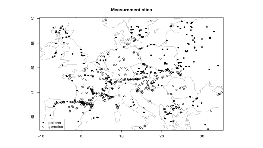
Climate variables are continuous all over Europe but beech forests have specific locations. In order to make our data to spatially coincide, temperature and precipitation curves are firstly estimated on a regular grid of time from 15 Kyears to present on sites where are collected the genetic measures. 15 Kyears corresponds to the beginning of migration of plants onto areas made free by the retreating ice sheets.

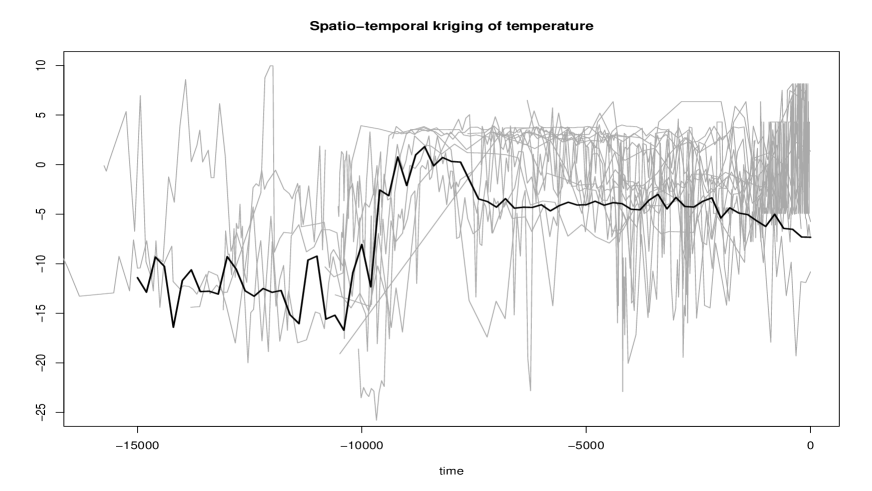
The interpolation is done by a spatio-temporal kriging assuming the covariance function is exponential and separable. Figure 2 shows for a particular site the estimated temperature curve together with some neighboring curves issued from collected pollen.

Figure 2: Resulting temperature curve (thick black curve) from spatio-temporal kriging of 20 neighboring temperatures curves from recorded pollen.

We aim to predict genetic diversity with precipitation and temperature curves. This corresponds to a functional regression model with genetic diversity as dependent variable and temperature and precipitation curves as predictor variable. The cross validation criterion gives better results with an expansion of the predictor variables on a Fourier basis of order 5. Figures 3 and 4 show the coefficient functions $A$, $B$, and kernel $C$.

Figure 3: Coefficient function $A$ of the temperature and coefficient function $B$ of the precipitation

Figure 4: Kernel $C$ of the interaction temperature-precipitation

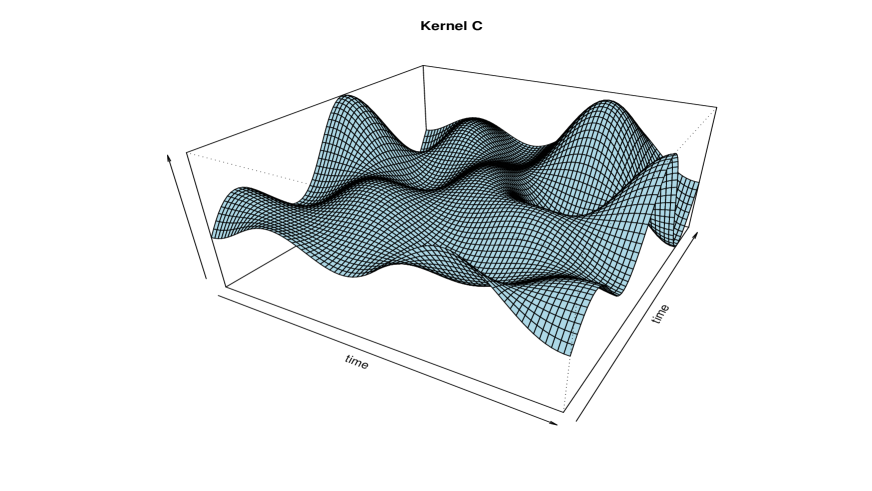
The shape of the coefficient function $A$ shows that the term $\langle A,\theta\rangle$ will be higher when the gap between periods before 7.5 Kyears and after 7.5 Kyears is higher (temperatures before 7.5 Kyears are mostly negative), meanwhile the shape of the coefficient function $B$ shows that the term $\langle B,\pi\rangle$ will be higher when the precipitation before 7.5 Kyears is higher (precipitation is positive). The surface of kernel $C$ is obviously not the product of two curves in the two coordinates, showing an effect of interaction.

In Figure 5 the residual variogram graph exhibits some spatial dependence. An exponential variogram is fitted, and the resulting covariance matrix is plugged into the GLS formula to update the coefficients and test the effects of the temperature, precipitation and interaction.

Figure 5: Empirical and fitted variogram on the residuals.

The graphs in Figure 6 show that the model explains a part of the diversity variability. However it is far from explaining all the variability as the $R^{2}$ is equal to 0.31.

Figure 6: Observed-Predicted response and Predicted-Residuals graphs.

Table 1 gives the analysis of variance of the four nested models:

Model 1:

$\mathbb{E}(Y)=\mu+\langle A;\theta\rangle+\langle B;\pi\rangle+\langle C\theta;\pi\rangle$

Model 2:

$\mathbb{E}(Y)=\mu+\langle A;\theta\rangle+\langle B;\pi\rangle$

Model 3:

$\mathbb{E}(Y)=\mu+\langle A;\theta\rangle$

Model 4:

$\mathbb{E}(Y)=\mu+\langle B;\pi\rangle$

Table 1: Analysis of variance models of nested models

The $p$-values (2.2e-16) of the tests H₀: model 3 (model 4) against H₁: model 2 and (1.430e-07) of the test H₀: model 2 against H₁: model 1 show that the interaction and the two variables have a strong effect.

Figure 7: Pattern of temperature curves according to the range of the predicted response.

Figure 8: Pattern of precipitation curves according to the range of the predicted response.

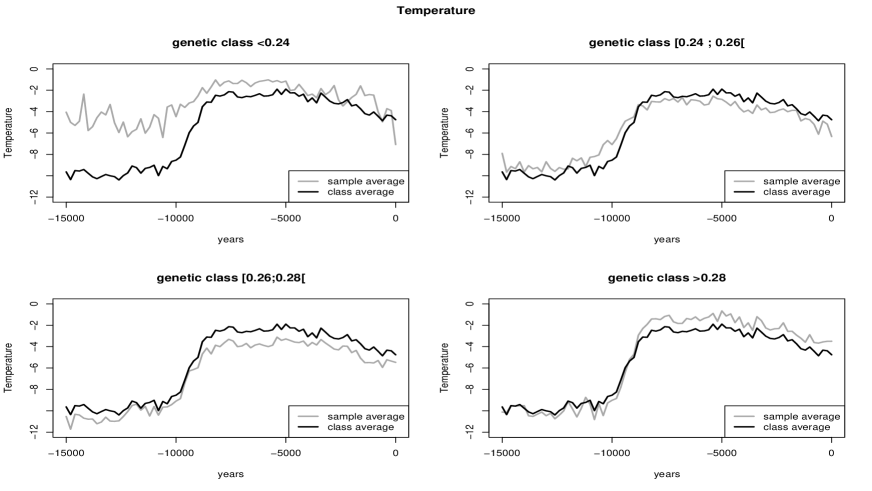
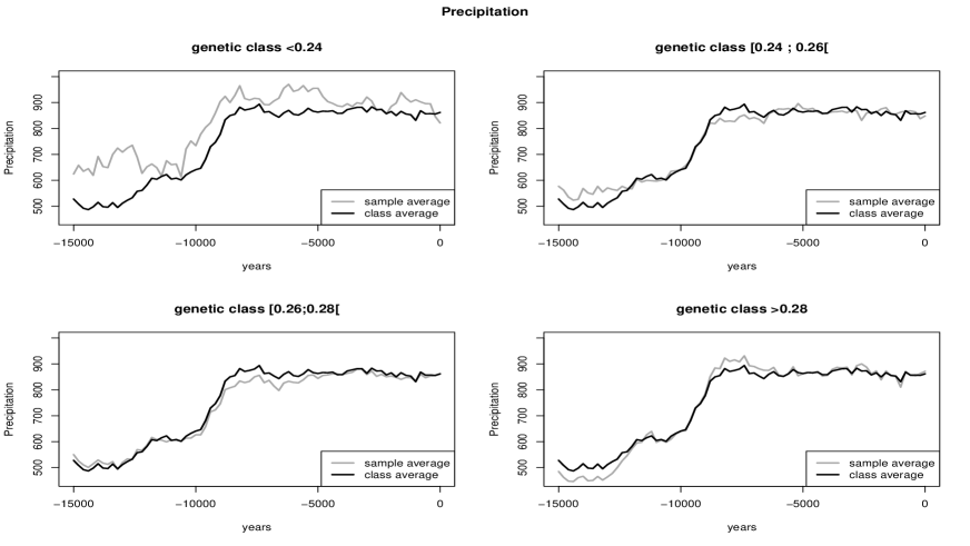
To give a better understanding of the regression model we divide the predicted response range into 4 classes: less than 0.24, ]0.24;0.26], ]0.26;0.28] and greater than 0.28. Figures 7 and 8 show the shapes of temperature and precipitation curves for each class. When low ($<$ 0.24) diversity is predicted, temperature curves are globally higher than the averaged temperature curves on all the sample. As the predicted diversity becomes higher the gap between the two periods before 7.5 Kyears and after 7.5 Kyears gets more pronounced. This effect is less evident for precipitation, low diversity is predicted when the precipitation is higher on the first period than the averaged precipitation curves on all the sample. When the predicted diversity is higher than 0.24 there seems to be no effect of precipitation on its the level.

When the change of climate during the Holocene (12 Kyears to present) is significant the diversity is higher. This mostly concerns northern and western Europe. This is coherent with previous studies cheddadi . After 12 Kyears and throughout the Holocene the climate was no longer uniform all over Europe. The largest mismatch between NW and SE Europe occurred around 9 Kyears and 5 Kyears. By 5 Kyears, all deciduous tree taxa (such as beech) were outside their glacial refugia.

5 Conclusion

The classical linear functional model has been extended in a straightforward manner to the case of two functional predictors with an interaction term, and with spatially correlated residuals. Such a model applied to complex paleoecological and biodiversity data emphasizes an interesting relationship between climate change and genetic diversity: diversity is higher when the change in climate (mostly temperature) during the Holocene (12 Kyears to present) was sizeable and lower when temperature and precipitation are both globally higher over the whole period. This model may be improved in several ways. The spatial effect may be handled in other ways, by means of a mixed structure or with other kinds of correlation matrix structure. In this first attempt we have neglected the random structure and the correlation of the predictors. Taking into account these two characteristics should give a better way to understand the real effect of climate on biodiversity.

References

- [1] H. Cardot, F. Ferraty, P. Sarda, Functional linear model, Statist. Probab. Lett. 45 (1999) 11-22.
- [2] R. Cheddadi, A. Bar-Hen, Spatial gradient of temperature and potential vegetation feedback across Europe during the late Quaternary, Climate Dynamics (in press).
- [3] B. Comps, D. Gömöry, J. Letouzey, B. Thiébaut, R.J. Petit, Diverging trends between heterozygosity and allelic richness during postglacial colonization in the European beech, Genetics 157(2001) 389-397.
- [4] N. Cressie, Statistics for spatial data, Revised Edition, Wiley, New-York, 1993
- [5] D. Dahl-Jensen, K. Mosegaard, N. Gundestrup, G.D. Clow, S.J. Johnsen, A.W. Hansen, N. Balling, Past Temperatures Directly from the Greenland Ice Sheet, Science 282 (1998) 268-271.
- [6] J. Fan, J.T. Zhang, Two-step estimation of functional linear models with application to longitudinal data. J. R. Stat. Soc. Ser. B Stat. Methodol. 62 (2000) 303-322.
- [7] J.J. Faraway, Regression analysis for a functional response, Technometrics 39 (1997) 254-261.
- [8] J. Guiot, Methodology of the last climatic cycle reconstruction in France from pollen data, Palaeogeography Palaeoclimatology Palaeo-ecology 80 (1990) 49-69.
- [9] X. Guyon, Statistique et économétrie, Ellipses Marketing, Paris, 2001
- [10] H.G. Müller, U. Stadtmüller, Generalized functional linear models, Ann. Stat. 33 (2005) 774-806
- [11] J.O. Ramsay, B.W. Silverman, Functional Data Analysis, Springer, New-York, 1997
- [12] J. Seierstad, A. Nesje, S.O. Dahl, J.R. Simonsen, Holocene glacier fluctuations of Grovabreen and Holocene snow-avalanche activity reconstructed from lake sediments in Groningstolsvatnet, western Norway, The Holocene 12:2 (2002) 211-222.