Adiabatic preparation without Quantum Phase Transitions

Abstract

Many physically interesting models show a quantum phase transition when a single parameter is varied through a critical point, where the ground state and the first excited state become degenerate. When this parameter appears as a coupling constant, these models can be understood as straight-line interpolations between different Hamiltonians $H_{\rm I}$ and $H_{\rm F}$. For finite-size realizations however, there will usually be a finite energy gap between ground and first excited state. By slowly changing the coupling constant through the point with the minimum energy gap one thereby has an adiabatic algorithm that prepares the ground state of $H_{\rm F}$ from the ground state of $H_{\rm I}$. The adiabatic theorem implies that in order to obtain a good preparation fidelity the runtime $\tau$ should scale with the inverse energy gap and thereby also with the system size. In addition, for open quantum systems not only non-adiabatic but also thermal excitations are likely to occur. It is shown that – using only local Hamiltonians – for the 1d quantum Ising model and the cluster model in a transverse field the conventional straight line path can be replaced by a series of straight-line interpolations, along which the fundamental energy gap is always greater than a constant independent on the system size. The results are of interest for adiabatic quantum computation since strong similarities between adiabatic quantum algorithms and quantum phase transitions exist.

I Introduction

The promises of quantum computers in solving certain difficult problems such as number factoring shor1997 and database search grover1997a have initiated a lot of research nielsen2000 . As no quantum system can be isolated perfectly from the environment breuer2002 , the influence of decoherence is of great interest. In the conventional scheme of quantum computation, such errors have to be taken into account using expensive error correction schemes or by finding extremely fast quantum gates nielsen2000 . This has drawn attention towards alternative computation schemes such as measurement-based raussendorf2001a ; raussendorf2003a , holonomic pachos2001a or adiabatic farhi2001 quantum computation that either circumvent error-prone parts of the computation process or even provide some intrinsic robustness against imperfect implementation or decoherence.

The basic idea of adiabatic quantum computation (AQC) is to encode the solution to a difficult problem into the ground state of a problem Hamiltonian. A suitable quantum system is prepared in the easily accessible ground state of a different initial Hamiltonian, which is then slowly deformed into the problem Hamiltonian. For slow evolutions the system will remain close to the instantaneous ground state and will therefore finally encode the solution with high fidelity. The adiabatic theorem relates the maximum evolution speed with the spectral properties of the time-dependent Hamiltonian sarandy2004 . Adiabatic quantum computation is polynomially equivalent to the conventional scheme of quantum computation aharonov2007 and it is also believed to be somewhat robust to decoherent interactions at low reservoir temperatures childs2001 : Intuitively, the ground state cannot decay and excitations can only occur for high temperatures. This is also backed by more formal calculations: For a time-independent system Hamiltonian and a thermalized reservoir with inverse temperature $\beta$, the thermalized system density matrix with exactly the same inverse temperature can (in Born-Markov and secular approximation) be shown to be a stationary state of the master equation for the reduced system density matrix breuer2002 . If for system Hamiltonians with a slow time dependence these approximations are also valid childs2001 ; schaller2008a , this would imply robustness of the adiabatic scheme as long as the reservoir temperature is smaller than the fundamental energy gap of the system.

Adiabatic quantum algorithms bear strong similarities to the dynamics through a quantum phase transition latorre2004a ; orus2004a ; sachdev2000 . They connect very different (macroscopically distinguishable) ground states and typically, the fundamental energy gap is well controlled in the beginning and the end of the adiabatic algorithm. Somewhere in between however, the fundamental gap may become very small and for nontrivial problems it will scale inversely with the system size znidaric2005 ; znidaric2006a . Around the minimum energy gap the ground state changes drastically zanardi2006a and in the continuum limit $n\to\infty$, this would correspond to a quantum phase transition where an adiabatic evolution is impossible. However, as one will for AQC always be interested in a finite-size system, the degeneracy between ground state and first excited state is usually replaced by an avoided crossing. Here, the scaling of the energy gap with the system size is of great interest, as it will in practice mean a huge difference whether the gap scales inverse exponentially in $n$ or merely polynomially.

In this paper, two simple models will be studied that conventionally connect two Hamiltonians through a straight-line interpolation, along which in the continuum limit a quantum phase transition is encountered. It will be shown that with using a nonlinear path between the two Hamiltonians, the phase transition can be avoided.

II 1d transverse Ising model

The one-dimensional quantum Ising model in a transverse field sachdev2000 can be envisaged as a straight-line interpolation

$$H(s)=(1-s)H_{\rm I}+sH_{\rm F}$$ (1)

between the initial Hamiltonian $H_{\rm I}$ (at $s=0$) and the final Hamiltonian (at $s=1$)

$$H_{\rm I}=-\sum_{i=1}^{n}\sigma^{x}_{i}\,,\qquad H_{\rm F}=-\sum_{i=1}^{n}\sigma^{z}_{i}\sigma^{z}_{i+1}\,,$$ (2)

where $\sigma^{x/z}_{i}$ denote the Pauli spin matrices acting on the $i^{\rm th}$ qubit and periodic boundary conditions $\sigma^{z}_{n+1}=\sigma^{z}_{1}$ are assumed, which is however not essential for the scaling of the fundamental energy gap.Both Hamiltonians in (2) obey a 180 degree rotational symmetry around all $\sigma^{x}_{i}$-axes (bit-flip), which transforms $\sigma^{z}_{i}$ to $-\sigma^{z}_{i}$.

The ground state of the final Hamiltonian is two-fold degenerate, with $\left|\Psi_{0}^{(1)}\right>=\left|0\ldots 0\right>$ and $\left|\Psi_{0}^{(2)}\right>=\left|1\ldots 1\right>$, where $\sigma^{z}\left|0\right>=+\left|0\right>$ and $\sigma^{z}\left|1\right>=-\left|1\right>$. As the eigenvalues of $H_{\rm F}$ are proportional to the number of kinks in the basis states $\sigma^{z}_{i}\left|z_{1}\dots z_{n}\right>=(-1)^{z_{i}}\left|z_{1}\dots z_{n}\right>$, the two ground states are well separated from the excited states.

The unique ground state of the initial Hamiltonian in (2) is given by

$$\left|{\cal S}\right>=\frac{1}{\sqrt{2^{n}}}\sum_{z=0}^{2^{n}-1}\left|z\right>=\left|\to\right>\otimes\ldots\otimes\left|\to\right>\,,$$ (3)

where $\sigma^{x}\left|\to\right>=+\left|\to\right>$. The excited states (with at least one spin flipped) are again well separated from the ground state.

Due to $\left[H_{\rm F},\bigotimes\limits_{\ell=1}^{n}\sigma^{x}_{\ell}\right]=0$, the bit-flip-parity is a conserved quantity during the interpolation (1), and since (3) is even under bit flip, the final system state will for adiabatic evolution dziarmaga2005a ; cincio2007a ; mostame2007a choose at $s=1$ the even subspace (symmetry breaking) with the huge Schrödinger cat ground state $\left|\Psi_{0}^{\rm even}\right>=1/\sqrt{2}\left[\left|0\ldots 0\right>+\left|1\ldots 1\right>\right]$, if the system is initialized in (3) at $s=0$.

Finally, note that the overlap between initial and final ground state is exponentially small in the system size $n$.

II.1 Straight-Line Interpolation

At any point during the interpolation $s\in[0,1]$, the Hamiltonian $H(s)$ can be diagonalized: The successive application of Jordan-Wigner, Fourier and Bogoliubov transformations jordan1928a ; sachdev2000 map the spin-1/2-Hamiltonian to a fermionic one, which (in the subspace of even bit-flip parity corresponding to even numbers of quasi-particles only) reads

$$H(s)=\sum_{k}\epsilon_{k}\left(\gamma_{k}^{\dagger}\gamma_{k}-\frac{1}{2}\right)\,,$$ (4)

with the fermionic operators $\gamma_{k}$ and single quasi-particle energies

$$\epsilon_{k}=\sqrt{1-4\cos^{2}(ka/2)s(1-s)}\,,$$ (5)

see figure 1 left panel. The wavenumber $ka$ covers the range $ka=\frac{\pi}{n}\left(1+2\mathbb{Z}\right)\qquad:\qquad{\left|ka\right|}<\pi$.

From equation (5) one obtains a minimum gap of $g_{\rm min}=2\sin\left(\frac{\pi}{2n}\right)={\cal O}\{1/n\}$ and indeed one also observes for constant speed interpolation $s=t/\tau$ a quadratic scaling of the adiabatic runtime $\tau_{\rm ad}={\cal O}\{n^{2}\}$ dziarmaga2005a with the number of qubits $n$. At the critical point $s_{\rm crit}=1/2$, the Ising model undergoes a second order quantum phase transition sachdev2000 , which manifests itself in a divergence of the second derivative of the ground state energy.

II.2 Nonlinear Interpolation Path

The linear interpolation scheme in equation (1) is rather simple but not necessary for the adiabatic theorem to hold farhi0208135 ; siu2007a . The nonlinear interpolation we will consider here will connect the Hamiltonians of (2) by a series of straight-line interpolations along the Hamiltonians

$$H_{0} = -\sum_{i=1}^{n}\sigma^{x}_{i}=H_{\rm I}\,,$$

$$H_{1} = -\sigma^{z}_{1}\sigma^{z}_{2}-\sum_{i=3}^{n}\sigma^{x}_{i}\,,$$

$$\vdots$$

$$H_{k} = -\sum_{i=1}^{k}\sigma^{z}_{i}\sigma^{z}_{i+1}-\sum_{i=k+2}^{n}\sigma^{x}_{i}\,,$$

$$\vdots$$

$$H_{n-1} = -\sum_{i=1}^{n-1}\sigma^{z}_{i}\sigma^{z}_{i+1}\,,$$

$$H_{n} = -\sum_{i=1}^{n}\sigma^{z}_{i}\sigma^{z}_{i+1}=H_{\rm F}\,,$$ (6)

such that formally the time-dependent Hamiltonian is given by

$$H(t) = \sum_{k=0}^{n-1}\Theta\left[s_{k}(t)\right]\Theta\left[1-s_{k}(t)\right]\times$$ (7)

$$\times \left\{\left[1-s_{k}(t)\right]H_{k}+s_{k}(t)H_{k+1}\right\}\,,$$

where $\Theta(x)$ denotes the Heavyside step function and $s_{k}(t)=\frac{t-k\Delta t}{\Delta t}$ encodes a constant speed interpolation with $n\Delta t=\tau$ such that $s_{k}[(k+1)\Delta t]=1=1-s_{k+1}[(k+1)\Delta t]$ and $H(\tau)=H_{\rm F}$.

Given a spin chain with (constant) $\sigma^{z}_{i}\sigma^{z}_{i+1}$-interactions, one has to apply a correspondingly stronger external field to achieve an effective decoupling of the spins. Physically the above nonlinear scheme could be approximated by a strong transverse magnetic field that within the distance between two spins rises linearly from zero to maximum and then travels at constant speed along the spin chain. Conversely, one might imagine to slowly pull the spin chain out of a region with a strong stationary transverse field. Recent proposals for quantum simulators of the Ising model in a transverse field porras2004a ; mostame0803 however, even provide a more direct control of the local spin-spin interactions, such that all regions of the phase diagram can in principle be reached.

Note that the interpolation path (II.2) does not destroy the bitflip symmetry, since $\left[H_{k},\bigotimes\limits_{\ell=1}^{n}\sigma^{x}_{\ell}\right]=0$. It is easy to see that the ground state of a Hamiltonian $H_{k}$ in (II.2) (within the subspace of even bit-flip parity) is for $1\leq k\leq n-1$ given by

$$\left|\Psi_{k}^{\rm 0,even}\right>=\frac{1}{\sqrt{2}}\left[\mbox{\boldmath$1$}+\sigma^{x}_{1}\ldots\sigma^{x}_{k+1}\right]{\cal H}_{k+2}\ldots{\cal H}_{n}\left|0\ldots 0\right>\,,$$ (8)

where ${\cal H}_{k}=\frac{1}{\sqrt{2}}\left(\sigma^{x}_{k}+\sigma^{z}_{k}\right)$ denotes the Hadamard gate on qubit $k$, such that the overlap between two successive ground states yields $\left<\Psi_{k}^{\rm 0,even}|\Psi_{k+1}^{\rm 0,even}\right>=1/\sqrt{2}$ for $0\leq k\leq n-2$. In the last interpolation step, the ground state is even invariant $\left<\Psi_{n-1}^{\rm 0,even}|\Psi_{n}^{\rm 0,even}\right>=1$. Hence, in every single step only slight transformations of the ground state are performed and intuitively, one may expect that adiabatic preparation along this modified path should be more efficient than in the conventional scheme.

For the first interpolation step $H_{0}(s)\equiv(1-s)H_{0}+sH_{1}$ in (II.2), the first two qubits evolve independently from the rest of the system and it is straightforward to obtain the eigenvalues from the nontrivial contribution of their four-dimensional subspace

$$\lambda_{0}^{\kappa} = -\sqrt{5s^{2}-8s+4}-(n-2)+2\kappa\,,$$

$$\lambda_{1}^{\kappa} = -s-(n-2)+2\kappa\,,$$

$$\lambda_{2}^{\kappa} = +s-(n-2)+2\kappa\,,$$

$$\lambda_{3}^{\kappa} = +\sqrt{5s^{2}-8s+4}-(n-2)+2\kappa\,,$$ (9)

where $\kappa\in\{0,1,\ldots,(n-2)\}$ counts the excitations resulting from qubits $3\ldots n$, see figure 1 right panel.

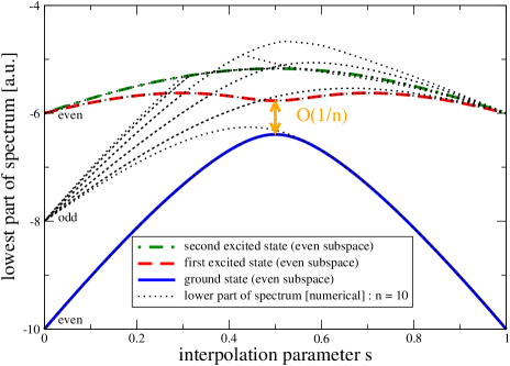
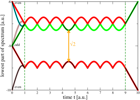
Figure 1: [Color Online] Left: Lowest eigenvalues for the 1d quantum Ising model in a transverse field (2) and linear interpolation (1) for $n=10$. Thick lines show the analytical result for the eigenvalues of the even subspace (5), whereas the thin dotted lines give the numerical result arpack1998 for all lowest eigenvalues. Right: Comparison of numerical calculation (dense symbols visible as thick lines) with the analytical prediction for $\kappa=0$ (solid black lines, only shown in intervals $[0,1]$, $[4,5]$, $[9,10]$) for stepwise interpolation (II.2) with $n=10$ and $\tau=10$. The different interpolation regimes are separated by dashed vertical lines. Throughout the interpolation scheme the minimum gap in the even subspace is always larger than $\sqrt{2}$. The ARPACK package arpack1998 only determines one part (e.g., the lower) of the spectrum, which is why not all numerical eigenvalues are shown.

By continuity we identify $\lambda_{0}^{0}$ and $\lambda_{3}^{0}$ as belonging to the even subspace and thus one obtains in the first interpolation step for the minimum gap $g_{\rm min}^{\rm even}=\min\left[\lambda_{3}^{0}-\lambda_{0}^{0}\right]=4/\sqrt{5}$ at $s_{\rm min}=4/5$.

For the intermediate steps we have

$$H_{k}(s) \equiv (1-s)H_{k}+sH_{k+1}$$ (10)

$$= -\sum_{i=1}^{k}\sigma^{z}_{i}\sigma^{z}_{i+1}-\sum_{i=k+3}^{n}\sigma^{x}_{i}$$

$$-(1-s)\sigma^{x}_{k+2}-s\sigma^{z}_{k+1}\sigma^{z}_{k+2}$$

in (II.2) for $1\leq k\leq n-2$. In order to obtain the spectrum conveniently, we will map the Hamiltonian using a suitable unitary transformation to another one which can be diagonalized easily. For the Ising model we consider the controlled NOT-gate

$$S_{ij}^{\rm CNOT}=\frac{1}{2}\left(\mbox{\boldmath$1$}_{i}+\sigma^{z}_{i}\right)\otimes\mbox{\boldmath$1$}_{j}+\frac{1}{2}\left(\mbox{\boldmath$1$}_{i}-\sigma^{z}_{i}\right)\otimes\sigma^{x}_{j}\,,$$ (11)

which is a Hermitian controlled-unitary operation nielsen2000 , where $i$ is the control and $j$ the target qubit. It is straightforward to show that

$$S_{ij}^{\rm CNOT}\left[\sigma^{z}_{i}\otimes\mbox{\boldmath$1$}_{j}\right]S_{ij}^{\rm CNOT} = \sigma^{z}_{i}\otimes\mbox{\boldmath$1$}_{j}\,,$$

$$S_{ij}^{\rm CNOT}\left[\sigma^{z}_{i}\otimes\sigma^{z}_{j}\right]S_{ij}^{\rm CNOT} = \mbox{\boldmath$1$}_{i}\otimes\sigma^{z}_{j}\,,$$

$$S_{ij}^{\rm CNOT}\left[\mbox{\boldmath$1$}_{i}\otimes\sigma^{x}_{j}\right]S_{ij}^{\rm CNOT} = \mbox{\boldmath$1$}_{i}\otimes\sigma^{x}_{j}\,.$$ (12)

Using the CNOT transformation at the transition region, the Hamiltonian (10) is mapped to

$$S_{k+1,k+2}^{\rm CNOT}H_{k}(s)S_{k+1,k+2}^{\rm CNOT} = -\sum_{i=1}^{k}\sigma^{z}_{i}\sigma^{z}_{i+1}-\sum_{i=k+3}^{n}\sigma^{x}_{i}$$ (13)

$$-(1-s)\sigma^{x}_{k+2}-s\sigma^{z}_{k+2}\,,$$

where it is visible that the qubit sets $\{1,\ldots,(k+1)\}$, $\{(k+2)\}$, and $\{(k+3),\ldots,n\}$ are mutually decoupled. Evidently, one obtains for qubits $1\ldots(k+1)$ just the eigenvalues of the Ising model with open boundary conditions (i.e., with minimum energy $-k$ for a two-fold degenerate ground state and fundamental energy gap 2) and for qubits $(k+3),\ldots,n$ a minimum energy of $-(n-k-2)$ for the unique ground state and a fundamental energy gap of 2. The nontrivial part of the spectrum arises from the subspace of qubit $(k+2)$, where one obtains for the eigenvalues

$$\lambda_{\pm}^{\kappa}=\pm\sqrt{1-2s(1-s)}-(n-2)+2\kappa\,,$$ (14)

where $\kappa\in\{0,1,\ldots,(n-2)\}$, see figure 1 right panel. Therefore, the fundamental energy gap equates to $g_{\rm min}^{\rm even}=\sqrt{2}$, which is independent on the system size.

The last step is trivial: As $\left[H_{n-1},H_{n}\right]=0$, both Hamiltonians can be diagonalized simultaneously and the spectra of $H_{n-1}$ and $H_{n}$ are therefore just connected by straight lines as is also visible in figure 1 right panel.

Therefore, we obtain with the new interpolation path a lower bound on the minimum fundamental energy gap

$$g_{\rm min}^{\rm even}\geq\sqrt{2}$$ (15)

in the even subspace. Note that as a sanity check, in figure 1 right panel a perfect agreement is found between analytically and numerically calculated eigenvalues arpack1998 is found.

In the absence of a reservoir one would have an adiabatic scheme to efficiently prepare large Schrödinger cat states: If the quantum system is initialized in its initial ground state (3) (by applying a strong magnetic field) and then slowly evolved through the series of interpolations towards $H_{\rm F}$, the adiabatic theorem will guarantee that the system will remain close to its instantaneous ground state. Evidently, the last step in (II.2) can also be omitted without changing the ground state, just the energies will differ. This does not mean that one can adiabatically deform $H_{\rm I}$ in $H_{\rm F}$ in (2) in constant time, as the number of steps in (7) scales linearly with the system size $n$. In order to obtain a fixed final fidelity of the desired state $\left|\Psi_{\rm final}\right>=1/\sqrt{2}\left[\left|0\ldots 0\right>+\left|1\ldots 1\right>\right]$, the adiabatic runtime $\tau_{\rm ad}$ will scale nearly linearly with the system size $\tau_{\rm ad}\propto n\log n$ for the new scheme (II.2) instead of quadratically dziarmaga2005a for the straight-line interpolation scheme (1). The logarithmic corrections are expected from the increasing number of degeneracies in the first excited states schaller2006a . However, this favorable scaling could also have been achieved by using the conventional scheme (1) with straight-line but adaptive-speed interpolation schaller2006a ; jansen2007a . Therefore, the advantage of the nonlinear scheme is rather given by the fact that constant-speed interpolation suffices and – more importantly – for couplings to a reservoir that do not destroy the bitflip symmetry the new scheme provides some resistance to thermal excitations as long as $k_{\rm B}T_{\rm res}<{\cal O}\{1\}$.

For realistic systems however it is to be expected that the conservation of bit-flip parity will be destroyed by the existence of a reservoir, such that amplitude from the even subspace may leak into the subspace of odd bitflip parity mostame2007a ; fubini2007a (such effects may also limit the robustness of other models against decoherence, see e.g. balachandran2008a ). The net effect would be the decay of the desired Schrödinger cat state. In principle, this could be avoided with an additional (time-independent) Hamiltonian of the form

$$\Delta H_{\rm F} = \frac{\alpha}{2}\left[\mbox{\boldmath$1$}-\bigotimes\limits_{\ell=1}^{n}\sigma^{x}_{\ell}\right]\,,$$

to safely separate the even and odd subspaces. Unfortunately, it involves $n$-qubit interactions and is thus presumably difficult to implement. In the following, we will therefore consider a model with a local Hamiltonian that has a unique ground state.

III Preparation of the Cluster State

The cluster state on a lattice ${\cal L}$ can be encoded in the ground state of the Hamiltonian

$$H=-\sum_{\mu\in{\cal L}}\sigma^{x}_{\mu}\bigotimes_{\nu\stackrel{{\scriptstyle\cal L}}{{\sim}}\mu}\sigma^{z}_{\nu}\,,$$ (17)

where $\nu\stackrel{{\scriptstyle\cal L}}{{\sim}}\mu$ denotes all sites $\nu$ that are connected to the site $\mu$ in the lattice $\cal L$ by a link. In order to see that the cluster state is the ground state of (17), we use the controlled Z-gate

$$S_{ij}^{\rm CZ}=\frac{1}{2}\left(\mbox{\boldmath$1$}_{i}+\sigma^{z}_{i}\right)\otimes\mbox{\boldmath$1$}_{j}+\frac{1}{2}\left(\mbox{\boldmath$1$}_{i}-\sigma^{z}_{i}\right)\otimes\sigma^{z}_{j}=S_{ji}^{\rm CZ}\,,$$ (18)

which acts as

$$S_{ij}^{\rm CZ}\left|z_{i}\right>\otimes\left|z_{j}\right>=(-1)^{z_{i}z_{j}}\left|z_{i}\right>\otimes\left|z_{j}\right>$$ (19)

in the computational basis. Obviously, it is Hermitian and $\left[S_{ij}^{\rm CZ},S_{kl}^{\rm CZ}\right]=0$, such that we can unambiguously define the global unitary operation

$$S_{\cal L}=\prod_{\nu\stackrel{{\scriptstyle\cal L}}{{\sim}}\mu}S_{\mu\nu}^{\rm CZ}=S_{\cal L}^{\dagger}\,.$$ (20)

With using the relations (see also doherty08024314 )

$$S_{ij}^{\rm CZ}\left[\sigma^{z}_{i}\otimes\sigma^{x}_{j}\right]S_{ij}^{\rm CZ} = \mbox{\boldmath$1$}_{i}\otimes\sigma^{x}_{j}\,,$$

$$S_{ij}^{\rm CZ}\left[\sigma^{z}_{i}\otimes\mbox{\boldmath$1$}_{j}\right]S_{ij}^{\rm CZ} = \sigma^{z}_{i}\otimes\mbox{\boldmath$1$}_{j}\,,$$

$$S_{ij}^{\rm CZ}\left[\mbox{\boldmath$1$}_{i}\otimes\sigma^{z}_{j}\right]S_{ij}^{\rm CZ} = \mbox{\boldmath$1$}_{i}\otimes\sigma^{z}_{j}$$ (21)

it is easy to see that the unitary transformation (20) maps the Hamiltonian (17) into decoupled spins

$$S_{\cal L}HS_{\cal L}^{\dagger}=-\sum_{\mu\in{\cal L}}\sigma^{x}_{\mu}\,.$$ (22)

This implies that the ground state of (17) is unique and separated by a safe energy gap of $\Delta E=2$ from the first excited states. From the ground state of (22) it can be obtained via

$$\left|\Psi_{\rm cl}\right> = S_{\cal L}\left|\to\right>\otimes\ldots\otimes\left|\to\right>$$ (23)

$$= \frac{1}{\sqrt{2^{n}}}\sum_{z=0}^{2^{n}-1}(-1)^{\sum\limits_{\mu\nu}L_{\mu\nu}z_{\mu}z_{\nu}}\left|z_{1}\ldots z_{n}\right>\,,$$

where $L_{\mu\nu}=1$ if $\mu\stackrel{{\scriptstyle\cal L}}{{\sim}}\nu$ and $L_{\mu\nu}=0$ otherwise, and $n={\left|\cal L\right|}$ denotes the number of lattice sites. Above equation already gives the recipe of preparing the cluster state using only the two-qubit unitary operations (18). However, considering the destructive influence of an environment it would be desirable to encode the cluster state in the ground state of a Hamiltonian, which could then be reached by adiabatic transformation, see below.

III.1 The 1d cluster state

In analogy to the Ising model in a transverse field (2), one could prepare the cluster state on a 1d spin chain adiabatically by a straight line interpolation (1) between

$$H_{\rm I} = -\sum_{i=1}^{n}\sigma^{x}_{i}\qquad\mbox{and}$$

$$H_{\rm F} = -\sigma^{x}_{1}\sigma^{z}_{2}-\left[\sum_{i=2}^{n-1}\sigma^{z}_{i-1}\sigma^{x}_{i}\sigma^{z}_{i+1}\right]-\sigma^{z}_{n-1}\sigma^{x}_{n}\,,$$ (24)

what is referred to as ’transverse field cluster model’ in doherty08024314 . It has been shown that the above model exhibits a quantum phase transition at $s_{\rm crit}=1/2$ pachos2004a , which can be understood as (III.1) can be mapped via a duality transformation to two Ising models in a transverse field doherty08024314 . Accordingly, this kind of preparation would be vulnerable to nonadiabatic and thermal excitations in the large $n$ limit, as the minimum energy gap will scale as ${\cal O}\{1/n\}$, see also figure 3 left panel.

Therefore, we will consider the stepwise interpolation scheme (7) along

$$H_{0} = -\sum_{i=1}^{n}\sigma^{x}_{i}=H_{\rm I}\,,$$

$$H_{1} = -\sigma^{x}_{1}\sigma^{z}_{2}-\sigma^{z}_{1}\sigma^{x}_{2}-\sum_{i=3}^{n}\sigma^{x}_{i}\,,$$

$$H_{2} = -\sigma^{x}_{1}\sigma^{z}_{2}-\sigma^{z}_{1}\sigma^{x}_{2}\sigma^{z}_{3}-\sigma^{z}_{2}\sigma^{x}_{3}-\sum_{i=4}^{n}\sigma^{x}_{i}\,,$$

$$\vdots$$

$$H_{k} = -\sigma^{x}_{1}\sigma^{z}_{2}-\sum_{i=2}^{k}\sigma^{z}_{i-1}\sigma^{x}_{i}\sigma^{z}_{i+1}-\sigma^{z}_{k}\sigma^{x}_{k+1}-\sum_{i=k+2}^{n}\sigma^{x}_{i}$$ (25)

$$= -\sum_{\mu\in{\cal L}_{k}}\sigma^{x}_{\mu}\bigotimes_{\nu\stackrel{{\scriptstyle{\cal L}_{k}}}{{\sim}}\mu}\sigma^{z}_{\nu}\,.$$

The physical implementation of such a model would of course be more demanding: Given that the necessary three-body interactions can be simulated by logical qubits (possibly built of several physical ones along the lines of bartlett2006a ), the region of a non-vanishing transverse field gradient should here also be confined within the distance between two logical qubits. In order to simplify the notation, we have written the intermediate Hamiltonian of (III.1) as in (17) and just modify the number of existent links in the lattices ${\cal L}_{k}$, see figure 2.

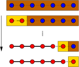
Figure 2: [Color Online] Stepwise buildup of the cluster state on a 1d spin chain with $n=7$ spins within 6 steps using a runtime of $\tau={\cal O}\{n\}$. In lattice ${\cal L}_{1}$, all spins are unconnected (dark-blue) and in lattice ${\cal L}_{2}$ only two spins are connected (grey-red) by solid lines. Thin dotted lines show the intended order of inclusion in the connected sublattice. Dark shaded regions (brown) show the presence of a strong transverse field, whereas in the light-shaded regions (yellow) the field is gradually decreased from maximum to zero.

Then, we obtain for an intermediate interpolation step

$$H_{k}(s) \equiv (1-s)H_{k}+sH_{k+1}$$ (26)

$$= -\sigma^{x}_{1}\sigma^{z}_{2}-\sum_{i=2}^{k}\sigma^{z}_{i-1}\sigma^{x}_{i}\sigma^{z}_{i+1}-\sum_{i=k+3}^{n}\sigma^{x}_{i}$$

$$-(1-s)\sigma^{z}_{k}\sigma^{x}_{k+1}-(1-s)\sigma^{x}_{k+2}$$

$$-s\sigma^{z}_{k}\sigma^{x}_{k+1}\sigma^{z}_{k+2}-s\sigma^{z}_{k+1}\sigma^{x}_{k+2}\,,$$

where it becomes visible that by applying the global unitary only on the existing links in lattice ${\cal L}_{k}$, the model is again decoupled nearly completely

$$S_{{\cal L}_{k}}H_{k}(s)S_{{\cal L}_{k}}^{\dagger} = -\sum_{i=1\;:\;i\notin\{(k+1),(k+2)\}}^{n}\sigma^{x}_{i}$$ (27)

$$-s\left(\sigma^{x}_{k+1}\sigma^{z}_{k+2}+\sigma^{z}_{k+1}\sigma^{x}_{k+2}\right)$$

$$-(1-s)\left(\sigma^{x}_{k+1}+\sigma^{x}_{k+2}\right)\,.$$

In above equation, only qubits $\{(k+1),(k+2)\}$ contribute the nontrivial parts of the spectrum and we obtain for the eigenvalues

$$\lambda_{1}^{\kappa} = -2\sqrt{1-2s(1-s)}-(n-2)+2\kappa\,,$$

$$\lambda_{2}^{\kappa} = \lambda_{3}^{\kappa}=-(n-2)+2\kappa\,,$$

$$\lambda_{4}^{\kappa} = +2\sqrt{1-2s(1-s)}-(n-2)+2\kappa$$ (28)

with $\kappa\in\{0,1,\ldots,(n-2)\}$. Note that the first interpolation step yields the same eigenvalues, as is also visible in the numerical calculation of the spectrum, see figure 3 right panel.

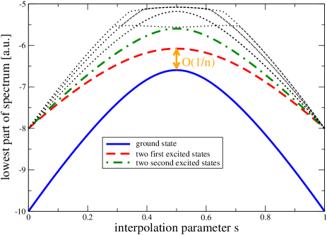
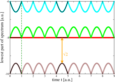
Figure 3: [Color Online] Left:Numerical Calculation of the lowest eigenvalues for the adiabatic cluster model in a transverse field (17) for $n=10$. Thick lines show the lowest five eigenvalues. Right:Numerical Calculation of the lowest eigenvalues for the stepwise cluster model (III.1) for $n=10$ and $\Delta t=1$. Analytical predictions (solid lines) resulting from (III.1) for $\kappa=0$ perfectly match the numerical results.

III.2 The 2d cluster state

In 2d, the cluster state can serve as a universal resource for measurement-based quantum computation raussendorf2001a ; raussendorf2003a . Therefore, we will here also state some known facts about its adiabatic preparation via a straight-line interpolation (1) between the Hamiltonians

$$H_{\rm I}=-\sum_{\mu\in{\cal L}}\sigma^{x}_{\mu}\,,\qquad H_{\rm F}=-\sum_{\mu\in{\cal L}}\sigma^{x}_{\mu}\bigotimes_{\nu\stackrel{{\scriptstyle{\cal L}}}{{\sim}}\mu}\sigma^{z}_{\nu}\,,$$ (29)

where ${\cal L}$ denotes a square lattice, such that five-body interactions are required in order to implement $H_{\rm F}$. For the direct straight-line interpolation one can map the above model with a duality transformation doherty08024314 to one with a known quantum phase transition at $s_{\rm crit}=1/2$ xu2004a .

It is easy to see that one can choose an interpolation scheme where either only one or two links are added at once, see figure 4.

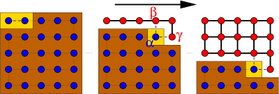
Figure 4: [Color Online] Stepwise buildup of the cluster state on a 2d spin lattice with $n=25$ spins in 24 steps. Thin dotted lines show the intended order of inclusion in the connected sublattice. In each single step, either only one or two links are added. With regard to realization, one could imagine a region with a strong transverse magnetic field (dark-brown shaded region), which is turned off slowly (light-yellow shaded region) along a rectangular zig-zag trajectory as outlined by the thin dotted lines.

Whenever only a single link is inserted, we have the same situation as in the 1d case, therefore we will consider the more interesting case of adding two links at once here. Suppose a node $\alpha$ is unconnected in lattice ${\cal L}_{k}$ (i.e., at $s=0$ with Hamiltonian $H_{k}$) and shall be connected to two other nodes $\beta$ and $\gamma$ in lattice ${\cal L}_{k+1}$ (i.e., at $s=1$ with Hamiltonian $H_{k+1}$). Suppose also that the nodes $\beta$ and $\gamma$ are already connected to other nodes in lattice ${\cal L}_{k}$ as depicted in figure 4. Then, the corresponding Hamiltonian can be written as

$$H_{k}(s) \equiv (1-s)H_{k}+sH_{k+1}$$ (30)

$$= -\sum_{\mu\neq\alpha\beta\gamma}\sigma^{x}_{\mu}\bigotimes_{\nu\stackrel{{\scriptstyle{\cal L}_{k}}}{{\sim}}\mu}\sigma^{z}_{\nu}$$

$$-s\left(\sigma^{x}_{\alpha}\sigma^{z}_{\beta}\sigma^{z}_{\gamma}+\sigma^{z}_{\alpha}\sigma^{x}_{\beta}\bigotimes_{\nu\stackrel{{\scriptstyle{\cal L}_{k}}}{{\sim}}\beta}\sigma^{z}_{\nu}+\sigma^{z}_{\alpha}\sigma^{x}_{\gamma}\bigotimes_{\nu\stackrel{{\scriptstyle{\cal L}_{k}}}{{\sim}}\gamma}\sigma^{z}_{\nu}\right)$$

$$-(1-s)\left(\sigma^{x}_{\alpha}+\sigma^{x}_{\beta}\bigotimes_{\nu\stackrel{{\scriptstyle{\cal L}_{k}}}{{\sim}}\beta}\sigma^{z}_{\nu}+\sigma^{x}_{\gamma}\bigotimes_{\nu\stackrel{{\scriptstyle{\cal L}_{k}}}{{\sim}}\gamma}\sigma^{z}_{\nu}\right).$$

Using the unitary transformation $S_{{\cal L}_{k}}$, we again arrive at a nearly decoupled model (where only three spins are mutually coupled)

$$S_{{\cal L}_{k}}H(s)S_{{\cal L}_{k}}^{\dagger} = -\sum_{\mu\neq\alpha\beta\gamma}\sigma^{x}_{\mu}-(1-s)\left(\sigma^{x}_{\alpha}+\sigma^{x}_{\beta}+\sigma^{x}_{\gamma}\right)$$ (31)

$$-s\left(\sigma^{x}_{\alpha}\sigma^{z}_{\beta}\sigma^{z}_{\gamma}+\sigma^{z}_{\alpha}\sigma^{x}_{\beta}+\sigma^{z}_{\alpha}\sigma^{x}_{\gamma}\right)\,.$$

Evaluating the eigenvalues of the $8\times 8$ matrix generated by qubits $\{\alpha,\beta,\gamma\}$ yields (for simplicity we only give the two lowest eigenvalues)

$$\lambda_{0}^{\kappa} = -\sqrt{5-10s(1-s)+2\sqrt{4(1-2s)^{2}+25s^{2}\left(1-s\right)^{2}}}$$

$$-(n-3)+2\kappa\,,$$

$$\lambda_{1}^{\kappa} = -1-(n-3)+2\kappa\,,$$ (32)

where $\kappa\in\{0,1,\ldots,(n-3)\}$. Therefore, we obtain a fundamental energy gap of $g_{\rm min}=\sqrt{5}-1$ at $s_{\rm min}=1/2$, which is independent on the system size.

Note that we have so far allowed the external field to vary at a single site on the lattice only. If one does not have this constraint many of the steps can be performed in parallel, such that the overall time required to generate the cluster state is further reduced, compare also siu2007a .

IV Adiabatic Quantum Computation

In the previous sections it was shown for specific models that quantum phase transitions encountered along a straight-line path can be avoided if a nonlinear path is chosen. It would be great if this could be extended to adiabatic quantum computation, where for the nontrivial models numerical calculations based on a straight-line interpolation point to an inverse scaling of the fundamental energy gap with the system size znidaric2005 ; znidaric2006a ; latorre2004a ; orus2004a ; schuetzhold2006b . Not only would such a path usually admit a significantly shortened runtime of the adiabatic algorithm but also concerning robustness against thermal excitations a constant lower bound on the fundamental energy gap would be highly desirable. As a first step, we will show that there exist paths consisting of a series of straight-line interpolations, along which the fundamental gap can be calculated analytically. As one paradigmatic example for the problem class NP, we will illustrate this for Exact Cover 3 (EC3), which is a special case of 3-SAT. The EC3-problem can be defined as follows farhi2001 : Given $m$ clauses each involving positions of three bits $C_{i}=(p_{i}^{1},p_{i}^{2},p_{i}^{3})$ with $1\leq i\leq m$ and $1\leq p_{i}^{\alpha}\leq n$ one is looking for the $n$-bit bitstring $\{b_{1}\ldots b_{n}\}$ with $b_{i}\in\{0,1\}$ that fulfills for each clause $b_{p_{i}^{1}}+b_{p_{i}^{2}}+b_{p_{i}^{3}}=1$, where ’$+$’ denotes the integer sum. A problem Hamiltonian encoding the solution to the EC3 problem in its ground state can be given as banuls2006a ; schuetzhold2006b

$$H_{\rm P} = \sum_{i=1}^{m}\left[\mbox{\boldmath$1$}-\hat{z}_{p_{i}^{1}}-\hat{z}_{p_{i}^{2}}-\hat{z}_{p_{i}^{3}}\right]^{2}$$ (33)

where $\hat{z}_{k}=\frac{1}{2}\left(\mbox{\boldmath$1$}-\sigma^{z}_{k}\right)$.

Unfortunately, since the neighborship topology in the irregular lattice defined by $n_{ij}$ in an EC3 problem cannot be represented by next neighbor interactions for a fixed dimensionality and does not even have a regular structure, there is no obvious unique way of defining a nonlinear interpolation scheme, compare also farhi0208135 . Here, it will be proposed that by turning on the clauses one by one in (33) whilst maintaining a unique ground state one should obtain a considerable improvement in the fundamental energy gap for the average EC3 problem. We define a partial problem Hamiltonian via

$$H_{\rm P}^{k}=\left[\mbox{\boldmath$1$}-\hat{z}_{p_{k}^{1}}-\hat{z}_{p_{k}^{2}}-\hat{z}_{p_{k}^{3}}\right]^{2}$$ (34)

The series of Hamiltonians in the nonlinear path can then be written as

$$H_{k}=\mbox{\boldmath$1$}-\left|\Psi_{k}\right>\left<\Psi_{k}\right|$$ (35)

connected by stepwise linear interpolations (7) for $0\leq k\leq m$ and where the unique ground states are the symmetrized superpositions of solutions to a subset of clauses

$$\left|\Psi_{k}\right>=\frac{1}{\sqrt{N_{k}}}\sum_{z\;:\;\left(H_{\rm P}^{1}+\ldots+H_{\rm P}^{k}\right)\left|z\right>=0}\left|z\right>\,,$$ (36)

where we have denoted the ground state degeneracy of $H_{\rm P}^{1}+\ldots+H_{\rm P}^{k}$ by $N_{k}$. This of course does not uniquely define an interpolation scheme, since we may exchange the order of clauses without changing the final solution. For the linear interpolation between two projector Hamiltonians $H_{k}(s)=\mbox{\boldmath$1$}-(1-s)\left|\Psi_{k}\right>\left<\Psi_{k}\right|-s\left|\Psi_{k+1}\right>\left<\Psi_{k+1}\right|$, the simple result for the adiabatic Grover algorithm roland2002 may be easily generalized wei2006a to obtain the eigenvalues $\lambda_{0/1}=\frac{1}{2}\left(1\pm\sqrt{1-4s(1-s)\left(1-{\left|\left<\Psi_{k}|\Psi_{k+1}\right>\right|}^{2}\right)}\right)$ and $\lambda_{2}=\ldots=\lambda_{2^{n}-1}=1$, such that the minimum fundamental energy gap equates to $g_{\rm min}={\left|\left<\Psi_{k}|\Psi_{k+1}\right>\right|}=\sqrt{\frac{N_{k+1}}{N_{k}}}\equiv\sqrt{r_{k}}$ (where $r_{k}\leq 1$ is the reduction factor in the number of solutions at step $k$). For an average EC3 problem with a unique solution, this would be a significant improvement, since typically a modest number of states will violate only a single clause. For extreme problems however, an exponential number of basis states could possibly just violate only a single clause, such that even re-ordering of the clauses would not yield a polynomial scaling of the fundamental energy gap. However, for direct interpolation between $H_{0}$ and $H_{m}$ (where we would reproduce the adiabatic Grover algorithm roland2002 ) we obtain (for a problem with a unique solution such that $N_{m}=1$) the minimum fundamental gap of $g_{\rm min}^{\rm direct}=1/\sqrt{2^{n}}$, which is always significantly smaller than the smallest gap that could be encountered with stepwise interpolation.

A further drawback of the scheme is that the Hamiltonians (35) are generally nonlocal and cannot be efficiently implemented, as can for example be seen from the formal representation of its ground state

$$\left|\Psi_{k}\right>=\sqrt{\frac{N}{N_{k}}}\left[\prod_{\ell=1}^{k}\left(\mbox{\boldmath$1$}-H_{\rm P}^{\ell}\right)\left(\mbox{\boldmath$4$}-H_{\rm P}^{\ell}\right)\right]\left|\cal S\right>\,.$$ (37)

Apart from the (generally unknown) normalization factor $N_{k}$, one would from inserting (34) in above equation obtain an exponential number of terms involving up to $n$-body interactions and also using three-body interactions in (34) as in the original approaches farhi2001 ; orus2004a ; latorre2004a would not cure the problem.

However, it is also known that the conventional straight-line adiabatic algorithms with local Hamiltonians are more efficient than straight-line adiabatic algorithms that use a projection operator farhi_fail – even when both use the same initial and final ground states. It would therefore be an interesting option to approximate the projection operators in (35) by few-body Hamiltonians with the same (or similar) ground states or to explore other nonlinear interpolation paths for local Hamiltonians.

V Summary

For two analytically solvable models models with quantum phase transitions along a straight-line interpolation we have shown that a nonlinear path provides a constant lower bound for the fundamental energy gap. For closed quantum systems, this would enable a very efficient adiabatic preparation of highly entangled ground states dziarmaga2005a ; cincio2007a . The used Hamiltonians in sections II and III are always local and require local control of the couplings. They do not require complicated time-dependencies of the coupling constants as in adiabatic rotation siu2007a or with local adiabatic evolution roland2002 ; schaller2006a . For the quantum Ising model in a transverse field, the robustness of the scheme in the presence of a reservoir is hampered by the two-fold degeneracy of the final ground state – unless one is able to separate the even and odd subspaces by a safe energy barrier. For the cluster model in a transverse field one does not have this problem, since the ground state is always unique. Unfortunately, it requires 3-body interactions for the 1d lattice and 5-body interactions for the 2d lattice. However, it is also known that the 2d cluster state can be approximated by the ground state of Hamiltonians with two-body interactions only bartlett2006a . The approach could also be of interest for other models with just two-body interactions having highly entangled ground states peschel2004a ; camposvenuti2006a . Adiabatic quantum computation might also strongly benefit from using nonlinear paths in both algorithmic performance and robustness against thermal excitations. Beyond this, the presented idea may give rise to a class of Hamiltonians that can be used to calibrate numerical methods such as DMRG eisert2006b .

VI Acknowledgments

The author gratefully acknowledges discussions with R. Schützhold, T. Brandes, J. Eisert, I. Peschel, S. Mostame, and M. Cramer.

^∗ schaller@itp.physik.tu-berlin.de

References

- (1) P. W. Shor, SIAM J. Comput. 26, 1484-1509 (1997).
- (2) L. K. Grover, Phys. Rev. Lett. 79, 325-328 (1997).
- (3) M. A. Nielsen and I. L. Chuang, Quantum Computation and Quantum Information, Cambridge University Press, Cambridge (2000).
- (4) H.-P. Breuer and F. Petruccione, The Theory of Open Quantum Systems, Oxford University Press, Oxford (2002).
- (5) R. Raussendorf and H. J. Briegel, Phys. Rev. Lett. 86, 5188 - 5191 (2001).
- (6) R. Raussendorf, D. E. Browne, and H. J. Briegel, Phys. Rev. A 68, 022312 (2003).
- (7) J. Pachos and P. Zanardi, Int. J. Mod. Phys. B 15, 1257 (2001).
- (8) E. Farhi et al., Science 292, 472 (2001); E. Farhi et al., arXiv:quant-ph/0001106v1 (2000).
- (9) M. S. Sarandy, L.-A. Wu, and D. A. Lidar, Quant. Inf. Proc. 3, 331-349 (2004).
- (10) D. Aharonov et al., SIAM J. Comput. 37, 166-194 (2007).
- (11) A. M. Childs, E. Farhi, and J. Preskill, Phys. Rev. A 65, 012322 (2001).
- (12) G. Schaller and T. Brandes, Phys. Rev. A 78, 022106 (2008).
- (13) J. I. Latorre and R. Orus, Phys. Rev. A 69, 062302 (2004).
- (14) R. Orus and J. I. Latorre, Phys. Rev. A 69, 052308 (2004).
- (15) S. Sachdev, Quantum Phase Transitions, Cambridge University Press (2000).
- (16) M. Znidaric, Phys. Rev. A 71, 062305 (2005).
- (17) M. Znidaric and M. Horvat, Phys. Rev. A 73, 022329 (2006).
- (18) P. Zanardi and N. Paunkovic, Phys. Rev. E 74, 031123 (2006).
- (19) J. Dziarmaga, Phys. Rev. Lett. 95, 245701 (2005).
- (20) L. Cincio et al., Phys. Rev. A 75, 052321 (2007).
- (21) S. Mostame, G. Schaller, and R. Schützhold Phys. Rev. A 76, 030304(R) (2007).
- (22) P. Jordan and E. Wigner, Zeitschrift für Physik 47, 631-651 (1928).
- (23) E. Farhi, J. Goldstone, and S. Gutmann, arXiv:quant-ph/0208135v1 (2002).
- (24) M. S. Siu, Phys. Rev. A 75, 062337 (2007).
- (25) D. Porras and J. I. Cirac, Phys. Rev. Lett. 92, 207901 (2004).
- (26) S. Mostame and R. Schützhold, arXiv:0803.1093v2 (2008).
- (27) R. B. Lehoucq et al. ARPACK Users’ Guide: Solution of Large-Scale Eigenvalue Problems with Implicitly Restarted Arnoldi Methods, SIAM, Philadelphia, http://www.caam.rice.edu/software/ARPACK (1998).
- (28) G. Schaller, S. Mostame, and Ralf Schützhold, Phys. Rev. A 73, 062307 (2006).
- (29) S. Jansen, M. B. Ruskai, and R. Seiler, J. Math. Phys. 48, 102111 (2007).
- (30) A. Fubini, G. Falci, and A. Osterloh, N. J. Phys. 9, 134 (2007).
- (31) V. Balachandran and J. Gong, Phys. Rev. A 77, 012303 (2008).
- (32) A. C. Doherty and S. D. Bartlett, arXiv:0802.4314v1 (2008).
- (33) J. K. Pachos and M. B. Plenio, Phys. Rev. Lett. 93, 056402 (2004).
- (34) S. D. Bartlett and T. Rudolph, Phys. Rev. A 74, 040302(R) (2006).
- (35) C. Xu and J. E. Moore, Phys. Rev. Lett. 93, 047003 (2004).
- (36) R. Schützhold and G. Schaller, Phys. Rev. A 74, 060304(R) (2006).
- (37) M. C. Banuls et al., Phys. Rev. A 73, 022344 (2006).
- (38) J. Roland and N. J. Cerf, Phys. Rev. 65, 042308 (2002).
- (39) Z. Wei and M. Ying, Phys. Lett. A 356, 312 (2006).
- (40) E. Farhi et al.,Int. J. Quant. Inf. 6, 503-516 (2008).
- (41) I. Peschel, J. Stat. Mech.: Theor. Exp., P12005 (2004).
- (42) L. Campos Venuti, C. Degli Esposti Boschi, and M. Roncaglia, Phys. Rev. Lett. 96, 247206 (2006).
- (43) J. Eisert, Phys. Rev. Lett. 97, 260501 (2006).