Higgs Physics at the LHC: Some Theory Aspects

Abstract

In these lecture notes we review some prospect for the upcoming LHC experiments in view of the exploration of the Standard Model (SM) or its minimal Supersymmetric extension (MSSM). We focus on some theoretical aspects concerning the Higgs sector of the two models. We give results for the precision observables $M_{W}$ and $m_{t}$ and their impact on the indirect determination of the Higgs sector. We furthermore review some prospects for the direct measurements in the SM and MSSM Higgs sector.

1 Introduction

Identifying the mechanism of electroweak symmetry breaking will be one of the main goals of the LHC. Many possibilities have been studied in the literature, of which the most popular ones are the Higgs mechanism within the Standard Model (SM) [1] and within the Minimal Supersymmetric Standard Model (MSSM) [2]. Theories based on Supersymmetry (SUSY) [2] are widely considered as the theoretically most appealing extension of the SM. They are consistent with the approximate unification of the gauge coupling constants at the GUT scale and provide a way to cancel the quadratic divergences in the Higgs sector hence stabilizing the huge hierarchy between the GUT and the Fermi scales. Furthermore, in SUSY theories the breaking of the electroweak symmetry is naturally induced at the Fermi scale, and the lightest supersymmetric particle can be neutral, weakly interacting and absolutely stable, providing therefore a natural solution for the dark matter problem. SUSY predicts the existence of scalar partners $\tilde{f}_{L},\tilde{f}_{R}$ to each SM chiral fermion, and spin–1/2 partners to the gauge bosons and to the scalar Higgs bosons. The Higgs sector of the MSSM with two scalar doublets accommodates five physical Higgs bosons. In lowest order these are the light and heavy ${\cal CP}$-even $h$ and $H$, the ${\cal CP}$-odd $A$, and the charged Higgs bosons $H^{\pm}$.

Other (non-SUSY) new physics models (NPM) that have been investigated in the last decade comprise Two Higgs Doublet Models (THDM) [3], little Higgs models [4], or models with (large, warped, …) extra dimensions [5]. However, we will restrict ourselves to the MSSM when discussing the LHC capabilities for exploring physics beyond the SM.

So far, the direct search for NPM particles has not been successful. One can only set lower bounds of ${\cal O}(100)$ GeV on their masses [6]. The search reach is currently extended in various ways in the ongoing Run II at the Tevatron [7]. The increase in the reach for new physics phenomena, unfortunately, is rather restricted. However, in autumn/winter of 2008 the LHC [8, 9] is scheduled to start operation. With a center of mass energy about seven times higher than the Tevatron it will be able to test many realizations at the TeV scale (favored by naturalness arguments) of the above mentioned ideas of NPM. In the more far future, the $e^{+}e^{-}$ International Linear Collider (ILC) [10, 11, 12] has very good prospects for exploring the NPM in the per-cent range. From the interplay of the LHC and the ILC detailed information on many NPM can be expected in this case [13]. Besides the direct detection of NPM particles (and Higgs bosons), physics beyond the SM can also be probed by precision observables via the virtual effects of the additional particles. This may permit to distinguish between e.g. the SM and the MSSM. However, this requires a very high precision of the experimental results as well as of the theoretical predictions.

In theses lecture notes in Sect. 2 we will briefly describe the prospects of the measurements of the $W$ boson mass, $M_{W}$, and the top quark mass, $m_{t}$, at the LHC and their implications for the SM and the MSSM. Theory aspects of SM Higgs physics concerning mass and coupling constant determination at the LHC will be presented in Sect. 3. In Sect. 4 we review some theory issues for the searches for SUSY Higgs bosons at the LHC.

2 $W$ boson and top quark mass measurements at the LHC

As a first example for the LHC prospects we analyze the measurement of the $W$ boson mass, $M_{W}$, and the top quark mass, $m_{t}$ and their implications for the SM and the MSSM Higgs sector.

The top quark mass is a fundamental parameter of the SM (or the MSSM). So far it has been measured exclusively at the Tevatron, yielding a precision of [14, 15]

$$m_{t}^{\rm exp}=172.6\pm 1.4\,\,\mathrm{GeV}~{}.$$ (1)

The corresponding Tevatron production cross sections have recently been re-evaluated in Ref. [16]. For $M_{W}$ progress has been achieved over the last decade in the experimental measurements as well as in the theory predictions in the SM and in the MSSM. The current experimental value [17, 15, 18, 19] (see also Ref. [20])

$$M_{W}^{\rm exp}=80.398\pm 0.025\,\,\mathrm{GeV}$$ (2)

is based on a combination of the LEP results [21, 22] and the latest CDF measurement [18, 19]. The experimental measurement of $M_{W}$ also required substantial theory input such as cross section evaluations for LEP [23, 24] or kinematics of $W$ and $Z$ boson decays [25] or the inclusion of initial and final state photons [26] at the Tevatron. The current accuracies of $m_{t}$ and $M_{W}$ are summarized in Tab. 1, together with their future expectations. Also included for completeness is the effective leptonic weak mixing angle, for which hardly any improvement can be expected neither from the Tevatron nor from the LHC.

	now	Tevatron	LHC
$\delta\sin^{2}\theta_{\mathrm{eff}}(\times 10^{5})$	16	—	14–20
$\delta M_{W}$ [MeV]	25	20	15
$\delta m_{t}$ [GeV]	1.4	1.2	1.0
$\delta M_{H}^{\mathrm{SM}}/M_{H}^{\mathrm{SM}}$ [%]	36		28

Table 1: Current and anticipated future experimental uncertainties for $\sin^{2}\theta_{\mathrm{eff}}$, $M_{W}$ and $m_{t}$. Also shown is the relative precision of the indirect determination of $M_{H}^{\mathrm{SM}}$ [19]. Each column represents the combined results of all detectors and channels at a given collider, taking into account correlated systematic uncertainties, see Refs. [27, 28, 29, 30] for details.

The importance of a precise $m_{t}$ and $M_{W}$ measurement comes from the fact that $M_{W}$ can be calculated within the SM or the MSSM. The theory prediction for the $W$ boson mass can be evaluated from

$$M_{W}^{2}\left(1-\frac{M_{W}^{2}}{M_{Z}^{2}}\right)=\frac{\pi\alpha}{\sqrt{2}G_{F}}\left(1+\Delta r\right),$$ (3)

where $\alpha$ is the fine structure constant and $G_{F}$ the Fermi constant. The radiative corrections are summarized in the quantity $\Delta r$ [31]. Within the SM the one-loop [31] and the complete two-loop result has been obtained for $M_{W}$ [32, 33]. Higher-order QCD corrections are known at ${\cal O}(\alpha\alpha_{s}^{2})$ [34, 35]. Leading electroweak contributions of order ${\cal O}(G_{F}^{2}\alpha_{s}m_{t}^{4})$ and ${\cal O}(G_{F}^{3}m_{t}^{6})$ that enter via the quantity $\Delta\rho$ [36] have been calculated in Refs. [37, 38, 39]. The class of four-loop contributions obtained in Ref. [40] give rise to a numerically negligible effect. The prediction for $M_{W}$ within the SM (or the MSSM) is obtained by evaluating $\Delta r$ in these models and solving Eq. (3) for $M_{W}$.

Within the MSSM the most precise available result for $M_{W}$ has been obtained in Ref. [41]. Besides the full SM result, for the MSSM it includes the full set of one-loop contributions [42, 43, 41] as well as the corrections of ${\cal O}(\alpha\alpha_{s})$ [44] and of ${\cal O}(\alpha_{t,b}^{2})$ [45, 46] to the quantity $\Delta\rho$, see Ref. [41] for details.

The experimental result and the theory prediction of the SM and the MSSM are compared in Fig. 1. The predictions within the two models give rise to two bands in the $m_{t}$–$M_{W}$ plane with only a relatively small overlap sliver (indicated by a dark-shaded (blue) area in Fig. 1). The allowed parameter region in the SM (the medium-shaded (red) and dark-shaded (blue) bands) arises from varying the only free parameter of the model, the mass of the SM Higgs boson, from $M_{H}^{\mathrm{SM}}=114\,\,\mathrm{GeV}$, the LEP exclusion bound [48, 49] (upper edge of the dark-shaded (blue) area), to $400\,\,\mathrm{GeV}$ (lower edge of the medium-shaded (red) area). The light shaded (green) and the dark-shaded (blue) areas indicate allowed regions for the unconstrained MSSM, obtained from scattering the relevant parameters independently [41]. The decoupling limit with SUSY masses of ${\cal O}(2\,\,\mathrm{TeV})$ yields the lower edge of the dark-shaded (blue) area. Thus, the overlap region between the predictions of the two models corresponds in the SM to the region where the Higgs boson is light, i.e. in the MSSM allowed region ($M_{h}\;\raisebox{-3.00003pt}{$\stackrel{{\scriptstyle\displaystyle<}}{{\sim}}$}\;135\,\,\mathrm{GeV}$ [50, 51], see Sect. 4.1). In the MSSM it corresponds to the case where all superpartners are heavy, i.e. the decoupling region of the MSSM.

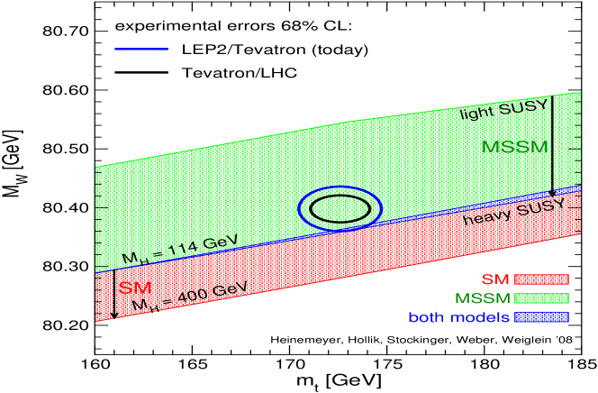
\begin{picture}(0.0,0.0) \put(0.0,0.0){} \put(0.0,0.0){} \end{picture}

Figure 1: Prediction for $M_{W}$ in the MSSM and the SM (see text) as a function of $m_{t}$ in comparison with the present experimental results for $M_{W}$ and $m_{t}$ [41].

The current 68% C.L. experimental results and their LHC expectations for $m_{t}$ and $M_{W}$ are indicated in the plot as blue and black ellipses, respectively. As can be seen from Fig. 1, the current experimental 68% C.L. region for $m_{t}$ and $M_{W}$ exhibits a slight preference of the MSSM over the SM. At the 95% C.L. (not shown) the current experimental values enter the SM parameter space. This example indicates that the experimental measurement of $M_{W}$ in combination with $m_{t}$ prefers within the SM a relatively small value of $M_{H}^{\mathrm{SM}}$, or with the MSSM not too heavy SUSY mass scales. A fit to all electroweak precision observables (EWPO) (including $M_{W}$ and $m_{t}$) determines $M_{H}^{\mathrm{SM}}$ currently to $\sim 36\%$ [17],

$$M_{H}^{\mathrm{SM}}=87^{+36}_{-27}\,\,\mathrm{GeV}.$$ (4)

This is shown in the “blue band” plot in Fig. 2 [17]. In this figure $\Delta\chi^{2}$ is shown as a function of $M_{H}^{\mathrm{SM}}$, yielding Eq. (4) as best fit with an upper limit of $160\,\,\mathrm{GeV}$ at 95% C.L. This value increases to $190\,\,\mathrm{GeV}$ if the direct LEP bound of $114.4\,\,\mathrm{GeV}$ at the 95% C.L. [48] is included in the fit. The theory (intrinsic) uncertainty in the SM calculations (as evaluated with TOPAZ0 [52] and ZFITTER [53]) are represented by the thickness of the blue band. The width of the parabola itself, on the other hand, is determined by the experimental precision of the measurements of the EWPO and the input parameters.

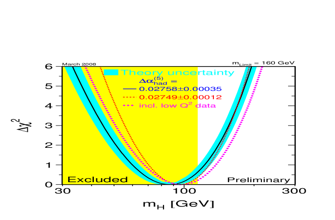
Figure 2: $\Delta\chi^{2}$ curve derived from all EWPO measured at LEP, SLD, CDF and D0, as a function of $M_{H}^{\mathrm{SM}}$, assuming the SM to be the correct theory of nature [17].

With the future improvements at the LHC in $m_{t}$ and $M_{W}$, shown as the black ellipse in Fig. 1, the precision of the indirect determination of $M_{H}^{\mathrm{SM}}$ will increase [19] as indicated in Tab. 1.

3 SM Higgs physics at the LHC

3.1 Discovering a Higgs boson

In order to “discover the Higgs boson” several steps have to be taken, as summarized in Tab. 2. Simply detecting a new particle and measure its mass (and checking whether it is in agreement with the model predictions, see e.g. the last line of Tab. 1) is not sufficient. In order to establish the Higgs mechanism the coupling of the new state to fermions and gauge bosons has to be measured and compared with the model predictions. Finally also the self-coupling (corresponding to the Higgs potential) as well as its spin and quantum numbers have to be determined experimentally. Only if all measurements agree with the prediction of the Higgs mechanism (of e.g. the SM) “discovery of the Higgs boson” can be claimed.

Finding a Higgs candidate particle and providing a rough mass measurement might still be possible at the Tevatron (depending somewhat on its mass) [7]. The discovery of a SM-like Higgs is guaranteed at the LHC, where also a relative precise mass measurement and possibly a coarse measurement of its couplings to SM fermions and gauge bosons can be performed, see Sect. 3.2. However, the final steps for the establishment of the Higgs mechanism, measurement of the self-coupling as well as of the quantum numbers can most probably only be performed at the $e^{+}e^{-}$ ILC [10, 11, 12, 54]. The anticipated capabilities of the various colliders are summarized in Tab. 2.

1. Find the new particle	T	L	I
2. measure its mass ($\Rightarrow$ ok?)	T	L	I
3. measure coupling to gauge bosons		L	I
4. measure couplings to fermions		L	I
5. measure self-couplings			I
6. measure spin, …			I

Table 2: Steps that have to be taken to “discover the Higgs”. Indicated are the colliders at which a certain measurement (most likely) can be performed: T = Tevatron, L = LHC, I = ILC.

3.2 SM Higgs boson mass and couplings at the LHC

A SM-like Higgs boson can be produced in many channels at the LHC as shown in Fig. 3 (taken from Ref. [55], where also the relevant original references can be found). The corresponding discovery potential for a SM-like Higgs boson of ATLAS is shown in Fig. 4 [56], where similar results have been obtained for CMS [9]. With $10\,\mbox{fb}^{-1}$ a $5\,\sigma$ discovery is expected for $M_{H}^{\mathrm{SM}}\;\raisebox{-3.00003pt}{$\stackrel{{\scriptstyle\displaystyle>}}{{\sim}}$}\;130\,\,\mathrm{GeV}$. For lower masses a higher integrated luminosity will be needed. The largest production cross section is reached by $gg\to H$, which however, will be visible only in the decay to SM gauge bosons. A precise mass measurement of $M_{h}^{\rm exp}\approx 200\,\,\mathrm{MeV}$ can be provided by the decays $H\to\gamma\gamma$ at lower Higgs masses and by $H\to ZZ^{(*)}\to 4\ell$ at higher masses. This guarantees the detection of the new state and a precise mass measurement over the relevant parameter space within the SM.

The next step will be the determination of the Higgs boson couplings to SM fermions and gauge bosons. We will focus here on the analysis presented in Ref. [57]. As shown in Fig. 3, the LHC will provide us with many different Higgs observation channels. In the SM there are four relevant production modes: gluon fusion (GF; loop-mediated, dominated by the top quark), which dominates inclusive production; weak boson fusion (WBF), which has an additional pair of hard and far-forward/backward jets in the final state; top-quark associated production ($t\bar{t}H$); and weak boson associated production ($WH,ZH$), where the weak boson is identified by its leptonic decay. In general, the LHC will be able to observe Higgs decays to photons, weak bosons, tau leptons and $b$ quarks, in the range of Higgs masses where the branching ratio (BR) in question is not too small.

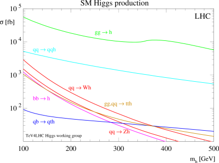
Figure 3: The various production cross sections for a SM-like Higgs boson at the LHC are shown as a function of $M_{H}^{\mathrm{SM}}$ (taken from Ref. [55], where also the relevant references can be found).

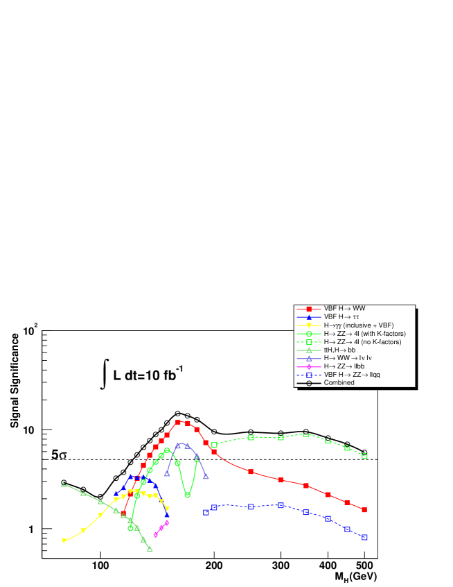
Figure 4: Significance of a Higgs signal, measured at ATLAS with $10\,\mbox{fb}^{-1}$ [56]. Similar results have been obtained for CMS [9].

For a Higgs in the intermediate mass range, the total width, $\Gamma$, is expected to be small enough to use the narrow-width approximation in extracting couplings. The rate of any channel (with the $H$ decaying to final state particles $xx$) is, to a good approximation, given by

$$\sigma(H)\times{\rm BR}(H\to xx)={\sigma(H)^{\rm SM}\over\Gamma_{p}^{\rm SM}}\cdot{\Gamma_{p}\Gamma_{x}\over\Gamma}\;,$$ (5)

where $\Gamma_{p}$ is the Higgs partial width involving the production couplings, and where the Higgs branching ratio for the decay is written as ${\rm BR}(H\to xx)=\Gamma_{x}/\Gamma$. Even with cuts, the observed rate directly determines the product $\Gamma_{p}\Gamma_{x}/\Gamma$ (normalized to the calculable SM value of this product). The LHC will have access to (or provide upper limits on) combinations of $\Gamma_{g},\Gamma_{W},\Gamma_{Z},\Gamma_{\gamma},\Gamma_{\tau},\Gamma_{b}$ and the square of the top Yukawa coupling, $Y_{t}$. The analysis of Ref. [57] was based on the channels: GF $gg\rightarrow H\rightarrow ZZ$, WBF $qq\,H\rightarrow qq\,ZZ$, GF $gg\rightarrow H\rightarrow WW$, WBF $qq\,H\rightarrow qq\,WW$, $W\,H\rightarrow W\,WW$ (2$l$ and 3$l$ final state), $t\bar{t}\,H(H\rightarrow WW,t\rightarrow Wb)$ (2$l$ and 3$l$ final state), inclusive Higgs boson production: $H\rightarrow\gamma\gamma$, WBF $qq\,H\rightarrow qq\,\gamma\gamma$, $t\bar{t}\,H(H\rightarrow\gamma\gamma)$, $W\,H(H\rightarrow\gamma\gamma)$, $Z\,H(H\rightarrow\gamma\gamma)$, WBF $qq\,H\rightarrow qq\,\tau\tau$, $t\bar{t}\,H(H\rightarrow b\bar{b})$. The significance of the last channel has become substantially worse in the recent ATLAS and CMS analyses [56, 9] (also the other channels have been re-analyzed in the recent years). This should be kept in mind for the results reviewed here. They might become worse in an updated analysis.

The production and decay channels listed above refer to a single Higgs resonance, with decay signatures which also exist in the SM. The Higgs sector may be much richer, of course, see e.g. Sect. 4. However, no analysis has yet been performed for a non-SM-like Higgs scenario.

While from the channels listed above ratios of couplings (or partial widths) can be extracted in a fairly model-independent way, see e.g. Ref. [58], further theoretical assumptions are necessary in order to determine absolute values of the Higgs couplings to fermions and bosons and of the total Higgs boson width. The only assumption that was used in Ref. [57] is that the strength of the Higgs–gauge-boson couplings does not exceed the SM value by more than 5%

$$\Gamma_{V}\leq\Gamma_{V}^{\rm SM}\times 1.05,\quad V=W,Z~{}.$$ (6)

This assumption is justified in any model with an arbitrary number of Higgs doublets (with or without additional Higgs singlets), i.e., it is true for the MSSM in particular. While Eq. (6) constitutes an upper bound on the Higgs coupling to weak bosons, the mere observation of Higgs production puts a lower bound on the production couplings and, thereby, on the total Higgs width. The constraint $\Gamma_{V}\leq\Gamma_{V}^{\rm SM}\times 1.05$, combined with a measurement of $\Gamma_{V}^{2}/\Gamma$ from observation of $H\to VV$ in WBF, then puts an upper bound on the Higgs total width, $\Gamma$. Thus, an absolute determination of the Higgs total width is possible in this way. Using this result, an absolute determination also becomes possible for Higgs couplings to gauge bosons and fermions.

The expected LHC accuracies are obtained from a $\chi^{2}$ fit based on experimental information for the channels listed above. Details on the fitting procedure, error assumptions etc. can be found in Ref. [57]. The results below are shown for two luminosity assumptions for the LHC:
30 fb^-1 at each of two experiments, denoted $2\times 30$ fb^-1;
300 fb^-1 at each of two experiments, of which only 100 fb^-1 is usable for WBF channels at each experiment, denoted $2\times 300$ $+$ $2\times 100$ fb^-1;
The latter case allows for possible significant degradation of the WBF channels in a high luminosity environment.

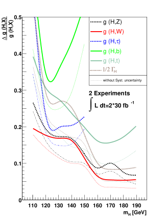
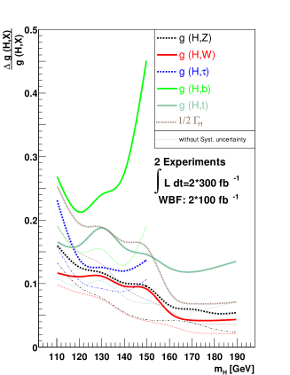
Figure 5: Precision for various Higgs boson couplings based on Ref. [57] as a function of the Higgs boson mass. The left plot assumes $30\,\mbox{fb}^{-1}$ at each of the two experiments, the right plot assumes $300\,\mbox{fb}^{-1}$ at each experiment, where, however, only $100\,\mbox{fb}^{-1}$ can be used in the WBF channel. The thin lines show the result without systematic uncertainties.

The results of the fit for the Higgs boson couplings are shown in Fig. 5 as a function of the SM Higgs boson mass. The left plot contains the results for the low luminosity case. Couplings to gauge bosons can be determined at the level of $\sim 20\%$ for $M_{H}^{\mathrm{SM}}\;\raisebox{-3.00003pt}{$\stackrel{{\scriptstyle\displaystyle<}}{{\sim}}$}\;150\,\,\mathrm{GeV}$ and at 5–10% for higher Higgs boson masses. For the couplings to SM fermions the fit yields a precision between 20 and 40% depending on the fermion species and $M_{H}^{\mathrm{SM}}$. Above $M_{H}^{\mathrm{SM}}\approx 150\,\,\mathrm{GeV}$ the only fermion coupling that can be determined is the one to the top quark. The accuracies of the coupling determination improve substantially for the high luminosity case as shown in the right plot of Fig. 5. Couplings to the SM gauge bosons are fitted with a precision of 5–10% for all $M_{H}^{\mathrm{SM}}$, and the couplings to fermions are measured a the 15–25% level.

As mentioned above, taking recent experimental analyses on the various Higgs production and decay channels into account [56, 9], the results could change. Furthermore there might be some chances to measure the spin, the ${\cal CP}$ properties and the $HVV$ vertex structure of the Higgs bosons for $M_{H}^{\mathrm{SM}}\;\raisebox{-3.00003pt}{$\stackrel{{\scriptstyle\displaystyle>}}{{\sim}}$}\;160\,\,\mathrm{GeV}$ [59]. However, within the SM this mass range is disfavored by the electroweak precision data, see Sect. 2.

4 MSSM Higgs bosons at the LHC

In this section we focus on the MSSM with real parameters. Contrary to the Standard Model (SM), in the MSSM two Higgs doublets are required. The Higgs potential

$$V = m_{1}^{2}|{\cal H}_{1}|^{2}+m_{2}^{2}|{\cal H}_{2}|^{2}-m_{12}^{2}(\epsilon_{ab}{\cal H}_{1}^{a}{\cal H}_{2}^{b}+\mbox{h.c.})$$ (7)

$$+\frac{1}{8}(g_{1}^{2}+g_{2}^{2})\left[|{\cal H}_{1}|^{2}-|{\cal H}_{2}|^{2}\right]^{2}+\frac{1}{2}g_{2}^{2}|{\cal H}_{1}^{{\dagger}}{\cal H}_{2}|^{2}~{},$$

contains $m_{1},m_{2},m_{12}$ as soft SUSY breaking parameters; $g_{2},g_{1}$ are the $SU(2)$ and $U(1)$ gauge couplings, and $\epsilon_{12}=-1$.

The doublet fields $H_{1}$ and $H_{2}$ are decomposed in the following way:

$${\cal H}_{1} = \left(\begin{array}[]{c}{\cal H}_{1}^{0}\\[2.15277pt] {\cal H}_{1}^{-}\end{array}\right)\;=\;\left(\begin{array}[]{c}v_{1}+\frac{1}{\sqrt{2}}(\phi_{1}^{0}-i\chi_{1}^{0})\\[2.15277pt] -\phi_{1}^{-}\end{array}\right)~{},$$ (12)

$${\cal H}_{2} = \left(\begin{array}[]{c}{\cal H}_{2}^{+}\\[2.15277pt] {\cal H}_{2}^{0}\end{array}\right)\;=\;\left(\begin{array}[]{c}\phi_{2}^{+}\\[2.15277pt] v_{2}+\frac{1}{\sqrt{2}}(\phi_{2}^{0}+i\chi_{2}^{0})\end{array}\right)~{}.$$ (17)

The potential (7) can be described with the help of two independent parameters (besides $g_{2}$ and $g_{1}$): $\tan\beta=v_{2}/v_{1}$ and $M_{A}^{2}=-m_{12}^{2}(\tan\beta+\cot\beta)$, where $M_{A}$ is the mass of the ${\cal CP}$-odd Higgs boson $A$.

The diagonalization of the bilinear part of the Higgs potential, i.e. of the Higgs mass matrices, is performed via the orthogonal transformations

$$\left(\begin{array}[]{c}H^{0}\\[2.15277pt] h^{0}\end{array}\right) = \left(\begin{array}[]{cc}\cos\alpha&\sin\alpha\\[2.15277pt] -\sin\alpha&\cos\alpha\end{array}\right)\left(\begin{array}[]{c}\phi_{1}^{0}\\[2.15277pt] \phi_{2}^{0}~{},\end{array}\right)$$ (24)

$$\left(\begin{array}[]{c}G^{0}\\[2.15277pt] A^{0}\end{array}\right) = \left(\begin{array}[]{cc}\cos\beta&\sin\beta\\[2.15277pt] -\sin\beta&\cos\beta\end{array}\right)\left(\begin{array}[]{c}\chi_{1}^{0}\\[2.15277pt] \chi_{2}^{0}\end{array}\right)~{},$$ (31)

$$\left(\begin{array}[]{c}G^{\pm}\\[2.15277pt] H^{\pm}\end{array}\right) = \left(\begin{array}[]{cc}\cos\beta&\sin\beta\\[2.15277pt] -\sin\beta&\cos\beta\end{array}\right)\left(\begin{array}[]{c}\phi_{1}^{\pm}\\[2.15277pt] \phi_{2}^{\pm}\end{array}\right)~{}.$$ (38)

The mixing angle $\alpha$ is determined through

$$\alpha={\rm arctan}\left[\frac{-(M_{A}^{2}+M_{Z}^{2})\sin\beta\cos\beta}{M_{Z}^{2}\cos^{2}\beta+M_{A}^{2}\sin^{2}\beta-m^{2}_{h,{\rm tree}}}\right]~{},~{}~{}-\frac{\pi}{2}<\alpha<0~{}.$$ (39)

One gets the following Higgs spectrum:

$$\mbox{2 neutral bosons},\,{\cal CP}=+1 : h,H$$

$$\mbox{1 neutral boson},\,{\cal CP}=-1 : A$$

2 charged bosons $$: H^{+},H^{-}$$

3 unphysical Goldstone bosons $$: G,G^{+},G^{-}.$$ (40)

Since the MSSM Higgs boson sector at tree-level can be described with $M_{A}$ and $\tan\beta$, all other masses and mixing angles are predicted. These tree-level relations receive large higher-order corrections, see e.g. Refs. [47, 60, 61] for reviews. A typical mass spectrum (including higher-order corrections, obtained with the Fortran code FeynHiggs [50, 51, 62, 63]) is shown in Fig. 6. The Higgs masses are shown as a function of $M_{A}$ for $\tan\beta$ in the $m_{h}^{\rm max}$ benchmark scenario [64]. At low $M_{A}$ the lightest Higgs boson mass rises, until at around $M_{A}\approx 200\,\,\mathrm{GeV}$ a maximum and plateau is reached. This is the so-called “decoupling” limit. Here the lightest Higgs is SM-like, while all the masses of the heavy Higgses are very close to each other.

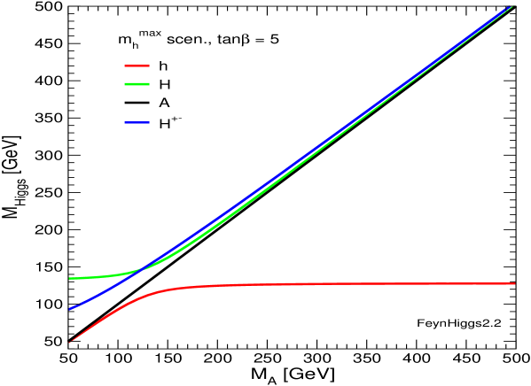
Figure 6: The MSSM Higgs boson masses (including higher-order corrections) are shown as a function of $M_{A}$ for $\tan\beta=5$ in the $m_{h}^{\rm max}$ benchmark scenario [64].

The couplings of the MSSM Higgs bosons differ already at the tree-level from the corresponding SM couplings. Some couplings important for the Higgs boson phenomenology are given by

$$g_{hVV} =\sin(\beta-\alpha)\;g_{HVV}^{\rm SM},\quad V=W^{\pm},Z,$$ (41)

$$g_{HVV} =\cos(\beta-\alpha)\;g_{HVV}^{\rm SM},$$ (42)

$$g_{hb\bar{b}},g_{h\tau^{+}\tau^{-}} =-\sin\alpha/\cos\beta\;g_{Hb\bar{b},H\tau^{+}\tau^{-}}^{\rm SM},$$ (43)

$$g_{ht\bar{t}} =\cos\alpha/\sin\beta\;g_{Ht\bar{t}}^{\rm SM},$$ (44)

$$g_{Ab\bar{b}},g_{A\tau^{+}\tau^{-}} =\gamma_{5}\tan\beta\;g_{Hb\bar{b}}^{\rm SM}.$$ (45)

The couplings of the neutral ${\cal CP}$-even Higgs bosons to gauge bosons is always suppressed. However, not all of the couplings can be made small simultaneously. The coupling of the light Higgs boson to down-type fermions (especially to bottom quarks and tau leptons) can be enhanced at large $\tan\beta$. In the decoupling limit one finds in $\beta-\alpha\to\pi/2$ and specifically $g_{hxx}\to g_{Hxx}^{\mathrm{SM}}$. On the other hand, the coupling of the ${\cal CP}$-odd Higgs boson to down-type fermions is always enhanced by $\tan\beta$.

The resulting LHC production cross sections are shown in Fig. 7 [55]. They are given as a function of $M_{A}$ for $\tan\beta=5$ in the $m_{h}^{\rm max}$ benchmark scenario. The most striking difference in comparison with the SM is the appearance of the $b\bar{b}\phi$ ($\phi=h,H,A$) channel. Due to the possible enhancement in the MSSM, see Eqs. (43), (45), this cross section can yield a detectable signal.

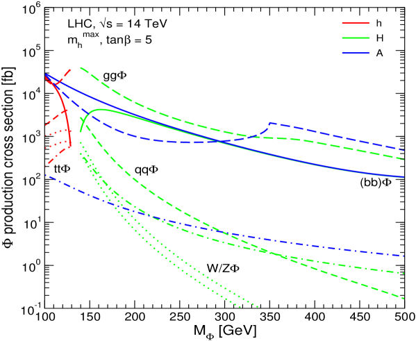
Figure 7: Overview about the various neutral Higgs boson production cross sections at the LHC shown as a function of $M_{A}$ for $\tan\beta=5$ in the $m_{h}^{\rm max}$ scenario (taken from Ref. [55], where the original references can be found).

4.1 The light MSSM Higgs boson

The mass of the lightest MSSM Higgs boson mass is bounded from above by $M_{Z}$ at the tree-level. Including loop corrections this bound is pushed upwards to $M_{h}\;\raisebox{-3.00003pt}{$\stackrel{{\scriptstyle\displaystyle<}}{{\sim}}$}\;135\,\,\mathrm{GeV}$ (as obtained with FeynHiggs). This bound includes already the parametric uncertainty from the top-quark mass, see Eq. (1), and the theory uncertainty due to unknown higher-order corrections [51, 47]. This bound makes a firm prediction for the searches at the LHC.

Alternatively, $M_{h}$ can be determined in a global fit to the EWPO, similar to the result shown in Fig. 2. The corresponding result for $M_{h}$ in the Constrained MSSM (CMSSM) has been obtained in Ref. [65]. Furthermore included in the fit are the anomalous magnetic moment of the muon, the B-physics observables ${\rm BR}(b\to s\gamma)$ and ${\rm BR}(B_{s}\to\mu^{+}\mu^{-})$ as well as the prediction for the Cold Dark Matter abundance, see Ref. [65] for all the relevant references. This yields (using $m_{t}^{\rm exp}=170.9\pm 1.8\,\,\mathrm{GeV}$)

$$M_{h}^{\rm CMSSM}=110^{+10}_{-8}\pm 3\,\,\mathrm{GeV},$$ (46)

where the first error is experimental and the second one due to unknown higher-order corrections [51, 47]. This has to be compared to Eq. (4) and to the bounds on the Higgs boson masses obtained at LEP, $114.4\,\,\mathrm{GeV}$ at the 95% C.L. [48], which is valid also in the CMSSM [66, 67]. Despite its simplicity, the $M_{h}$ prediction in the CMSSM is in better agreement with the LEP bounds than the SM.

Within the decoupling limit, $M_{A}\;\raisebox{-3.00003pt}{$\stackrel{{\scriptstyle\displaystyle>}}{{\sim}}$}\;200\,\,\mathrm{GeV}$, the lightest MSSM Higgs is SM-like. Its production and decay and consequently its detection can proceed via the SM channels. However, two possible deviations from the SM case should be kept in mind. First, the $gg\to h$ cross section can be strongly suppressed due to additional scalar top loops [68]. This is realized in the “gluophobic Higgs” benchmark scenario [64]. In this case for $M_{A}\;\raisebox{-3.00003pt}{$\stackrel{{\scriptstyle\displaystyle<}}{{\sim}}$}\;400\,\,\mathrm{GeV}$ a suppression of the $gg\to h$ production cross section by more than 60% as compared to the SM cross section takes place. Second, the decay $h\to\gamma\gamma$ can be suppressed due to an enhanced $hb\bar{b}$ coupling. This could hamper the precise measurement of $M_{h}$, which proceeds via the decay to photons for $M_{h}\;\raisebox{-3.00003pt}{$\stackrel{{\scriptstyle\displaystyle<}}{{\sim}}$}\;130\,\,\mathrm{GeV}$. As an example, with $30\,\mbox{fb}^{-1}$ in the $m_{h}^{\rm max}$ scenario a precise mass measurement will only be possible for $M_{A}\;\raisebox{-3.00003pt}{$\stackrel{{\scriptstyle\displaystyle>}}{{\sim}}$}\;300\,\,\mathrm{GeV}$ [9].

4.2 The heavy MSSM Higgs bosons

The main channel to discover the heavy neutral Higgs bosons for
$M_{A}\;\raisebox{-3.00003pt}{$\stackrel{{\scriptstyle\displaystyle>}}{{\sim}}$}\;200\,\,\mathrm{GeV}$ is the production in association with bottom quarks and the subsequent decay to tau leptons, $b\bar{b}\to b\bar{b}\;H/A\to b\bar{b}\;\tau^{+}\tau^{-}$. For heavy supersymmetric particles, with masses far above the Higgs boson mass scale, one has for the production and decay of the $A$ boson [69]

$$\sigma(b\bar{b}A)\times{\rm BR}(A\to b\bar{b})\simeq\sigma(b\bar{b}H)_{\rm SM}\;\frac{\tan^{2}\beta}{\left(1+\Delta_{b}\right)^{2}}\times\frac{9}{\left(1+\Delta_{b}\right)^{2}+9}~{},$$ (47)

$$\sigma(gg,b\bar{b}\to A)\times{\rm BR}(A\to\tau^{+}\tau^{-})\simeq\sigma(gg,b\bar{b}\to H)_{\rm SM}\;\frac{\tan^{2}\beta}{\left(1+\Delta_{b}\right)^{2}+9}~{},$$ (48)

where $\sigma(b\bar{b}H)_{\rm SM}$ and $\sigma(gg,b\bar{b}\to H)_{\rm SM}$ denote the values of the corresponding SM Higgs boson production cross sections for $M_{H}^{\mathrm{SM}}=M_{A}$. $\Delta_{b}$ is given by [70]

$$\Delta_{b}=\frac{2\alpha_{s}}{3\,\pi}\,m_{\tilde{g}}\,\mu\,\tan\beta\,\times\,I(m_{\tilde{b}_{1}},m_{\tilde{b}_{2}},m_{\tilde{g}})+\frac{\alpha_{t}}{4\,\pi}\,A_{t}\,\mu\,\tan\beta\,\times\,I(m_{\tilde{t}_{1}},m_{\tilde{t}_{2}},\mu)~{},$$ (49)

where the function $I$ arises from the one-loop vertex diagrams and scales as $I(a,b,c)\sim 1/\mbox{max}(a^{2},b^{2},c^{2})$. Here $m_{\tilde{t}_{1}},m_{\tilde{t}_{2}}$ and $m_{\tilde{b}_{1}},m_{\tilde{b}_{2}}$ denote the two scalar top and bottom masses, respectively. $m_{\tilde{g}}$ is the gluino mass, $\mu$ is the Higgs mixing parameter, and $A_{t}$ denotes the trilinear Higgs-stop coupling. As a consequence, the $b\bar{b}$ production rate depends sensitively on $\Delta_{b}\propto\mu\,\tan\beta$ because of the factor $1/(1+\Delta_{b})^{2}$, while this leading dependence on $\Delta_{b}$ cancels out in the $\tau^{+}\tau^{-}$ production rate. The formulas above apply, within a good approximation, also to the heavy ${\cal CP}$-even Higgs boson in the large $\tan\beta$ regime. Therefore, the production and decay rates of $H$ are governed by similar formulas as the ones given above, leading to an approximate enhancement by a factor 2 of the production rates with respect to the ones that would be obtained in the case of the single production of the ${\cal CP}$-odd Higgs boson as given in Eqs. (47), (48).

Of particular interest is the “LHC wedge” region, i.e. the region in which only the light ${\cal CP}$-even MSSM Higgs boson, but non of the heavy MSSM Higgs bosons can be detected at the LHC at the 5$\,\sigma$ level. It appears for $M_{A}\;\raisebox{-3.00003pt}{$\stackrel{{\scriptstyle\displaystyle>}}{{\sim}}$}\;200\,\,\mathrm{GeV}$ at intermediate $\tan\beta$ and widens to larger $\tan\beta$ values for larger $M_{A}$. Consequently, in the “LHC wedge” only a SM-like light Higgs boson can be discovered at the LHC. This region is bounded from above by the $5\,\sigma$ discovery contours for the heavy neutral MSSM Higgs bosons as described above. These discovery contours depend sensitively on the Higgs mass parameter $\mu$. The dependence on $\mu$ enters in two different ways, on the one hand via higher-order corrections through $\Delta_{b}\propto\mu\,\tan\beta$, and on the other hand via the kinematics of Higgs decays into charginos and neutralinos, where $\mu$ enters in their respective mass matrices [2].

In Fig. 8 we show the $5\,\sigma$ discovery regions for the heavy neutral MSSM Higgs bosons in the channel $b\bar{b}\to b\bar{b}\;H/A,H/A\to\tau^{+}\tau^{-}\to\mbox{jets}$ [71]. As explained above, these discovery contours correspond to the upper bound of the “LHC wedge”. A strong variation with the sign and the size of $\mu$ can be observed and should be taken into account in experimental and phenomenological analyses. The same higher-order corrections are relevant once a possible heavy Higgs boson signal at the LHC will be interpreted in terms of the underlying parameter space. From Eq. (49) it follows that an observed production cross section can be correctly connected to $\mu$ and $\tan\beta$ only if the scalar top and bottom masses, the gluino mass and the trilinear Higgs-stop coupling are measured and taken properly into account.

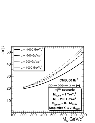
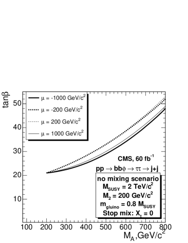
Figure 8: The $5\,\sigma$ discovery regions (i.e. the upper bound of the “LHC wedge” region) for the heavy neutral Higgs bosons in the channel $b\bar{b}\to b\bar{b}\;H/A,H/A\to\tau^{+}\tau^{-}\to\mbox{jets}$ (taken from Ref. [71]).

References

- [1] S. Glashow, Nucl. Phys. 22 (1961) 579; S. Weinberg, Phys. Rev. Lett. 19 (1967) 19; A. Salam, in: Proceedings of the 8th Nobel Symposium, Editor N. Svartholm, Stockholm, 1968.
- [2] H. Nilles, Phys. Rept. 110 (1984) 1; H. Haber and G. Kane, Phys. Rept. 117 (1985) 75; R. Barbieri, Riv. Nuovo Cim. 11 (1988) 1.
- [3] J. Gunion, H. Haber, G. Kane and S. Dawson, The Higgs Hunter’s Guide (Perseus Publishing, Cambridge, MA, 1990), and references therein.
- [4] N. Arkani-Hamed, A. Cohen and H. Georgi, Phys. Lett. B 513 (2001) 232 [arXiv:hep-ph/0105239]; N. Arkani-Hamed, A. Cohen, T. Gregoire and J. Wacker, JHEP 0208 (2002) 020 [arXiv:hep-ph/0202089]; for a review see: M. Schmaltz and D. Tucker-Smith, Ann. Rev. Nucl. Part. Sci. 55 (2005) 229 [arXiv:hep-ph/0502182].
- [5] N. Arkani-Hamed, S. Dimopoulos and G. Dvali, Phys. Lett. B 429 (1998) 263 [arXiv:hep-ph/9803315]; Phys. Lett. B 436 (1998) 257 [arXiv:hep-ph/9804398]; I. Antoniadis, Phys. Lett. B 246 (1990) 377; J. Lykken, Phys. Rev. D 54 (1996) 3693 [arXiv:hep-th/9603133]; I. Antoniadis and M. Quiros, Phys. Lett. B 392 (1997) 61 [arXiv:hep-th/9609209]; L. Randall and R. Sundrum, Phys. Rev. Lett. 83 (1999) 3370 [arXiv:hep-ph/9905221]; for reviews see: J. Hewett and M. Spiropulu, Ann. Rev. Nucl. Part. Sci. 52 (2002) 397 [arXiv:hep-ph/0205106]; T. Rizzo, arXiv:hep-ph/0409309; C. Csaki, J. Hubisz and P. Meade, arXiv:hep-ph/0510275.
- [6] W. Yao et al. [Particle Data Group Collaboration], J. Phys. G 33 (2006) 1.
- [7] See: www-cdf.fnal.gov/physics/projections/ .
-
[8]
ATLAS Collaboration,
Detector and Physics Performance Technical Design Report,
CERN/LHCC/99-15 (1999), see:
atlasinfo.cern.ch/Atlas/GROUPS/PHYSICS/TDR/access.html . - [9] CMS Collaboration, CMS Physics Technical Design Report, Volume 2. CERN/LHCC 2006-021, see: cmsdoc.cern.ch/cms/cpt/tdr/ .
- [10] J. Aguilar-Saavedra et al., TESLA TDR Part 3: “Physics at an Linear Collider” [arXiv:hep-ph/0106315], see: tesla.desy.de/tdr/ ; K. Ackermann et al., DESY-PROC-2004-01.
- [11] T. Abe et al. [American Linear Collider Working Group Collaboration], Resource book for Snowmass 2001, arXiv:hep-ex/0106055; arXiv:hep-ex/0106056; arXiv:hep-ex/0106057.
- [12] K. Abe et al. [ACFA Linear Collider Working Group Collaboration], arXiv:hep-ph/0109166.
- [13] G. Weiglein et al. [LHC/ILC Study Group], Phys. Rept. 426 (2006) 47 [arXiv:hep-ph/0410364].
- [14] Tevatron Electroweak Working Group, axXiv:0803.1683 [hep-ex].
- [15] Tevatron Electroweak Working Group, see: tevewwg.fnal.gov .
- [16] S. Moch and P. Uwer, arXiv:0804.1476 [hep-ph]; M. Cacciari, S. Frixione, M. Mangano, P. Nason and G. Ridolfi, arXiv:0804.2800 [hep-ph]; N. Kidonakis and R. Vogt, arXiv:0805.3844 [hep-ph].
-
[17]
LEP Electroweak Working Group,
see:
lepewwg.web.cern.ch/LEPEWWG/Welcome.html . - [18] T. Aaltonen et al. [CDF Collaboration], arXiv:0707.0085 [hep-ex].
- [19] M. Grünewald, arXiv:0709.3744 [hep-ex]; arXiv:0710.2838 [hep-ex].
- [20] S. Brensing, S. Dittmaier, M. Krämer and A. Mück, Phys. Rev. D 77 (2008) 073006 [arXiv:0710.3309 [hep-ph]].
- [21] M. Grünewald et al., arXiv:hep-ph/0005309.
- [22] The ALEPH, DELPHI, L3, OPAL, SLD Collaborations, the LEP Electroweak Working Group, the SLD Electroweak and Heavy Flavour Groups, Phys. Rept. 427 (2006) 257 [arXiv:hep-ex/0509008]; [The ALEPH, DELPHI, L3 and OPAL Collaborations, the LEP Electroweak Working Group], arXiv:hep-ex/0612034.
- [23] A. Denner, S. Dittmaier, M. Roth and D. Wackeroth, Nucl. Phys. 560 (1999) 33 [arXiv:hep-ph/9904472]; Nucl. Phys. B 587 (2000) 67 [arXiv:hep-ph/0006307]; Comput. Phys. Commun. 153 (2003) 462 [arXiv:hep-ph/0209330].
- [24] S. Jadach, W. Placzek, M. Skrzypek, B. Ward and Z. Was, Phys. Rev. D 65 (2002) 093010 [arXiv:hep-ph/0007012]; Comput. Phys. Commun. 140 (2001) 432 [arXiv:hep-ph/0103163].
- [25] C. Balazs and C. P. Yuan, Phys. Rev. 56 (1997) 5558 [arXiv:hep-ph/9704258].
- [26] U. Baur, S. Keller and D. Wackeroth, Phys. Rev. D 59 (1999) 013002 [arXiv:hep-ph/9807417].
- [27] U. Baur, R. Clare, J. Erler, S. Heinemeyer, D. Wackeroth, G. Weiglein and D. Wood, arXiv:hep-ph/0111314.
- [28] S. Heinemeyer, T. Mannel and G. Weiglein, arXiv:hep-ph/9909538; J. Erler, S. Heinemeyer, W. Hollik, G. Weiglein and P. Zerwas, Phys. Lett. B 486 (2000) 125 [arXiv:hep-ph/0005024].
- [29] R. Hawkings and K. Mönig, EPJdirect C8 (1999) 1 [arXiv:hep-ex/9910022].
- [30] G. Wilson, LC-PHSM-2001-009, see: www.desy.de/lcnotes/notes.html .
- [31] A. Sirlin, Phys. Rev. D 22 (1980) 971; W. Marciano and A. Sirlin, Phys. Rev. D 22 (1980) 2695.
- [32] A. Freitas, W. Hollik, W. Walter and G. Weiglein, Phys. Lett. B 495 (2000) 338 [Erratum-ibid. B 570 (2003) 260] [arXiv:hep-ph/0007091]; Nucl. Phys. B 632 (2002) 189 [Erratum-ibid. B 666 (2003) 305] [arXiv:hep-ph/0202131]; M. Awramik and M. Czakon, Phys. Lett. B 568 (2003) 48, [arXiv:hep-ph/0305248]; M. Awramik and M. Czakon, Phys. Rev. Lett. 89 (2002) 241801 [arXiv:hep-ph/0208113]; Nucl. Phys. Proc. Suppl. 116 (2003) 238 [arXiv:hep-ph/0211041]; A. Onishchenko and O. Veretin, Phys. Lett. B 551 (2003) 111 [arXiv:hep-ph/0209010]; M. Awramik, M. Czakon, A. Onishchenko and O. Veretin, Phys. Rev. D 68 (2003) 053004 [arXiv:hep-ph/0209084]; A. Djouadi and C. Verzegnassi, Phys. Lett. B 195 (1987) 265; A. Djouadi, Nuovo Cim. A 100 (1988) 357; B. Kniehl, Nucl. Phys. B 347 (1990) 89; F. Halzen and B. Kniehl, Nucl. Phys. B 353 (1991) 567; B. Kniehl and A. Sirlin, Nucl. Phys. B 371 (1992) 141; Phys. Rev. D 47 (1993) 883; A. Djouadi and P. Gambino, Phys. Rev. D 49 (1994) 3499 [Erratum-ibid. D 53 (1994) 4111] [arXiv:hep-ph/9309298].
- [33] M. Awramik, M. Czakon, A. Freitas and G. Weiglein, Phys. Rev. D 69 (2004) 053006 [arXiv:hep-ph/0311148].
- [34] L. Avdeev et al., Phys. Lett. B 336 (1994) 560 [Erratum-ibid. B 349 (1995) 597] [arXiv:hep-ph/9406363]; K. Chetyrkin, J. Kühn and M. Steinhauser, Phys. Lett. B 351 (1995) 331 [arXiv:hep-ph/9502291]; Nucl. Phys. B 482 (1996) 213 [arXiv:hep-ph/9606230].
- [35] K. Chetyrkin, J. Kühn and M. Steinhauser, Phys. Rev. Lett. 75 (1995) 3394 [arXiv:hep-ph/9504413].
- [36] M. Veltman, Nucl. Phys. B 123 (1977) 89.
- [37] J. van der Bij, K. Chetyrkin, M. Faisst, G. Jikia and T. Seidensticker, Phys. Lett. B 498 (2001) 156 [arXiv:hep-ph/0011373].
- [38] M. Faisst, J. Kühn, T. Seidensticker and O. Veretin, Nucl. Phys. B 665 (2003) 649 [arXiv:hep-ph/0302275].
- [39] R. Boughezal, J. Tausk and J. van der Bij, Nucl. Phys. B 713 (2005) 278 [arXiv:hep-ph/0410216].
- [40] Y. Schröder and M. Steinhauser, Phys. Lett. B 622 (2005) 124 [arXiv:hep-ph/0504055]; K. Chetyrkin, M. Faisst, J. Kühn, P. Maierhofer and C. Sturm, Phys. Rev. Lett. 97 (2006) 102003 [arXiv:hep-ph/0605201]; R. Boughezal and M. Czakon, Nucl. Phys. B 755 (2006) 221 [arXiv:hep-ph/0606232].
- [41] S. Heinemeyer, W. Hollik, D. Stöckinger, A.M. Weber and G. Weiglein, JHEP 08 (2006) 052 [arXiv:hep-ph/0604147].
- [42] P. Chankowski, A. Dabelstein, W. Hollik, W. Mösle, S. Pokorski and J. Rosiek, Nucl. Phys. B 417 (1994) 101.
- [43] D. Garcia and J. Solà, Mod. Phys. Lett. A 9 (1994) 211.
- [44] A. Djouadi, P. Gambino, S. Heinemeyer, W. Hollik, C. Jünger and G. Weiglein, Phys. Rev. Lett. 78 (1997) 3626 [arXiv:hep-ph/9612363]; Phys. Rev. D 57 (1998) 4179 [arXiv:hep-ph/9710438].
- [45] S. Heinemeyer and G. Weiglein, JHEP 0210 (2002) 072 [arXiv:hep-ph/0209305]; arXiv:hep-ph/0301062.
- [46] J. Haestier, S. Heinemeyer, D. Stöckinger and G. Weiglein, JHEP 0512 (2005) 027 [arXiv:hep-ph/0508139]; arXiv:hep-ph/0506259.
- [47] S. Heinemeyer, W. Hollik and G. Weiglein, Phys. Rept. 425 (2006) 265 [arXiv:hep-ph/0412214].
- [48] LEP Higgs working group, Phys. Lett. B 565 (2003) 61 [arXiv:hep-ex/0306033].
- [49] LEP Higgs working group, Eur. Phys. J. C 47 (2006) 547 [arXiv:hep-ex/0602042].
- [50] S. Heinemeyer, W. Hollik and G. Weiglein, Eur. Phys. J. C 9 (1999) 343 [arXiv:hep-ph/9812472].
- [51] G. Degrassi, S. Heinemeyer, W. Hollik, P. Slavich and G. Weiglein, Eur. Phys. J. C 28 (2003) 133 [arXiv:hep-ph/0212020].
- [52] G. Montagna, O. Nicrosini, F. Piccinini and G. Passarino, Comput. Phys. Commun. 117 (1999) 278 [arXiv:hep-ph/9804211].
- [53] D. Bardin et al., Comput. Phys. Commun. 133 (2001) 229 [arXiv:hep-ph/9908433]; A. Arbuzov et al., Comput. Phys. Commun. 174 (2006) 728 [arXiv:hep-ph/0507146].
- [54] S. Heinemeyer et al., arXiv:hep-ph/0511332.
- [55] T. Hahn, S. Heinemeyer, F. Maltoni, G. Weiglein and S. Willenbrock, arXiv:hep-ph/0607308.
- [56] See: twiki.cern.ch/twiki/bin/view/Atlas/NewHiggsCSCPage .
- [57] M. Duhrssen, S. Heinemeyer, H. Logan, D. Rainwater, G. Weiglein and D. Zeppenfeld, Phys. Rev. D 70 (2004) 113009 [arXiv:hep-ph/0406323].
- [58] M. Dührssen, ATL-PHYS-2003-030, available from cdsweb.cern.ch .
- [59] T. Plehn, D. Rainwater and D. Zeppenfeld, Phys. Rev. Lett. 88 (2002) 051801 [arXiv:hep-ph/0105325]; V. Hankele, G. Klamke, D. Zeppenfeld and T. Figy, Phys. Rev. D 74 (2006) 095001 [arXiv:hep-ph/0609075]; G. Klamke and D. Zeppenfeld, JHEP 0704 (2007) 052 [arXiv:hep-ph/0703202]; C. Ruwiedel, M. Schumacher and N. Wermes, Eur. Phys. J. C 51 (2007) 385.
- [60] S. Heinemeyer, Int. J. Mod. Phys. A 21 (2006) 2659 [arXiv:hep-ph/0407244].
- [61] A. Djouadi, Phys. Rept. 459 (2008) 1 [arXiv:hep-ph/0503173].
- [62] M. Frank, T. Hahn, S. Heinemeyer, W. Hollik, H. Rzehak and G. Weiglein, JHEP 0702 (2007) 047 [arXiv:hep-ph/0611326].
- [63] S. Heinemeyer, W. Hollik and G. Weiglein, Comput. Phys. Commun. 124 (2000) 76 [arXiv:hep-ph/9812320]; see: www.feynhiggs.de .
- [64] M. Carena, S. Heinemeyer, C. Wagner and G. Weiglein, Eur. Phys. J. C 26 (2003) 601 [arXiv:hep-ph/0202167].
- [65] O. Buchmueller et al., Phys. Lett. B 657 (2007) 87 [arXiv:0707.3447 [hep-ph]].
- [66] S. Ambrosanio, A. Dedes, S. Heinemeyer, S. Su and G. Weiglein, Nucl. Phys. B 624 (2001) 3 [arXiv:hep-ph/0106255].
- [67] J. Ellis, S. Heinemeyer, K. Olive and G. Weiglein, Phys. Lett. B 515 (2001) 348 [arXiv:hep-ph/0105061].
- [68] A. Djouadi, Phys. Lett. B 435 (1998) 101 [arXiv:hep-ph/9806315].
- [69] M. Carena, S. Heinemeyer, C. Wagner and G. Weiglein, Eur. Phys. J. C 45 (2006) 797 [arXiv:hep-ph/0511023].
- [70] R. Hempfling, Phys. Rev. D 49 (1994) 6168; L. Hall, R. Rattazzi and U. Sarid, Phys. Rev. D 50 (1994) 7048 [arXiv:hep-ph/9306309]; M. Carena, M. Olechowski, S. Pokorski and C. Wagner, Nucl. Phys. B 426 (1994) 269 [arXiv:hep-ph/9402253].
- [71] S. Gennai, S. Heinemeyer, A. Kalinowski, R. Kinnunen, S. Lehti, A. Nikitenko and G. Weiglein, Eur. Phys. J. C 52 (2007) 383 [arXiv:0704.0619 [hep-ph]]; M. Hashemi, S. Heinemeyer, R. Kinnunen, A. Nikitenko and G. Weiglein, arXiv:0804.1228 [hep-ph].