Spitzer and HHT Observations of Bok Globule B335: Isolated Star Formation Efficiency and Cloud Structure

Abstract

We present infrared and millimeter observations of Barnard 335, the prototypical isolated Bok globule with an embedded protostar. Using Spitzer data we measure the source luminosity accurately; we also constrain the density profile of the innermost globule material near the protostar using the observation of an 8.0 µm shadow. HHT observations of ¹²CO 2 – 1 confirm the detection of a flattened molecular core with diameter $\sim\!10000$ AU and the same orientation as the circumstellar disk ($\sim\!100$ to 200 AU in diameter). This structure is probably the same as that generating the 8.0 µm shadow and is expected from theoretical simulations of collapsing embedded protostars. We estimate the mass of the protostar to be only $\sim\!5$% of the mass of the parent globule.

1. Introduction

Bok & Reilly (1947) and Bok (1948) were the first to suggest that “Bok globules” could be the sites of isolated star formation. With this in mind, B$335$ (CB199 in the catalog of Clemens & Barvainis (1988)) was extensively studied in molecular lines (Martin & Barrett, 1978; Dickman, 1978) and in the far-infrared by Keene et al. (1980) and Keene (1981). Frerking & Langer (1982) discovered a “pedestal” source, i.e., a molecular outflow, indicating the possible presence of a protostar within the cloud. The presence of a protostar was quickly confirmed with additional far-infrared observations by Keene et al. (1983). Assuming a distance of 250 pc, as suggested by Tomita et al. (1979) and as adopted by most subsequent observers, Keene et al. (1983) determined the luminosity of the source within B$335$ to be about 3 L_⊙. B$335$ has subsequently been observed at far-infrared and submillimeter wavelengths by, e.g., Gee et al. (1985), Mozurkewich et al. (1986), Chandler et al. (1990), Huard et al. (1999), and Shirley et al. (2000); it is the first example of a Class 0 young stellar object to be so thoroughly studied. It is therefore the template source for many of our concepts about the early stages of the formation of low-mass stars.

Modeling has established that the globule material is still undergoing strong noncircular motions that are most likely infall (e.g., Zhou et al., 1990; Choi et al., 1995; Velusamy et al., 1995). Although this scenario of infall, and more specifically of inside-out collapse, is plausible, important discrepancies remain (e.g., Wilner et al., 2000; Harvey et al., 2001; Evans et al., 2005; Choi, 2007). Models and observations imply that the core is a star of mass $\sim\!0.5$ $\hbox{M}_{\odot}$(Zhou et al., 1990) with a circumstellar disk $\sim\!100$ to 200 AU in diameter (Harvey et al., 2003a). This source has a strong bipolar outflow (e.g., Cabrit & Bertout, 1992; Hirano et al., 1988), oriented nearly in the plane of the sky, that maintains a cavity in the interstellar medium (ISM) and is associated with the observed shocked material (Gâlfalk & Olofsson, 2007).

We describe observations with all three instruments on Spitzer and with the Heinrich Hertz Submillimeter Telescope that allow us to 1) measure the density distribution in the center of the globule; 2) constrain the geometry of the outflow and thus the protostellar disk; and 3) measure the source luminosity accurately. These measurements (with a revised distance of 150 pc) reveal a flattened molecular cloud core, consistent with numerical simulations of cloud collapse; provide tight constraints on the opening angle of the outflow; and demonstrate internal consistency between the globule luminosity (and other characteristics) and those expected for a 0.3 to 0.4 $\hbox{M}_{\odot}$ young star.

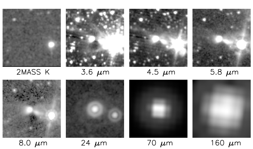
Figure 1.— Gallery of images of B335 (CB199) at the indicated wavelengths. Images are shown with a logarithmic intensity scale and are 1$\farcm$6 on a side. North is up and east is to the left.

2. Observations and processing

2.1. Spitzer data

B$335$ was observed by the Spitzer Space Telescope on 2004 April 20 and 21 with the Infrared Array Camera (IRAC; Fazio et al., 2004) AORKEYs 4926208 and 4926464; 2004 October 15 with the Multiband Imaging Photometer (MIPS; Rieke et al., 2004) AORKEY 12022106; and 2004 October 14 with the Infrared Spectrograph (IRS; Houck et al., 2004) AORKEY 3567360. Observations were made at two closely separated epochs to permit the elimination of asteroids from the final mosaic. The field of view with coverage in all four IRAC bands is $5.5\arcmin\times 13.6\arcmin$, with a larger field covered in at least two bands. For each IRAC band, 3 overlapping positions arranged along a column were imaged. At each position five small Gaussian dithers of 10.4 s duration were taken. In the region where we had coverage in all four bands, this resulted in an average exposure time of about 120 sec. For each dither, the 10.4 second long-integration frame was accompanied by a short-integration frame of 0.4s in “high dynamic range (HDR)” mode. This allowed for correction of saturated pixels in the longer exposures.

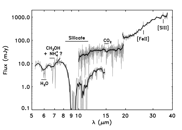
Figure 2.— SED and spectrum of B$335$. Top panel: Different symbols represent fluxes measured at the different beam sizes indicated in the legend; these data are listed in Table 2. The magnitude of possible aperture corrections in the 3 to 10 µm region can be judged by the crosses, which are photometry measured in a $1\farcs 2$ aperture (point-source). The black line shows the IRS data smoothed to $\sim\!0.4$ µm. Bottom panel: The grey line shows the IRS spectrum at full resolution; the black line shows the same data smoothed to $\sim\!0.4$ µm. Various features are indicated in the spectrum. Both panels: The IRS spectra do not join because the high resolution spectrum, from 10 to 20 µm, has a larger slit than the low resolution spectrum, from 5 to 14 µm; hence the longer wavelengths include more extended emission.

MIPS instrument observations were carried out using scan map mode in all three MIPS bands at 24 µm, 70 µm, and 160 µm as part of Spitzer program ID 53 (P.I. G. Rieke). The data reduction was carried out using the Data Analysis Tool (DAT; Gordon et al., 2005) out following the steps outlined in a paper by Stutz et al. (2007) describing a similar study of the Bok Globule CB190; please refer to that publication for details. For B$335$, the observations covered a field of $\sim\!15\arcmin\times 55\arcmin$, with an exposure time of $\sim\!192$ s at 24 µm, $\sim\!80$ s at 70 µm, and $\sim\!20$ s at 160 µm, although the integration time varies significantly in each map due to non–uniform coverage.

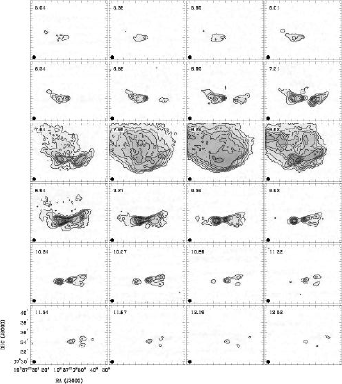
Figure 3.— Large ¹²CO J = 2 – 1 OTF channel map of B$335$, $16\arcmin\times 12\arcmin$ in size, showing channels with significant emission, from 12.52 km s^-1 to 5.04 km s^-1, at a $\sim\!0.3$ km s^-1 resolution. Channel velocities are indicated in the top left corner and the beam size ($32\arcsec$) is indicated as the filled circle in the bottom left of each panel. Contour levels are $\{1,2,3,4,5,6,8,10,12,14,16\}\times 0.5$ K-T${}_{\rm A}^{*}$.

Table 1Summary of Outflow Parameters

Dist.	Mthin	RCO	VCO	TCO	Fobs	Lobs
[pc]	[$\hbox{M}_{\odot}$]	[pc]	[km s-1]	[yr]	[$\hbox{M}_{\odot}$ km s-1 yr-1]	[$\hbox{M}_{\odot}$ cm2 s-2 yr-1]
(1)	(2)	(3)	(4)	(5)	(6)	(7)
150	0.008	0.21	4.55	4.6$\times$104	7.9$\times$10-7	1.8$\times$104
250	0.02	0.36	4.55	7.7$\times$104	1.3$\times$10-6	3.0$\times$104

Note. — Outflow parameters are calculated according to the procedure described in Cabrit & Bertout (1992) and are derived from the large ($16\arcmin\times 12\arcmin)$ ¹²CO and ¹³CO maps presented in Figures 3 and 4.

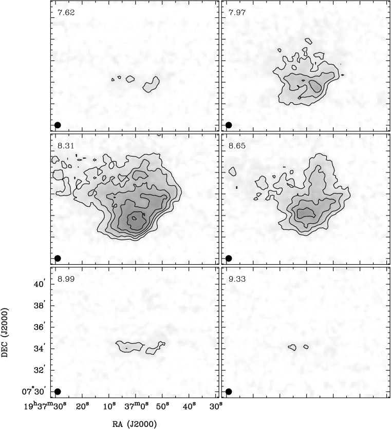
Figure 4.— Large ¹³CO J = 2 – 1 OTF channel map of B$335$, same size and spectral resolution as Figure 3. Channels with significant emission are shown, from 7.62 km s^-1 to 9.33 km s^-1. Channel velocities are indicated in the top left corner and the beam size ($32\arcsec$) is indicated as the filled circle in the bottom left of each panel. Contour levels are $\{1,2,3,4,5,6\}\times 0.5$ K-T${}_{\rm A}^{*}$.

Table 2B$335$ Photometry

$\lambda$	Beam	Flux	Error
[$\micron$]	[$\arcsec$]	[mJy]	[mJy]
(1)	(2)	(3)	(4)
3.6	2.4	0.06	0.01
“	24.0	3.16	0.30
4.5	2.4	0.49	0.05
“	24.0	12.76	1.00
5.8	2.4	0.70	0.07
“	24.0	26.06	2.50
8.0	2.4	0.72	0.07
“	24.0	21.77	2.00
24	26.0	173	16
70	70.0	15415	2090
160	40.0	28397	6167
“	90.0	67250	15250
“	100.0	68091	15231
“	360.0	160360	31090
350a	40.0	25900	4100
360b	40.0	33000	1700
360b	55.0	41000	2800
450c	40.0	14600	2200
450c	120.0	21100	3300
850c	40.0	2280	300
850c	120.0	3910	220

The IRAC data were processed by the Spitzer Science Center (SSC) using the standard data pipeline (version 11.4) to produce basic calibrated data (BCD) images. To process the BCDs and produce mosaics, we used a set of IDL procedures and csh scripts (for data handling and module control) that were provided by Sean Carey of the Spitzer instrument support team. These routines use existing MOPEX software developed by the Spitzer Science Center (Makovoz & Marleau, 2005). We produced final mosaics with a pixel scale of $0\farcs 6$ (see Figure 1). Source extraction and photometry were performed using the SExtractor software (Bertin & Arnouts, 1996). An aperture with a diameter of 8 pixels was used in the extraction. Aperture correction factors, derived by the Spitzer Science Center and provided in the IRAC Data Handbook 2.0, were used to estimate the true flux of objects based on the measured flux in each aperture. These fluxes were then converted into magnitudes using the zero magnitude flux values taken from the IRAC Data Handbook. The overall flux calibration, expressed in physical units of MJy sr^-1, is estimated by the SSC to be accurate to within 10%. All the Spitzer images are displayed in Figure 1; even at 8.0 µm the embeded point source is not visible and the images are dominated by reflection nebulosity. The Spitzer photometry is plotted in Figure 2 along with longer wavelength data taken from the literature.

IRS observations of B335 were taken in mapping mode as part of the IRS Disks GTO program 02, AOR key 3567360. The source was observed with three modules: short-hi, long-hi, and short-lo [both first and second orders]. A small raster map consisting of two positions parallel to the slit and three perpendicular to the slit was made with each module. The raster spacings parallel to the slit were selected so that the usual IRS staring mode point source measurement - which consists of measurements at positions one third of the slit length from either end - could be reconstructed from the central of the three perpendicular positions. The spacings perpendicular to the slit were a little more than half of the slit width. The observations at each raster position were carried out with an integration time of 6.3 sec.

Examination of the two dimensional spectral images shows the source to be compact along the slit. Thus, the reduction has been carried out using only the central perpendicular position from each module, as though the data were the result of an IRS staring mode observation. The position of this point source, as defined by the raster parameters, is RA = $19^{h}37^{m}0.89^{s}$, Dec = $+07^{o}34\arcmin 9.84\arcsec$ (all positions in this work are given in the J2000 system). A small amount of extended emission may have been missed in this process. The synthetic point source observations were reduced using the Cubism software (Smith et al., 2007). The spectrum is shown in Figure 2.

2.2. ¹²CO and ¹³CO data

The B$335$ region was mapped in the J=2–1 transitions of ¹²CO and ¹³CO with the 10-m diameter Heinrich Hertz Telescope (HHT) on Mt. Graham, Arizona on April 22nd, 2007. The observations were made with the 1.3mm ALMA sideband separating receiver with a 4 - 6 GHz IF band. The ¹²CO J=2-1 line at 230.538 GHz was placed in the upper sideband and the ¹³CO J=2-1 line at 220.399 GHz in the lower sideband, with a small offset in frequency to ensure that the two lines were adequately separated in the IF band. The spectrometers, one for each of the two polarizations, were filter banks with 256 channels of 250 KHz width and separation. At the observing frequencies, the spectral resolution was $\sim\!0.3$ km s^-1 and the angular resolution of the telescope was 32$\arcsec$ (FWHM). The main beam efficiency, measured from planets, was $0.85\pm 0.4$.

A $16\arcmin\times 12\arcmin$ field centered at RA = $19^{h}37^{m}00.4^{s}$, Dec = $+07^{o}35\arcmin 29\arcsec$ was mapped with on-the-fly (OTF) scanning in RA at $10\arcsec$ s^-1, with row spacing of $10\arcsec$ in declination, over a total of 72 rows. System temperatures were calibrated by the standard ambient temperature load method (Kutner & Ulich, 1981) after every other row of the map grid. Atmospheric conditions were clear and stable, and the system temperatures were nearly constant, and averaged $T_{sys}=191$ K (SSB).

Data for each CO isotopomer were processed with the CLASS reduction package (from the University of Grenoble Astrophysics Group), by removing a linear baseline and convolving the data to a square grid with $10\arcsec$ grid spacing (equal to one-third the telescope beamwidth). The intensity scales for the two polarizations were determined from observations of standard sources made just before the OTF maps. The gridded spectral data cubes were processed with the Miriad software package (Sault et al., 1995) for further analysis. This process yielded images with rms noise per pixel and per velocity channel of 0.21 K-T${}_{A}^{*}$ for both the ¹²CO and ¹³CO transitions. The ¹²CO and ¹³CO channel maps are shown in Figures 3 and 4, respectively.

Using the same set-up as that outlined above, we made a deeper map of a $2\farcm 5\times 4\farcm 5$ region centered at RA = $19^{h}37^{m}00.8^{s}$, Dec = $+07^{o}34\arcmin 07\arcsec$, near the protostar. These observations were carried out on March 19, 2008, and were repeated 7 times. The average $T_{sys}=205$ K (SSB), and was nearly constant throughout the observations. After combining the 14 images with weights proportional to the individual map rms values, we obtain final rms values per pixel and per velocity channel of $\sigma_{\rm T_{\rm A}^{*}}=0.091$ K (¹²CO) and $\sigma_{\rm T_{\rm A}^{*}}=0.084$ K (¹³CO). These maps are shown in Figures 5 and 6, while Figure 7 shows position-velocity diagrams derived from the same data.

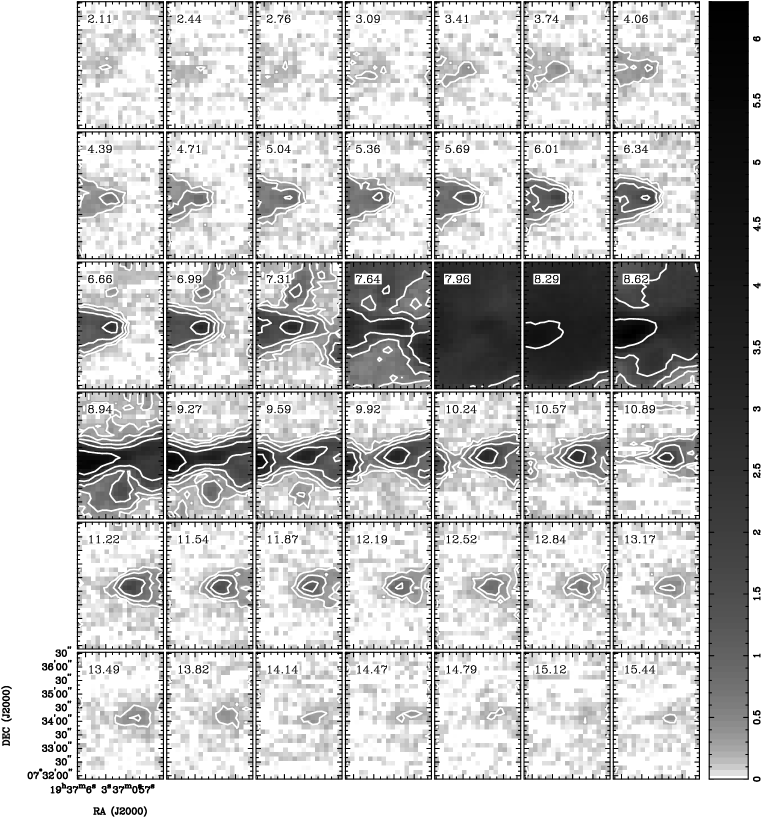
Figure 5.— ¹²CO J = 2 – 1 OTF sub-field channel map of B$335$, $2\farcm 5\times 4\farcm 5$ in size, centered on RA = $19^{h}37^{m}00.8^{s}$, Dec = $+07\arcdeg 34\arcmin 07\farcs 4$, near the location of the protostar. Channels with significant emission are shown, from 15.44 km s^-1 to 2.11 km s^-1, observed at a resolution $\sim\!0,3$ km s^-1. The temperature scale is indicated in the right side; contour levels are $\{1,2,4,8,16\}\times 0.25$ K-T${}_{\rm A}^{*}$. Note the structures located north and south of the main east-west outflow region, visible here in the south at $\sim\!9.27$ km s^-1 and in the north at $\sim\!7.31$ km s^-1.

3. The Distance

A quantitative interpretation of our observations requires an estimate of the distance to B$335$. Here we examine the often-quoted and widely accepted Tomita et al. (1979) distance to B$335$ of 250 pc and update it with modern data.

Tomita et al. (1979) derive a distance to B$335$ ranging from 130 to 250 pc, based on photoelectric stellar data from the Blanco et al. (1970) catalog, and a distance of 600 pc based on star counts. They adopt 250 pc as a plausible value but do not provide further details or show figures of $A_{V}$ vs. distance or of stellar density in the field of interest. The Blanco et al. (1970) catalog data in the region of B$335$ originates from Bouigue et al. (1961) catalog photometry. For completeness we note that the origin of the spectral types of the stars listed in the Bouigue et al. (1961) catalog are from an evidently unpublished provisional spectral classification determined by l’Observatoire de Marseille; the quoted spectral types appear generally reliable but do not always agree with those quoted in SIMBAD. The Blanco et al. (1970) catalog references 9 stars (Bouigue et al., 1961) within 45$\arcmin$ of B$335$, well outside the optical extinction extent of B$335$, $r\sim 3\arcmin$. Therefore, the Tomita et al. (1979) distance of 250 pc is highly uncertain.

We show an updated version of the $A_{B}$ vs. distance plot in Figure 8. The data are from the on-line VizieR service. We find 32 stars within $20\arcmin$ of B$335$ with spectral classifications. Of these, we reject all stars without both B-band and K-band photometry, as well as those with spectral classifications of G2 or later. Later-type stars mostly add scatter to our analysis because a small error in the spectral type yields a large error in both $A_{B}$ and distance. In all cases for which we do not have a luminosity class we assume that the star is on the main sequence. We assume $A_{B}=1.09\times E(B-K)$ (Rieke & Lebofsky, 1985). The resulting data are presented in fig. 8. We also indicate the Tomita et al. (1979) distance estimates (at 130, 250, and 600 pc) as dotted lines. We do not see any noticeable feature at or near 250 pc. To put a lower bound on the distance we use the Lallement et al. (2003) maps of the Local Bubble; in the direction of B$335$ ($l=44.9^{o},b=-6.6^{o}$) they measure the extent of the local low density bubble to be $\sim\!60$ pc. We set the upper limit to the distance to B$335$ to be $\sim\!200$ pc since in Figure 8 we see approximately constant stellar $A_{B}$ values outside of this distance. We adopt a distance of 150 pc in the following discussion, indicated as a solid line in Figure 8. Our adopted distance is uncertain by nearly a factor of two, but it falls near the middle of the plausible range. It also reduces a number of discrepancies found by Harvey et al. (2001) in modeling the extinction of the globule, and helps reconcile the inferred properties for the protostar with the luminosity of the globule (see § 5).

4. Resolved Structure

4.1. The Outflow

The ¹²CO and ¹³CO maps are presented in Figures 3 through 7. The large maps ($16\arcmin\times 12\arcmin$) show the full spatial extent ($\sim\!8\arcmin$) of the outflow as well as the velocity extent. The western side of the outflow is redshifted with respect to the line of sight while the eastern side is blueshifted. These maps are also used by Shirley et al. (2008, in preparation) to calculate the outflow opening angle. They use this angle ($\sim\!55\arcdeg$) to exclude from their analysis of the submillimeter dust opacities regions where dust may be affected by processes such as shock heating. The ¹²CO and ¹³CO lines are well resolved with 250 KHz ($\sim\!0.3$ km s^-1) channel width; in ¹²CO the blueshifted lobe is dominated by velocities ranging from $\sim\!5.04$ to $\sim\!6.99$ km s^-1 while the redshifted velocities range from $\sim\!9.27$ to $\sim\!12.52$ km s^-1 (see Figure 3). The subfield map (Fig. 5) shows that the velocity extent of the red- and blueshifted emission is in fact larger; however, these maps do not cover the full $8\arcmin$ region of the outflow. The ¹³CO data do not show an outflow; the range of these velocities is much narrower than the ¹²CO velocities, from about 9.33 to 7.62 km s^-1. The ¹³CO data are dominated by colder emission: in the large map (Fig. 4) we see little evidence of the outflow lobes observed in ¹²CO. However, some east-west elongation can be observed in the sub-field map, see Figure 6, due to the lower noise (rms $\sim\!0.084$ K-T${}_{A}^{*}$) in the smaller map as compared to the full field map (rms $\sim\!0.21$ K-T${}_{A}^{*}$). Both large maps show an extension of emission to the north and east of the protostar, on a scale of $\sim\!9\arcmin$ in ¹²CO and $\sim\!6\arcmin$ in ¹³CO, which is also observed in the 160 µm mosaic. The outflow parameters calculated from the large area maps are presented in Table 1.

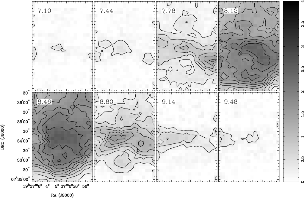
Figure 6.— ¹³CO J = 2 – 1 map; same as Figure 5. Channels with significant emission are shown, from 7.10 km s^-1 to 9.48 km s^-1. Contour levels are $\{1,2,3,4,5,6,7,8,9\}\times 0.25$ K-T${}_{\rm A}^{*}$.

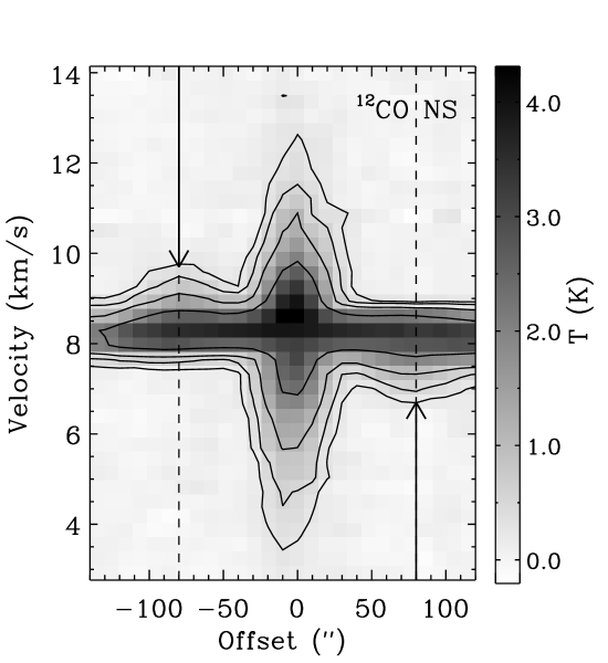
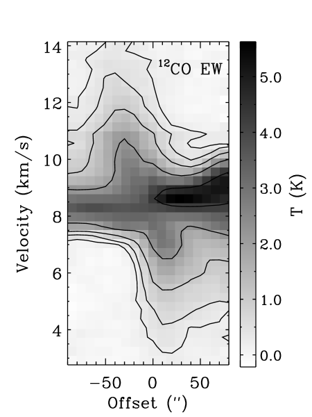
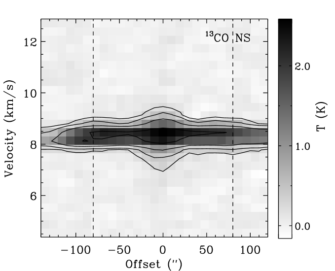
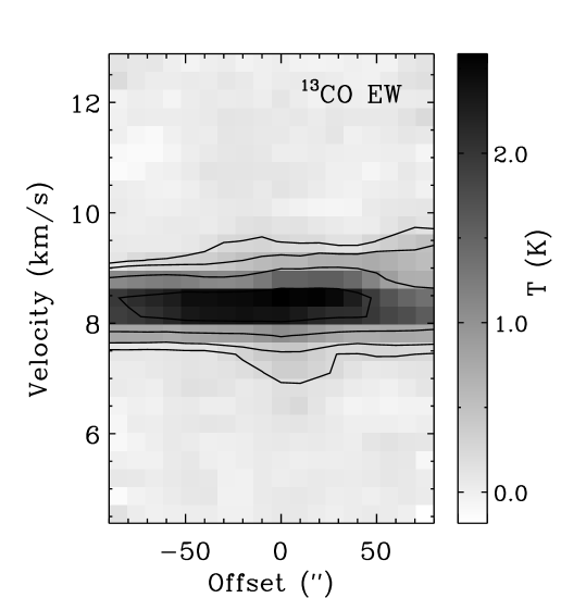
Figure 7.— ¹²CO (top) and ¹³CO (bottom) position-velocity diagrams for the sub–field map. The ¹²CO contour levels are $\{1,2,4,8,16\}\times 3\sigma$, where $3\sigma=$0.28 K-T${}_{\rm A}^{*}$. The ¹³CO contour levels are also $\{1,2,4,8\}\times 3\sigma$, where $3\sigma=0.25$ K-T${}_{\rm A}^{*}$. The ¹²CO north-south cut is centered on RA = $19^{h}37^{m}0.75^{s}$; the east-west cut is centered on Dec = $07^{o}34\arcmin 7\farcs 05$. The ¹³CO north-south cut is centered on RA = $19^{h}37^{m}0.83^{s}$; the east-west cut is centered on Dec = $07^{o}34\arcmin 5\farcs 26$. The vertical lines (dashed and solid arrows) in the ¹²CO and ¹³CO NS cuts indicate the offsets ($80\arcsec$) at which the flattened molecular core is detected.

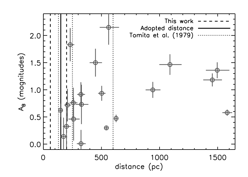
Figure 8.— $A_{B}$ vs. distance for stars within 20$\arcmin$ of B$335$. The error bars indicate the magnitude of the effect of a 15% change in each direction in the $(B-K)$ color. The dotted lines indicate the range in distances derived by Tomita et al. (1979): 130, 250 (adopted by those authors), and 600 pc, respectively. Note that we do not reproduce a discontinuity in $A_{B}$ at 250 pc. The dashed lines indicate plausible ranges in the distance based on the measured extent of the local bubble and the $A_{B}$ data shown here (see § 3): 60 and 200 pc. Our adopted distance of 150 pc is indicated by the solid line, and represents a conservative estimate.

The IRAC images reveal a resolved emission structure consisting of two outflow lobes oriented in the east-west direction, seen clearly in Figure 1 in all four IRAC channels. The observation that the eastern lobe is brighter than its western counterpart is explained by the fact that the outflow is oriented slightly out of the plane of sky; this orientation is corroborated by our CO maps in which the eastern lobe is slightly blueshifted relative to the western lobe, as discussed above. It is also in agreement with other measurements: for example, Cabrit & Bertout (1992) measured the inclination angle to the line of sight to be $82\arcdeg$. The outflow not being aligned exactly on the plane of the sky will give rise to differential extinction between the eastern and western lobes, causing the western lobe to be more obscured by the surrounding cold globule material out of which the protostar was formed.

To improve the spatial resolution of the Spitzer data, we present the deconvolved HiRes images of B$335$ in Figure 9 (right-hand column). We reprocessed the raw (BCD) data from the Spitzer archive, using a version of HiRes deconvolution developed for Spitzer images by Backus et al. (2005) based on the Richardson-Lucy algorithm (Richardson, 1972; Lucy, 1974) and the Maximum Correlation Method (Aumann et al., 1990). HiRes deconvolution improves the visualization of spatial morphology by enhancing resolution (to sub-arcsec levels in the IRAC bands) and removing the contaminating sidelobes from bright sources (Velusamy et al., 2008). It achieves a factor of 3 enhancement over the diffraction limited spatial resolution from $\sim$ 1.22$\lambda$/D to $\sim$ 0.4 $\lambda$/D (e.g. from 2.4″to $\sim$ 0.8″at 8$\mu$m). Typically the diffraction residue in the HiRes images is at levels well below 0.1% to 1% for the IRAC and MIPS 24 µm bands. The Point-source Response Functions (PRFs), required as inputs to HiRes, were obtained from the SSC; we used the extended (about 128 detector pixel size in each direction) versions, supplied by Tom Jarrett (private communication, 2007). The observed images, in the form of raw BCDs, were first post processed to fix contaminated data for saturation, column pulldown, muxbleed, muxstriping, jailbars, and outliers. In the Richardson-Lucy algorithm the best resolution enhancement is attained when the background is zero. Accordingly, we used the background subtracted BCDs. In HiRes we used 50 iterations for the IRAC bands and 100 for MIPS, which resulted in a FWHM of 0.55″to 0.75″for IRAC channels 1-4 and 1.6″at 24 µm for a point source in the deconvolved images. All bands are relatively clean from artifacts except IRAC channel 4 (at 8$\mu$m) which has some uncorrected muxbleed. In the HiRes images diffraction residues near the Airy rings are low (at a level $<$ 0.05% of the respective peak intensities at 3.6, 4.5, and 5.8 $\mu$m) providing enhanced visualization closer to the protostar.

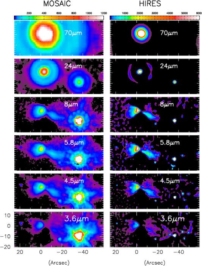
Figure 9.— Gallery of images of B335 (CB199) at the indicated wavelengths. The images in the right column have been processed with HiRes for improved spatial resolution. North is up and east is to the left.

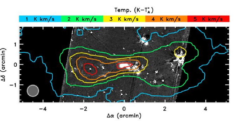
Figure 10.— IRAC 4.5 µm minus 3.5 µm image with ¹²CO integrated contours at the indicated temperatures. The countours are integrated over 0 to 15 km s^-1. The beam size ($32\arcsec$) is indicated by the grey circle. Note the presence of HH objects, knots of dense shocked material producing molecular-H emission, located near the southern and eastern regions of the 4 K km/s contour. North is up and east is to the left.

In the HiRes 5.8 µm image we measure the outflow opening angle to be about $70\arcdeg$, while in the deconvolved 8.0 µm image we measure the angle to be between $62\arcdeg$ and $67\arcdeg$. Shirley et al. 2008 (in preparation) measure the ¹²CO outflow opening angle to be closer to $55\arcdeg$. In Figure 10 we show the ¹²CO integrated contours overlaid on the IRAC 4.5 µm minus 3.6 µm image. It appears that the molecular outflow is more confined than if it were simply expanding from the opening angle inferred from the IRAC images. Also note the presence of Herbig Haro (HH) objects in the subtracted image along the inner walls of the confining cavity, where it is probable that dense shocked gas produces molecular hydrogen and CO emission that accounts for much of the signal in the IRAC images. These emission features fall in IRAC channel 2. The HH objects (some having a striking filamentary geometry) imply that the inner cavity wall is quite sharp. More detailed discussion of the B$335$ HH objects can be found in, e.g., Gâlfalk & Olofsson (2007) and Galván-Madrid et al. (2004).

The IRS spectrum (see Figure 2) shows emission lines at $\sim\!26$ µm and $\sim\!35$ µm which we identify as [FeII] and [SiII], respectively. These lines may be produced in the interaction between the outflow and the surrounding neutral material. We note that they are also seen in the spectrum of the north-east lobe (HH47A) in the HH46/47 outflow, as discussed by Noriega-Crespo et al. (2004) and Velusamy et al. (2007). We also observe other features of interest in the IRS spectrum, indicated in Figure 2, like H₂O and CO₂ ices and a deep silicate absorption feature (van Dishoeck, 2004).

4.2. The Shadow

The IRAC images show a shadow, located near the outflow lobes. In Figure 1 the shadow is evident at 3.6 µm and 8.0 µm, just to the south of the outflow lobes, as a dark nearly circular feature about $20\arcsec$ in extent. We also marginally detect a northern counterpart in the 3.6 µm and 8.0 µm images (see Figures 1 and 11). We show the IRAC images on a log scale, with the minimum and maximum image values set to highlight the shadow and the outflow lobes; no other special processing of the images was used to display the images.

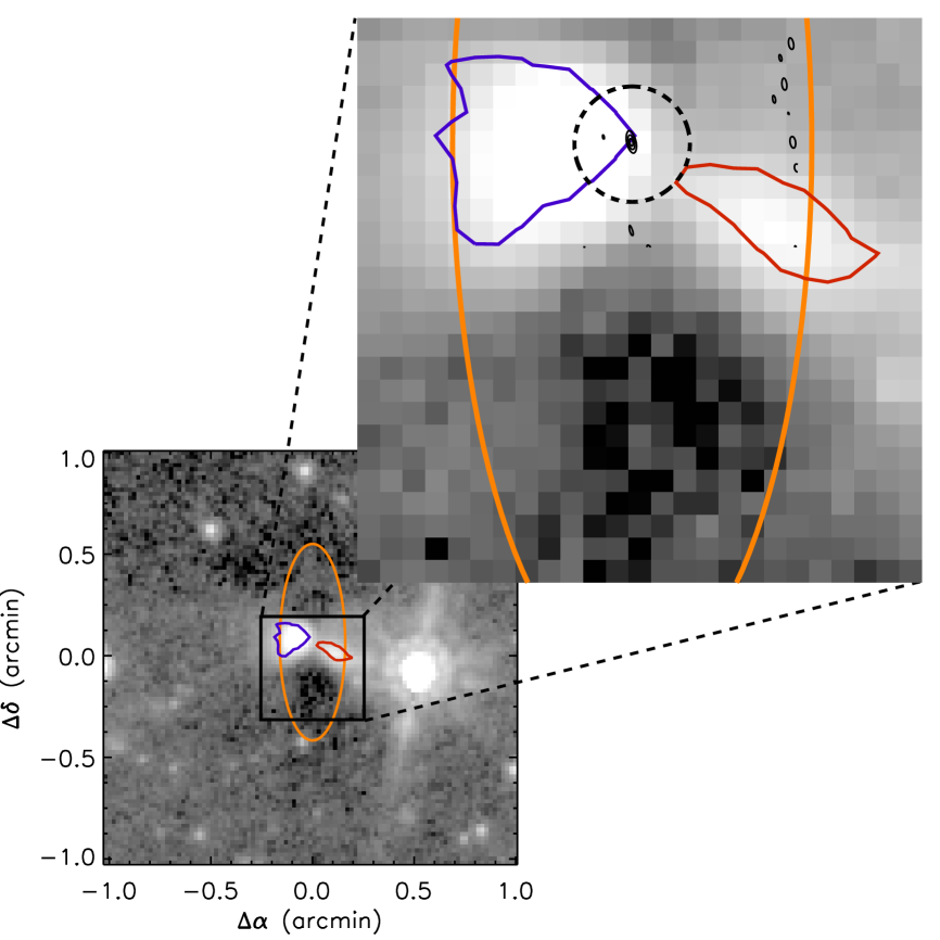
Figure 11.— IRAC 8.0 µm image of B$335$, with inset, both shown on a log scale and at the original mosaic pixel scale of $1\farcs 2$ pix^-1. The 8.0 µm shadow can be observed near the center and just south of the protostar. We also show the HiRes 8.0 µm deconvolved contours in red (west) and blue (east); these colors correspond to the CO outflow kinematics. The orange ellipse has a 3:1 major to minor aspect ratio and indicates the rough size and shape of the flattened molecular core. Inset: The solid black contours indicate the location of the circumstellar disk ($\sim$ 200 AU) observed at 1.2 mm by Harvey et al. (2003a); the black dashed circle (with 3$\arcsec$ radius) indicates the 24 µm PSF. North is up and east is to the left.

The likely cause of the IRAC shadow is dense globule (dust and molecular) material near the protostar. The observed difference in brightness between the east and west outflow lobes (apparent at all IRAC wavelengths, see Figures 1 and 9), is explained by: (a) the outflow orientation with the eastern lobe pointing slightly towards the observer, and (b) the presence of dense material at large radii (compared to the $\sim\!200$ AU circumstellar disk) causing differential extinction between the two lobes. This interpretation is supported by the spatial distribution and measured color excesses observed by Harvey et al. (2001). These data are presented in Figure 12, where we show the locations of the stellar sources (circles) overlaid on the binned 8.0 µm image. Here the colors indicate a rough extinction distribution for the Harvey et al. (2001) sources: red circles indicate sources with $(H-K)$ color excess greater that 2.9 (equal to the mean value plus $2\times$ the rms in the color excess distribution), the orange circles indicate color excesses between 2.1 (equal to the mean value plus $1\times$ the rms in the color excess distribution) and 2.9, and the yellow circles indicate sources with excesses less than 2.1. In this figure, the ellipse (with a 3:2 major to minor axis ratio) indicates the rough shape of the hole devoid of stars near the center of the cloud. The location of the most obscured sources around the outer circumference of the southern shadow is suggestive that the shadow is in fact tracing a flattened overdensity in molecular material. On the northern side the shadow is also detected in the IRAC image; its location, like the southern counterpart, is bounded by background stellar detections, indicating that the molecular core is in fact flattened and that it has a significant degree of symmetry.

In the text that follows we analyze the shadow and derive optical depth and density profiles; we use techniques similar to those presented in Stutz et al. (2007). The shadow is roughly centered on RA = $19^{h}37^{m}01^{s}$, Dec = $+07^{o}33\arcmin 55\arcsec$. Although the shadow is observed at both 3.6 µm and 8.0 µm we apply the following analysis only to the 8.0 µm shadow because the 3.6 µm image has too many complicating factors, namely contamination from the nearby bright source just west of B$335$ and many more stellar sources in and around the region of interest. In summary, to derive an 8.0 µm profile we go through the following steps: (1) re-normalize the image to our best estimate of the true background value (Figure 13), (2) divide the image up into regions inside and outside of the shadow (Figure 14), (3) use these regions to derive optical depth, density, and extinction profiles, all of which are equivalent, the latter two being subject to an assumption about the dust properties at the wavelength of interest (Figure 15), and (4), compare the derived profile to available stellar color excesses, in this case the Harvey et al. (2001) data, see Figure 16. Here we discuss this process in more detail.

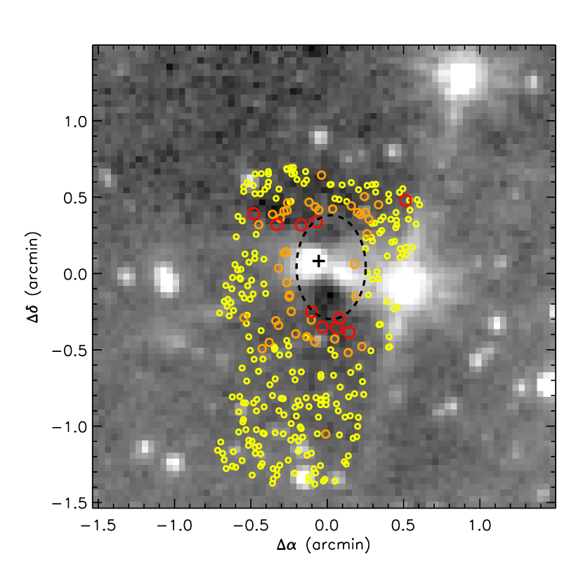
Figure 12.— IRAC 8.0 µm image of B$335$, binned 2$\times$2 for a $2\farcs 4$ pix^-1 resolution. The 8.0 µm shadow can be observed near the center and just south of the outflow lobes; a northern shadow counterpart is marginally dectected. The circles indicate the locations of Harvey et al. (2001) near-IR stellar sources: the large red circles indicate sources with $(H-K)$ color excesses greater than 2.9 (2$\sigma$, where for this set of observations $\sigma=0.8$), the medium orange circles indicate sources with color excesses between 2.1 (1$\sigma$) and 2.9, and the small yellow circles indicate sources with excesses below 2.1. The cross indicates the location of the Harvey et al. (2003a) detection of the central source. The dashed ellipse (shown with a 3:2 axis ratio) is meant to highlight the shape of the inner region without stellar detections. North is up and east is to the left.

The background level in the images, which we term $f_{DC}$ and which is composed of instrumental background and zodiacal background, must be measured and subtracted from the images to analyze the shadow. We estimate $f_{DC}$ by adjusting the level so that the depth of the shadow and the extinction inferred from stellar observations agree. We compare this level with the pixel values in a $2\farcm 2$ squared box located $2\farcm 2$ north of the source selected for minimum surface brightness; the distribution of pixel values is shown in Figure 13. The chosen value for $f_{DC}=827.40$ MJy sr^-1 is the 6th percentile pixel value in the box. The reasonably good agreement between our detected background and the assumed one validates our procedure.

Figure 13.— IRAC 8.0 µm pixel value distribution for a region $2\farcm 2$ on a side, $2\farcm 2$ north of B335. The solid line indicates the 6th percentile value that we use for the image background value, equal to 827.408 MJy sr^-1, chosen to get the best match to the stellar extinction values from Harvey et al. (2001).

Figure 14.— IRAC 8.0 µm image of B335, with two stars masked out (black boxes). The blue ellipses, centered on the Harvey et al. location for the protostar (marked with a green circle) indicate the nested and adjacent regions we define to analyze the shadow. The green lines indicate a $60\arcdeg$ wedge between position angles 240$\arcdeg$ and 300$\arcdeg$, outside of which we reject all pixels due to light contamination from (a) the protostar reflection lobes, and (b) the diffraction spikes from the nearby very bright source.

Figure 15.— IRAC 8.0µm shadow profile. Top panel: Average pixel values as a function of major axis distance from the Harvey et al. (2003a) location of the protostar. Solid, short-dashed, and dotted lines indicate, respectively, the derived unobscured flux levels ($I_{0}$) in the three indicated regions: the full 60$\arcdeg$ wedge, the eastern 30$\arcdeg$ half, and the western 30$\arcdeg$ half (located at the position angles indicated in teh top panel). The vertical long-dashed line indicates the six outer regions used to derive $I_{0}$. Bottom panel: $\exp(-\tau)=I/I_{0}$ as a function of major axis distance from the Harvey et al. (2003a) location of the protostar. Both panels: Squares indicate the profile derived using the full 60$\arcdeg$ wedge, triangles indicate the eastern 30$\arcdeg$ half of the wedge, and crosses indicate the western 30$\arcdeg$ half of the wedge. The bounding position angles of these wedges (240$\arcdeg$, 270$\arcdeg$, and 300$\arcdeg$) are indicated in the top panel. Note that there are not significant differences between the profiles, indicating that the derived profile is not strongly affected by the nearby bright source.

We divide the image into nested and concentric elliptical regions shown in Figure 14. The elliptical regions are centered on the Harvey et al. (2003a) location of the protostar, and have a major-to-minor axis ratio of 3:1. The ratio was chosen to match roughly the location and shape of the 8.0 µm shadow and to satisfy the mininum requirements of the observed geometry: inspection of Figure 14 provides the constraint that the flattened core must lie in front of the entire western outflow lobe while still providing the obscuration observed as a shadow at 8.0 µm. Smaller axis ratios (rounder ellipses) will violate these constraints. Similarly, larger axis ratios may allow for some of the emission from the outer region of the western lobe to appear unobscured. We reject all pixels outside of a 60$\arcdeg$ wide wedge pointed directly south; this wedge is indicated as two green lines in Figure 14. It was chosen to avoid the diffraction spikes of the nearby bright star and to mask out regions affected by emission from the outflow lobes. As can be seen in Figure 14, we also mask out two bright sources (black boxes) that would have affected the shadow profile. We then tabulate the mean pixel value in each elliptical region, plotted in Figure 15 (upper panel, square symbols). We use this distribution to calculate an estimate of the optical depth, $\tau=-\ln(I/I_{0})$, in the shadow. To do so we must measure $I_{0}$, the unobscured flux level near the shadow. We measure $I_{0}$ from the regions where the mean pixel values approach a constant, in this case at elliptical major axis values greater than 56$\arcsec$. We average over all pixel values outside this region and inside 78$\arcsec$; we measure the value of $I_{0}=8.26$, indicated in the upper panel of Figure 15 as a solid line. In the lower panel of Figure 15 we plot $\exp(-\tau_{8})=I/I_{0}$ versus major axis distance. One can clearly see that the inner-most region is greatly affected by emission from the outflow lobes.

Motivated by the concern that emission from the bright source just to the west of B$335$ could be affecting our derived shadow profile we perform the following test. We divide the 60$\arcdeg$ wedge between position angles 240$\arcdeg$ and 300$\arcdeg$ into two 30$\arcdeg$ wedges, one on the east side, away from the bright source, and one on the west side. We proceed with the same analysis as described above and plot the resulting profiles in Figure 15. These profiles (triangles indicate the east wedge, crosses indicate the west wedge) do not show significant variations between each other, or relative to the full wedge (again, indicated as squares). Therefore the nearby bright source is not significantly affecting our shadow profile.

Finally, using this $\tau$-profile, we derive an extinction profile. Following the convention outlined in Stutz et al. (2007), and assuming an 8.0 µm dust opacity of $\kappa_{abs,8}=8.13\times 10^{2}$ cm² gm^-1 calculated by Draine (2003a, b) from his $R_{V}=5.5$ model, we derive the $A_{V}$ profile plotted in Figure 16. Here, the average mass column density in each elliptical annulus is given by

$$\Sigma=\frac{\tau_{8}}{\kappa_{abs,8}}f,$$ (1)

where $f(=100)$ is the gas-to-dust ratio, and $\kappa_{abs,8}$ is the absorption cross-section per mass of dust, and has the assumed value noted above. The choice of a model with a high $R_{V}$ value relative to the diffuse ISM is intended to account for the grain coagulation expected in dense, cold cores. The extinction profile is given by

$$A_{V}=\frac{\Sigma}{1.87\times 10^{21}\,{\rm cm}^{-2}\,{\rm mag}^{-1}\mu_{\rm H_{2}}m_{\rm H}}.$$ (2)

We have assumed the conversion factor from the relation $N(H_{2})/A_{V}=1.87\times 10^{21}$ atoms cm^-2 mag^-1 (Bohlin et al., 1978), where we assume that all of the hydrogen is in molecular form. We have adopted $R_{V}=3.1$ — a value appropriate for the diffuse ISM where this relation was measured — to convert the Bohlin et al. (1978) relation from $E(B-V)$ to $A_{V}$. At longer wavelengths than $V$ the extinction law does not appear to be a strong function of density. Here $\mu_{\rm H_{2}}=2.8$ is the effective molecular weight per hydrogen molecule. For this set of constants $A_{V}=14.04\times\tau_{8}$. Following a different method, where the conversion is obtained directly from the Draine (2003a, b) dust models, $A_{V}=\kappa_{abs,V}/\kappa_{abs,8}\times A_{8}=9.7\times\tau_{8}$. The two $A_{V}$ determinations are consistent within the uncertainties of the measured infrared extinction values (see below). To take possible freezeout and grain growth effects into account we consider the Ossenkopf & Henning (1994) model opacities; for models generated at a density of $n=10^{6}$ cm^-3 these authors derive 8.0 µm opacities of $\kappa_{abs,8}=1.06\times 10^{3}$ cm² gm^-1 and $\kappa_{abs,8}=1.21\times 10^{3}$ cm² gm^-1 for thin and thick grains, respectively. These opacities will diminish the derived $A_{V}$ values by factors of 1.3 and 1.5 respectively. We note that the range in measured infrared extinction (e.g., Indebetouw et al., 2005; Flaherty et al., 2007) is significant; the $A_{V}$ determination is therefore uncertain by a factor $\sim\!2$ and as a result so is the column density.

Figure 16 shows the derived shadow extinction profile (square symbols); we compare our profile to the values derived from the Harvey et al. (2001) stellar data in each elliptical region. To make use of the stellar observed $(H-K)$ colors we follow the procedure in Harvey et al. (2001). In addition to the statistical uncertainty in $(H-K)$, they also measured the uncertainty due to the intrinsic scatter in $(H-K)$ of background stars determined from a nearby “OFF” field. The mean intrinsic $(H-K)=0.13\pm 0.16$ for the “OFF” field. To determine the color excess, the stellar $(H-K)$ colors have 0.13 subtracted from them; to determine the total errors we add $0.16$ in quadrature to the statistical errors. Finally, we use $A_{V}/E(H-K)=15.87$ to convert to $A_{V}$ (Rieke & Lebofsky, 1985). To make a fair comparison between the shadow profile and the stellar color exess, we must subtract off the mean value of the stellar extinction in the regions used to find $I_{0}$ for the shadow, i.e. we account for the differences in the two zero-points for the profiles. In this case, $\langle A_{V}\rangle=14.52$, or $E(H-K)=0.92$, for the stars in this region.

The maximum extinction level derived for the shadow is $A_{V}\sim 100$. Our spectrum (Fig. 2) shows silicate absorption with a $\tau\gtrsim 2.5$. Because of possible complexities with interpreting this spectrum, we consider $\tau\sim 2.5$. Applying a standard conversion (Rieke & Lebofsky, 1985) the corresponding extinction is $A_{V}\gtrsim 40$. We interpret the measurement as a lower limit because radiative transfer in a disk with a temperature gradient will tend to fill in the intrinsic feature. If we assume an equal amount of material behind the star, the limit on the total column is equivalent to $A_{V}\gtrsim 80$. Thus, the spectrum is consistent with our shadow analysis: there is a column density of N(H₂)$\sim 10^{23}$ cm^-2 or more towards the protostar. For a radius of $20\arcsec$, this column yields a mass $\sim\!0.5$ $\hbox{M}_{\odot}$.

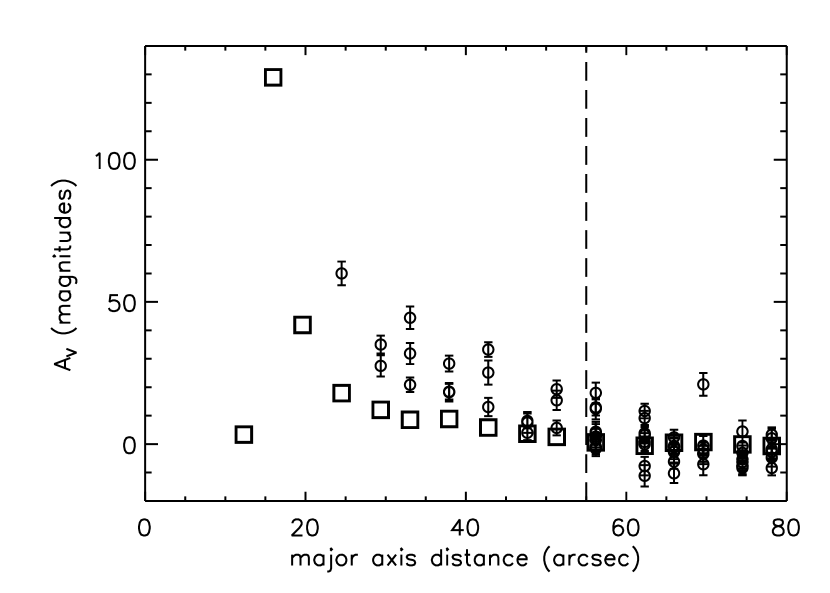
Figure 16.— $A_{V}$ values for the 8.0 µm shadow (squares) compared to the Harvey et al. (2001) stellar $A_{V}$ values (circles) for each elliptical region. We use the six outer radii — indicated by the dashed line — to normalize both the shadow and stellar extinction profiles.

Figure 11 shows additional components of the source in relation to the shadow. Harvey et al. (2003a) used the IRAM interferometer in the A configuration, which has baselines of 43 to 400 m. At this high resolution they detect the protoplanetary disk in emission, with a maximum diameter of about $1\arcsec$ (150 AU, see Fig. 11), but resolve out larger structures. Harvey et al. (2003b) used the D configuration with baselines of 15 to 80 m, which allow for larger structures to be resolved. Their best fit model to the data (p = 1.65, $\alpha$ = 40$\arcdeg$, see their Figure 3) shows a structure about $7\arcsec$ in extent aligned in the north-south direction (not shown in Fig. 11). This emission likely originates from the innermost material associated with the 8.0 µm shadow. The dashed circle indicates the 24 µm PSF ($\sim\!3\arcsec$ in radius) which is coincident with the protostar and disk.

Our analysis does not include any treatment of the possible foreground emission that may arise from the surface of the globule its self; this emission, if present, would have the net effect of causing an underestimate of the derived optical depth. A rigorous modeling of this emission component is beyond the scope of this paper. However, inspection of Figure 16 indicates that if this effect is present it is not large; the Harvey et al. (2001) stellar data lie preferentially above our shadow profile, at higher $A_{V}$’s. Foreground emission could explain this systematic offset. However, other uncertainties, discussed above, are likely to dominate our extinction profile estimate.

4.3. Detection of a flattened molecular core

The sub-field ¹²CO and ¹³CO channel maps show a north-south structure that appears to be rotating, seen in Figures 5 and 6. This structure extends out to a radius of about 80$\arcsec$ (12000 AU) from the protostar. In Figure 5 the southern component is detected between roughly 8.94 km s^-1 and 9.92 km s^-1; at 8.94 km s^-1 the image is dominated by the center velocity emission. The northern counterpart is weaker in emission, but is apparent at 7.31 km s^-1 and fades at velocities smaller than 6.66 km s^-1. The maximum relative velocity between the two sides is therefore about 3 km s^-1. The ¹³CO map shows little indication of this velocity gradient; however, there is a north-south elongation of the emitting region. Additionally, CO freeze-out may complicate the analysis of the molecular data. The difference in appearance in ¹²CO between the northern and southern regions can be explained by clumpy material in a rotating structure, expected by models (see below). Thus, both our extinction shadow image and our CO line mapping indicate that the dense core of the globule is flattened and may be rotating around the protostar.

There have been many indications of this flattened structure previously, on different angular scales depending on the type of observation. For example, the 800 µm image by Chandler et al. (1990) indicates a low surface brightness north-south extension of about 2$\arcmin$, compared with only about 1$\arcmin$ for the east-west extension. Velusamy et al. (1995) find a very similar structure in their filled aperture image in CCS at 22 GHz. They also present channel maps that show no convincing evidence of overall rotation. Hodapp (1998) shows deep images at H and K that reveal shadows of the cloud against the diffuse light from the background, a technique analogous to ours at 8.0 µm. At H, the shadow is slightly flattened, but it is significantly more so at K-band. This change is probably due to the ability of the K-band image to penetrate larger optical depths than at H-band. Saito et al. (1999) show a similar structure in C¹⁸O and find marginal evidence that it is rotating with a small redshift to the north and blue shift to the south. The indicated rotation is only about 0.05 km/sec over the range of 2$\arcmin$ (0.09pc).

Wilner et al. (2000) observed in CS J = 5-4 with the IRAM interferometer and an angular resolution of 2.5$\arcsec$; their channel maps do not appear to show the full structure, but there is a signal near the systemic velocity that is well resolved with a length of $5\arcsec$ to $6\arcsec$ oriented approximately N-S. This structure is also seen in the IRAM interferometer continuum data obtained at 1.2mm simultaneously (Harvey et al., 2003b) and by Jørgensen et al. (2007) with the SMA (the latter image also shows a faint extension to the north and another to the SSW). It is plausible that the latter three references underestimate the extent of the larger, low surface bright structure because it is partially resolved out with the interferometers. This possibility is partially supported by the strong detection of the north-south structure over a length scale of $2\arcmin$ in the filled aperture CS observation by Velusamy et al. (1995).

Three-dimensional numerical simulations of cloud collapse are growing rapidly in sophistication. In general, they show that the collapse proceeds quickly into filaments, or disks with spiral arms, and with typical dimensions of 1000 AU (diameter) (Whitehouse & Bate, 2006; Krumholz et al., 2007; Arreaga-García et al., 2007), a result that was also anticipated in some earlier work (e.g., Nelson & Langer, 1997). In the simulations, these structures often break up into binary or multiple forming stellar systems with dense and more compact circumstellar/protoplanetary disks. In any case, the interstellar medium becomes organized into two distinct classes of structure: 1.) an evolving, pseudo-stable protoplanetary disk of size up to a couple of hundred AU; and 2.) what we term a flattened molecular core to include the variety of filaments, disks, and spiral arms produced by the simulations, and of typical size 1000 AU. Viewed edge-on, most versions of flattened molecular cores would appear as linear structures similar to edge-on disks. By an age of order 100,000 years or less, the natal cloud dissipates to reveal the new protostar, and the flattened molecular cores have disappeared. The protostellar disk remains, within a typical 200 AU diameter (see Andrews & Williams, 2007). In turn, it evolves and dissipates on a time scale of a few million years, leaving a planetary system with typical dimensions of 200 AU.

The B$335$ structure would appear to be similar to the elongated shadow in the IRAC images of L 1157 discovered by Looney et al. (2007). However, the L 1157 shadow is $\sim$ 15,000 to 30,000 AU in diameter, somewhat larger than that around B$335$. Looney et al. (2007) suggest that it represents a flattened density enhancement produced as a result of the general influence of magnetic fields or rotation in the collapse of a cloud; that is, it is part of the general trend that yields a flattened molecular core, but probably on a size scale that decouples much of its volume from direct participation in the formation of the central protostar.

Table 3Mass Estimates

Data	Temp.	Radius	Mass [$\hbox{M}_{\odot}$]
	[K]	[$\arcsec$]	[$\hbox{M}_{\odot}$]
(1)	(2)	(3)	(4)
8.0 $\micron$	$\cdots$	20	0.5
160 $\micron$	10	48	43
160 $\micron$	10	80	69
160 $\micron$	12	48	10
160 $\micron$	12	80	15
160 $\micron$	14	48	3.2
160 $\micron$	14	80	5.2
13CO	30	300	$\geqslant$0.08a
13CO	10	300	$\geqslant$0.2a
12COb	$\cdots$	80	35

4.4. Globule Mass

A number of lines of evidence suggest that the full globule has substantial mass. We find $\sim$ 0.5 M_⊙ within a $40\arcsec$ beam, based on the absorbing column of material. Gee et al. (1985) modeled the spectral energy distribution (fitting it with a 14 K temperature and a $\nu^{2}$ emissivity) to find a mass that translates to $\sim$ 4 $\hbox{M}_{\odot}$ at our preferred distance of 150 pc. Similar masses were derived by Keene et al. (1983) and Davidson (1987), while somewhat smaller values (by factors of $\sim$ 3) have been derived by Walker et al. (1990) and Shirley et al. (2002). Correcting these measurements to a scale comparable to the ¹²CO source diameter (e.g., according to the relative flux density versus aperture at 160$\mu$m) increases them by a factor of 2 to 3.

At the same time, the calculations depend critically on the assumed temperature of the dust. An upper limit of $\sim$ 14K can be adopted on the basis of the SED (Gee et al., 1985), plus expectations for dust temperatures due to heating by the ISRF (de Luca et al., 1993). In Table 3, we show the dependence of calculated mass on dust temperature within this constraint, both for a 40” aperture and for the full source. We conclude that the mass of the entire globule is likely to be greater than 5 $\hbox{M}_{\odot}$, perhaps even by a factor of a few.

A total cloud mass of 10 $\hbox{M}_{\odot}$, if rotationally supported against collapse, would have a net velocity gradient of $\sim\!1.5$ km s^-1. Different molecular lines give differing measures of the velocity gradient in the cloud, from zero to $\sim\!3$ km s^-1 (the latter from our ¹²CO data). From these discrepancies it is likely that the cloud is not simply in smooth rotation but probably has a complex structure in terms of both density and dynamics (e.g. Zhou et al., 1990). Nonetheless, the overall gradient we observe in ¹²CO supports the argument for a mass of $\sim\!10$ $\hbox{M}_{\odot}$ or more.

5. The Protostar

Figure 1 shows our three MIPS B$335$ mosaics. Figure 9 shows the deconvolved HiRes 24 and 70 µm images. In Figure 11 we indicate the location of the protostar from Harvey et al. (2003a) with black contours (RA = $19^{h}37^{m}0.89^{s}$, Dec = $+07^{o}34\arcmin 10.9\arcsec$). The dashed circle indicates the 24 µm PSF size, which is well centered on the radio continuum measurement. The 70 µm PSF is well centered on the protostar, while the 160 µm point-source is slightly offset most likely due to artifacts in the mosaic. The SCUBA 450 and 850 µm observations of B$335$ (Shirley et al., 2000) are also well centered on the radio observations. This object thus coincides with a bright point source seen in each of the MIPS bands. As illustrated by Figure 11, the protostar is invisible in IRAC channel 4 (and all other IRAC channels). However, in the MIPS bands it dominates the emission. We detect a small asymmetry in the 24 µm PSF in the east-west direction. This asymmetry becomes more evident in the HiRes deconvolved images. The elongation is clearly seen along the east-west direction after a PSF subtraction to take out the bright symmetric core of the PSF. We note that the direction of the 24 µm PSF asymetry (PA = $\sim\!100\arcdeg$) is somewhat misaligned with the IRAC emission (see Fig. 9) but in agreement with the ¹²CO outflow orientation (see Fig. 10). The protostar accounts for almost all of the 70 µm radiation and for the point source seen at 160 µm as well. As noted previously, the 160 µm emission is also extended to the north-west of the YSO. This extension is in the direction of the main body of globule, and can be seen in our ¹²CO and ¹³CO maps (see Figures 3 and 4).

By combining the measurements across the Spitzer bands with those at longer wavelengths from the Kuiper Airborne Observatory (KAO) and ground-based telescopes, we have produced the composite spectral energy distribution for B335 shown in Figure 2. The Spitzer images show that the infrared emission from B$335$ is confined spatially out to 70 µm. At 160 µm, the images show a compact source plus a diffuse component; these results are consistent with those of Keene (1983) showing that the flux from the source starts increasing with measurement aperture only longward of 140 µm.

In Table 2 we list the present photometric results as well as selected results taken from the literature. IRAC data are tabulated at both $2\farcs 4$ and $24\arcsec$ aperture diameters to facilitate the model comparison discussed below. At 160 µm and beyond we also give flux densities in two apertures. The flux density at 160 µm is 68 Jy in a $50\arcsec$ beam and 156 Jy into a $180\arcsec$ beam. The flux measured at 70 and 160 µm is consistent within the uncertainties with the earlier results published by Keene et al. (1983) in this wavelength range based on measurements from the KAO. The flux density measurements at 350 µm and beyond are measured at $40\arcsec$ beams; measurements with a $180\arcsec$ beam are not available at these submillimeter wavelengths. To obtain a self-consistent estimate of the total flux radiated in a $180\arcsec$ beam, we scale the flux measured at 350 µm and beyond into a $40\arcsec$ aperture by a factor of 2.3, which is the factor by which the 160 µm flux increases between the two aperture sizes. This procedure does not contradict any of the larger beam measurements beyond 350 µm. In addition, as the luminosity in a $\nu{\rm F}_{\nu}$ sense is dominated by the 160 µm luminosity, our estimates will be valid.

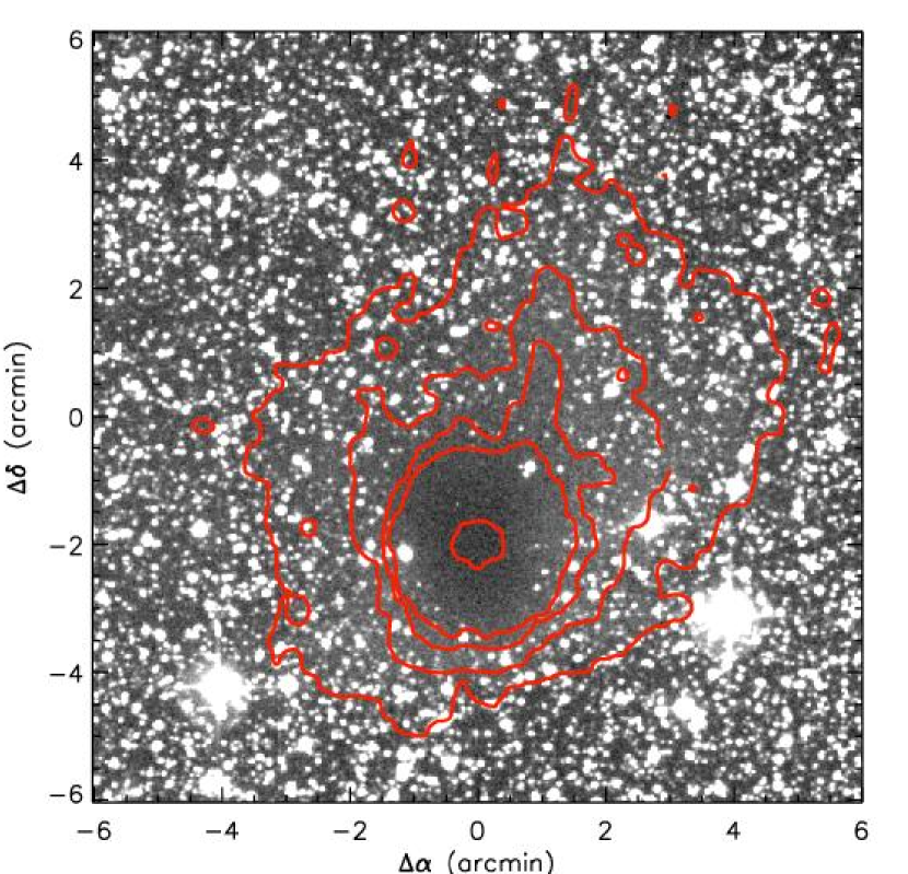
Figure 17.— Red Digital Sky Survey (DSS) image with 160 µm contours overlaid in red. The DSS image is displayed on a linear scale, centered on RA = $19^{h}37^{m}00.5^{s}$, Dec = $+07^{o}36\arcmin 10.0\arcsec$ ($2\arcmin$ north of the protostar). Contour levels are $\{0.2,0.5,0.8,1.1,10\}\times 1000$ mJy/arcsec².

Integrating over the SED plotted in Figure 2 for the point source component, we find a luminosity of $3.2$ L_☉ at an assumed distance of 250 pc, consistent with previous results. Adopting a distance of 150 pc, the luminosity becomes 1.2 L_☉. The larger beam data give a luminosity over a $180\arcsec$ region of 1.9 L_☉, peaking at 160 µm, for a distance of 150 pc. The difference, 0.7 L_☉, is consistent with heating by the interstellar radiation field: the interstellar radiation density is given by Cox & Mezger (1989) as 0.5 eV cm^-3. The interstellar flux incident on a sphere of radius $\sim\!0.07$ pc (corresponding to $90\arcsec$ at a distance of 150 pc) is, coincidentally, 0.8 L_☉. The opacity of B$335$ is such that we can expect most of this flux to be absorbed and reradiated in the far infrared, thus producing diffuse emission from the cloud at a level consistent with our observations (see Fig. 17).

Detailed modeling of the present data set is deferred to a subsequent work. However, to place B$335$ into context, we have compared its properties with those of the grid of models recently made available on the web by Robitaille et al. (2006) and Robitaille et al. (2007). These models for young protostars include disk and envelope components, scattered light, and outflow driven cavities. The SED is computed for a range of viewing angles, and the distance to the source can be varied as well.

We input into the SED modeler the stellar mass range of 0.3 to 0.5 $\hbox{M}_{\odot}$. The range of selected models is plausible and the general shape of the model SED’s match the observed photometry. We also fit the observed photometry (shown in Table 2) with a range of distances from 100 pc to 300 pc. The fitter prefers models with lower distances and high inclinations, which corroborates our distance estimate and agrees with the observed geometry of the source. The best-fit model has a $\chi^{2}=561$, a mass of 0.3 $\hbox{M}_{\odot}$, a distance of 100 pc, an inclination $\sim\!87\arcdeg$, and a disk outer radius of 145 AU, in good agreement with the Harvey et al. (2003a) measurement. If B$335$ is placed at the traditional distance of 250 pc, the calculated luminosity exceeds that expected from a $\sim\!0.5$ M_⊙ protostar and it is difficult to find a consistent solution without invoking asymmetric output of the far infrared flux. The set of 10 models with lowest $\chi^{2}$ values generally agree with this best-fit scenario, with stellar masses ranging from $\sim\!0.2$ to 0.7 $\hbox{M}_{\odot}$. Masses derrived from fitting SEDs to models are currently very uncertain; however, these masses fall in an interesting range and are only $\sim\!5$% of the total globule mass.

6. Conclusions

We report and analyze new Spitzer 3.6 to 160 µm data observations of B$335$  along with new ground based data in ¹²CO and ¹³CO.

1.) We revise the estimated distance from 250 pc to 150 pc. Our preferred distance is more compatible with the extinction models of Harvey et al. (2001) and with models of the embedded protostar (Robitaille et al., 2006, 2007).

2.) We discover an 8.0 µm shadow and derive a density profile for radii ranging from $\sim\!3,000$ to 7,500 AU. The shadow opacity at maximum is equivalent to $A_{V}$ = 100 or more.

3.) We detect a rotating structure in ¹²CO on scales of $\sim\!10000$ AU which we term a flattened molecular core. This structure is coaxial with the central circumstellar disk.

4.) It is very likely that the 8.0µm shadow and the flattened molecular core originate from the same structure.

5.) We measure the luminosity of the protostar to be 1.2 L_⊙ (at 150 pc),in good agreement with models for young stars of the expected mass ($\sim\!0.4$ $\hbox{M}_{\odot}$) and general characteristics of the object.

As the prototypical isolated, star-forming dark globule, there is a huge literature on Barnard 335. Nonetheless, our mid- and far-infrared data from Spitzer and CO observations from the HHT provide new insights regarding the configuration of the collapse of the globule and the properties of the protostar. We have found that the new observations are roughly consistent with recent models. Further comparisons with the full suite of observations have the potential to improve our understanding of isolated star formation significantly.

References

- Andrews & Williams (2007) Andrews, S. M., & Williams, J. P. 2007, ApJ, 659, 705
- Arreaga-García et al. (2007) Arreaga-García, G., Klapp, J., Sigalotti, L. D. G., & Gabbasov, R. 2007, ApJ, 666, 290
- Aumann et al. (1990) Aumann, H. H., Fowler, J. W., & Melnyk, M. 1990, AJ, 99, 1674
- Backus et al. (2005) Backus, C., Velusamy, T., Thompson, T., & Arballo, J. 2005, Astronomical Data Analysis Software and Systems XIV, 347, 61
- Bertin & Arnouts (1996) Bertin, E., & Arnouts, S. 1996, A&AS, 117, 393
- Blanco et al. (1970) Blanco, M., Demers, S., & Douglass, G. G. 1970, Publications of the U.S.Naval Observatory. Second Series, Washington: United States Government Printing Office (USGPO), 1970
- Bohlin et al. (1978) Bohlin, R. C., Savage, B. D., & Drake, J. F. 1978, ApJ, 224, 132
- Bok & Reilly (1947) Bok, B. J., & Reilly, E. F. 1947, ApJ, 105, 255
- Bok (1948) Bok, B. J. 1948, Centennial Symposia, 53
- Bouigue et al. (1961) Bouigue, R., Boulon, J., & Pedoussaut, A. 1961, Annales de l’Observatoire Astron. et Meteo. de Toulouse, 28, 33
- Cabrit & Bertout (1992) Cabrit, S., & Bertout, C. 1992, A&A, 261, 274
- Chandler et al. (1990) Chandler, C. J., Gear, W. K., Sandell, G., Hayashi, S., Duncan, W. D., Griffin, M. J., & Hazella, S. 1990, MNRAS, 243, 330
- Choi et al. (1995) Choi, M., Evans, N. J., II, Gregersen, E. M., & Wang, Y. 1995, ApJ, 448, 742
- Choi (2007) Choi, M. 2007, PASJ, 59, L41
- Clemens & Barvainis (1988) Clemens, D. P., & Barvainis, R. 1988, ApJS, 68, 257
- Cox & Mezger (1989) Cox, P., & Mezger, P. G. 1989, A&A Rev., 1, 49
- Davidson (1987) Davidson, J. A. 1987, ApJ, 315, 602
- de Luca et al. (1993) de Luca, M., Blanco, A., & Orofino, V. 1993, MNRAS, 262, 805
- Dickman (1978) Dickman, R. L. 1978, ApJS, 37, 407
- Draine (2003a) Draine, B. T. 2003a, ARA&A, 41, 241
- Draine (2003b) Draine, B. T. 2003b, ApJ, 598, 1017
- Evans et al. (2005) Evans, N. J., II, Lee, J.-E., Rawlings, J. M. C., & Choi, M. 2005, ApJ, 626, 919
- Fazio et al. (2004) Fazio, G. G., et al. 2004, ApJS, 154, 10
- Flaherty et al. (2007) Flaherty, K. M., Pipher, J. L., Megeath, S. T., Winston, E. M., Gutermuth, R. A., Muzerolle, J., Allen, L. E., & Fazio, G. G. 2007, ApJ, 663, 1069
- Frerking & Langer (1982) Frerking, M. A., & Langer, W. D. 1982, ApJ, 256, 523
- Gâlfalk & Olofsson (2007) Gâlfalk, M., & Olofsson, G. 2007, A&A, 475, 281
- Galván-Madrid et al. (2004) Galván-Madrid, R., Avila, R., & Rodríguez, L. F. 2004, Revista Mexicana de Astronomia y Astrofisica, 40, 31
- Gee et al. (1985) Gee, G., Griffin, M. J., Cunningham, T., Emerson, J. P., Ade, P. A. R., & Caroff, L. J. 1985, MNRAS, 215, 15P
- Gordon et al. (2005) Gordon, K. D., et al. 2005, PASP, 117, 503
- Harvey et al. (2001) Harvey, D. W. A., Wilner, D. J., Lada, C. J., Myers, P. C., Alves, J. F., & Chen, H. 2001, ApJ, 563, 903
- Harvey et al. (2003a) Harvey, D. W. A., Wilner, D. J., Myers, P. C., & Tafalla, M. 2003a, ApJ, 596, 383
- Harvey et al. (2003b) Harvey, D. W. A., Wilner, D. J., Myers, P. C., Tafalla, M., & Mardones, D. 2003b, ApJ, 583, 809
- Hirano et al. (1988) Hirano, N., Kameya, O., Nakayama, M., & Takakubo, K. 1988, ApJ, 327, L69
- Hodapp (1998) Hodapp, K.-W. 1998, ApJ, 500, L183
- Houck et al. (2004) Houck, J. R., et al. 2004, ApJS, 154, 18
- Huard et al. (1999) Huard, T. L., Sandell, G., & Weintraub, D. A. 1999, ApJ, 526, 833
- Indebetouw et al. (2005) Indebetouw, R., et al. 2005, ApJ, 619, 931
- Jørgensen et al. (2007) Jørgensen, J. K., et al. 2007, ApJ, 659, 479
- Keene et al. (1980) Keene, J., Hildebrand, R. H., Whitcomb, S. E., & Harper, D. A. 1980, ApJ, 240, L43
- Keene (1981) Keene, J. 1981, ApJ, 245, 115
- Keene et al. (1983) Keene, J., Davidson, J. A., Harper, D. A., Hildebrand, R. H., Jaffe, D. T., Loewenstein, R. F., Low, F. J., & Pernic, R. 1983, ApJ, 274, L43
- Krumholz et al. (2007) Krumholz, M. R., Klein, R. I., & McKee, C. F. 2007, ApJ, 665, 478
- Kutner & Ulich (1981) Kutner, M. L., & Ulich, B. L. 1981, ApJ, 250, 341
- Lallement et al. (2003) Lallement, R., Welsh, B. Y., Vergely, J. L., Crifo, F., & Sfeir, D. 2003, A&A, 411, 447
- Looney et al. (2007) Looney, L. W., Tobin, J. J., & Kwon, W. 2007, ApJ, 670, L131
- Lucy (1974) Lucy, L. B. 1974, AJ, 79, 745
- Makovoz & Marleau (2005) Makovoz, D., & Marleau, F. R. 2005, PASP, 117, 1113
- Martin & Barrett (1978) Martin, R. N., & Barrett, A. H. 1978, ApJS, 36, 1
- Mozurkewich et al. (1986) Mozurkewich, D., Schwartz, P. R., & Smith, H. A. 1986, ApJ, 311, 371
- Nelson & Langer (1997) Nelson, R. P., & Langer, W. D. 1997, ApJ, 482, 796
- Noriega-Crespo et al. (2004) Noriega-Crespo, A., et al. 2004, ApJS, 154, 352
- Ossenkopf & Henning (1994) Ossenkopf, V., & Henning, T. 1994, A&A, 291, 943
- Richardson (1972) Richardson, W. H. 1972, Journal of the Optical Society of America (1917-1983), 62, 55
- Rieke & Lebofsky (1985) Rieke, G. H., & Lebofsky, M. J. 1985, ApJ, 288, 618
- Rieke et al. (2004) Rieke, G. H., et al. 2004, ApJS, 154, 25
- Robitaille et al. (2006) Robitaille, T. P., Whitney, B. A., Indebetouw, R., Wood, K., & Denzmore, P. 2006, ApJS, 167, 256
- Robitaille et al. (2007) Robitaille, T. P., Whitney, B. A., Indebetouw, R., & Wood, K. 2007, ApJS, 169, 328
- Saito et al. (1999) Saito, M., Sunada, K., Kawabe, R., Kitamura, Y., & Hirano, N. 1999, ApJ, 518, 334
- Sault et al. (1995) Sault R.J., Teuben P.J., Wright M.C.H., 1995, in Astronomical Data Analysis Software and Systems IV, ed. R. Shaw, H.E. Payne, J.J.E. Hayes, ASP Conf. Ser., 77, 433-436
- Shirley et al. (2000) Shirley, Y. L., Evans, N. J., II, Rawlings, J. M. C., & Gregersen, E. M. 2000, ApJS, 131, 249
- Shirley et al. (2002) Shirley, Y. L., Evans, N. J., II, & Rawlings, J. M. C. 2002, ApJ, 575, 337
- Smith et al. (2007) Smith, J. D. T., et al. 2007, PASP, 119, 1133
- Stutz et al. (2007) Stutz, A. M., et al. 2007, ApJ, 665, 466
- Tomita et al. (1979) Tomita, Y., Saito, T., & Ohtani, H. 1979, PASJ, 31, 407
- van Dishoeck (2004) van Dishoeck, E. F. 2004, ARA&A, 42, 119
- Velusamy et al. (1995) Velusamy, T., Kuiper, T. B. H., & Langer, W. D. 1995, ApJ, 451, L75
- Velusamy et al. (2007) Velusamy, T., Langer, W. D., & Marsh, K. A. 2007, ApJ, 668, L159
- Velusamy et al. (2008) Velusamy, T., Marsh, K.A., Beichman, C.A., Backus, C.R., Thompson, T.J.2008, AJ (in press: to appear in July issue)
- Walker et al. (1990) Walker, C. K., Adams, F. C., & Lada, C. J. 1990, ApJ, 349, 515
- Whitehouse & Bate (2006) Whitehouse, S. C., & Bate, M. R. 2006, MNRAS, 367, 32
- Wilner et al. (2000) Wilner, D. J., Myers, P. C., Mardones, D., & Tafalla, M. 2000, ApJ, 544, L69
- Wu et al. (2007) Wu, J., Dunham, M. M., Evans, N. J., II, Bourke, T. L., & Young, C. H. 2007, AJ, 133, 1560
- Zhou et al. (1990) Zhou, S., Evans, N. J., II, Butner, H. M., Kutner, M. L., Leung, C. M., & Mundy, L. G. 1990, ApJ, 363, 168